HAL Id: hal-01109194
https://hal.inria.fr/hal-01109194
Submitted on 25 Jan 2015
HAL is a multi-disciplinary open access
archive for the deposit and dissemination of
sci-entific research documents, whether they are
pub-lished or not. The documents may come from
teaching and research institutions in France or
abroad, or from public or private research centers.
L’archive ouverte pluridisciplinaire HAL, est
destinée au dépôt et à la diffusion de documents
scientifiques de niveau recherche, publiés ou non,
émanant des établissements d’enseignement et de
recherche français ou étrangers, des laboratoires
publics ou privés.
Julio Araujo, Nicolas Nisse, Stéphane Pérennes
To cite this version:
Julio Araujo, Nicolas Nisse, Stéphane Pérennes. Weighted Coloring in Trees. SIAM Journal on
Discrete Mathematics, Society for Industrial and Applied Mathematics, 2014, 28 (4), pp.2029 - 2041.
�10.1137/140954167�. �hal-01109194�
JULIO ARAUJO†, NICOLAS NISSE‡, AND ST´EPHANE P´ERENNES‡
Abstract. A proper coloring of a graph is a partition of its vertex set into stable sets, where each part corresponds to a color. For a vertex-weighted graph, the weight of a color is the maximum weight of its vertices. The weight of a coloring is the sum of the weights of its colors. Guan and Zhu defined the weighted chromatic number of a vertex-weighted graph G as the smallest weight of a proper coloring of G (1997). If vertices of a graph have weight 1, its weighted chromatic number coincides with its chromatic number. Thus, the problem of computing the weighted chromatic number, a.k.a. Max Coloring Problem, is NP-hard in general graphs. It remains NP-hard in some graph classes as bipartite graphs. Approximation algorithms have been designed in several graph classes, in particular, there exists a PTAS for trees. Surprisingly, the time-complexity of computing this parameter in trees is still open.
The Exponential Time Hypothesis (ETH) states that 3-SAT cannot be solved in sub-exponen-tial time. We show that, assuming ETH, the best algorithm to compute the weighted chromatic number of n-node trees has time-complexity nΘ(log n). Our result mainly relies on proving that,
when computing an optimal proper weighted coloring of a graph G, it is hard to combine colorings of its connected components.
1. Introduction. Given a loop-less graph G = (V, E), a (proper) k-coloring of G is a surjective function c : V → {1, . . . , k} that assigns to each vertex v ∈ V a
color c(v) ∈ {1, . . . , k}, such that, for any {u, v} ∈ E, c(u) 6= c(v). Equivalently, a
k-coloring of G is a partition c = (S1, . . . , Sk) of V such that, for any 1 ≤ i ≤ k, Si is a non-empty independent set of vertices that have the same color i. One of the most studied problems in Graph Theory consists in minimizing the number of colors of a proper coloring of a graph. Namely, Graph Coloring aims at computing the
chromatic number of a graph G, denoted by χ(G), which is the minimum k for which
G has a k-coloring. This is one of the Karp’s NP-hard problems [8].
In [6], Guan and Zhu generalized Graph Coloring to vertex-weighted graphs. A (vertex) weighted graph (G, w) consists of a loop-less graph G = (V, E) and a weight function w : V → R+ over the vertices of G. Given a k-coloring c = (S1, . . . , Sk) of a weighted graph (G, w), the weight of color i (1 ≤ i ≤ k) is defined by w(i) = maxv∈Siw(v). The weight of coloring c is w(c) =
Pk
i=1w(i). The weighted chromatic
number of (G, w), denoted by χw(G), is the minimum weight of a proper coloring of (G, w). The Weighted Coloring Problem (also known as Max-coloring [15, 12, 13, 14, 11]) takes a weighted graph (G, w) and k ∈ R+ as inputs and asks whether χw(G) ≤ k [6].
Observe that if the weight of each of the vertices of a graph (G, w) is equal to one, then the weight of a coloring is the number of its colors and thus, χw(G) = χ(G). Therefore, Weighted Coloring generalizes Graph Coloring to weighted graphs, and, as a consequence, this problem is NP-hard in general graphs. Moreover, Weighted Coloringhas been shown NP-hard in bipartite graphs [3], where Graph Coloringis trivial. In the last years, the Weighted Coloring Problem has been addressed several times, however the complexity of this problem is surprisingly still unknown in the class of trees.
∗This work was partly funded by the ANR project GRATEL, and promoted by the
In-ria/FUNCAP project ALERTE and the Inria associate-team AlDyNet and CNPq–Brazil (contract PDE 202049/2012-4). An extended abstract of this work has been accepted in STACS 2014.
†ParGO Research Group, Departamento de Matem´atica, Universidade Federal do Cear´a,
Fort-aleza, Brazil
‡Inria and Univ. Nice Sophia Antipolis, CNRS, I3S, UMR 7271, Sophia Antipolis, France
Here, we show that, if 3-SAT cannot be solved in sub-exponential time (Expo-nential Time Hypothesis), then Weighted Coloring in trees is not in P.
Related work. Weighted Coloring has been shown to be NP-hard in the classes of split graphs, interval graphs, triangle-free planar graphs with bounded degree, and bipartite graphs [3, 14, 2, 5, 15]. On the other hand, the weighted chromatic number of cographs and of some subclasses of bipartite graphs can be found in polynomial-time [3, 2]. Constant-factor approximation algorithms have been designed for various graph classes such as interval graphs, perfect graphs, etc. [14, 11, 12, 13, 4]. In particular, it is known that Weighted Coloring can be approximated by a factor
8
7 in bipartite graphs and cannot be approximated by a factor 8
7− ǫ for any ǫ > 0 in this graph class unless P = N P [13].
Guan and Zhu showed that, given a fixed parameter r ∈ N, the minimum weight of a coloring using at most r colors can be computed in polynomial-time1 in the class of bounded treewidth graphs (a.k.a. partial k-trees) [6]. They left open the question of the time-complexity of the Weighted Coloring Problem in this class (partial k-trees) and, in particular, in trees. In [13], a sub-exponential algorithm and a polynomial-time approximation scheme to compute the weighted chromatic number of trees are presented. Later on, Escoffier et al. proposed a polynomial-time approx-imation scheme to compute the weighted chromatic number of bounded treewidth graphs [5]. Kavitha and Mestre recently presented polynomial-time algorithms for subclasses of trees [9]. They show that computing the weighted chromatic number can be done in linear time in the class of trees where nodes with degree at least three induce a stable set [9].
In the last years, many studies have been done on the Weighted Color-ing Problem, however the complexity of this problem was still unknown on trees. Weighted Coloringin trees has some intriguing properties. On the one hand, a reduction from another NP-hard problem was unlikely to exist due to the existence of a sub-exponential algorithm [13] (see also Section 2). Indeed, the problem cannot be NP-hard (under Karp reduction) unless problems in NP can be solved in time npolylog n - since the problem is solvable in nO(log n)(where n is the size of the input). On the other hand, all the classical methods to derive polynomial-time algorithms on trees failed [5, 9]. We provide here some explanation for these facts.
Our results. We show that, under the Exponential Time Hypothesis (ETH) (see Section 2), the best algorithm to compute the weighted chromatic number of trees has time-complexity nΘ(log n), where n is the number of vertices of the input tree. The existence of an algorithm that solves the Weighted Coloring Problem in time nΘ(log n) in bounded treewidth graphs follows easily from previous results. The difficulty is to prove that it is optimal under ETH. For this, we show that computing the weighted chromatic number of an n-node tree is as hard as deciding whether a 3-SAT formula with size log2n can be satisfied, where the size of a formula is its number of variables2. So, our reduction is rather technical, but we hope that it contains ideas that may be used in other contexts. Along the line of our reduction, one will discover another surprising aspect: the difficulty of the problem not only comes from the graph structure, but rather relies on the way weights are structured. This implies that choosing the right color for a node is hard. We indeed use non-binary constraint
1We emphasize that this algorithm is exponential in r
2Note that, in this paper, the number of clauses of the instances of SAT will always be
Figure 1. The unique optimal weighted coloring of (P4, w) uses strictly more than χ(P4) colors.
satisfaction formulae (i.e., constraint satisfaction formulae over positive integers) as main tool. Lastly, our reduction also proves that computing an optimal weighted coloring of a disconnected graph may be hard even if optimal colorings of each of its components can be done in polynomial-time.
Organization of the paper. The remainder of the paper is organized as follows. In Section 2, we formally state the main results of the paper: in Section 2.1, an nO(log n) -time algorithm is derived from previous works, and in Section 2.2 we prove our main result assuming a technical reduction (Proposition 2.2). The remaining part of the paper is devoted to the proof of Proposition 2.2. In Section 3, we give the main ideas of its proof. Finally, in Section 4, we prove a technical result (Proposition 3.3) which allows us to prove Proposition 2.2.
2. Preliminaries.
2.1. Sub-exponential algorithm. In this section, we show that there exists a sub-exponential algorithm to solve the Weighted Coloring Problem in the class of bounded treewidth graphs (including trees). This is an almost trivial consequence of previous works that mainly relies on the number of colors used by weighted colorings in these graphs.
There exist weighted graphs G for which any optimal weighted coloring uses strictly more than χ(G) colors: let us consider the 4-node path P4 with V (P4) = {a, b, c, d}, w(a) = w(d) = 4 and w(b) = w(c) = 1 (see Figure 1). Any color-ing of P4 with 2 = χ(P4) colors has weight 8, and the optimal weighted coloring {{a, d}, {b}, {c}} of (P4, w) has weight χw(P4) = 6 but uses 3 colors.
Luckily, the number of colors used by optimal weighted colorings can be bounded by O(log n) in the class of bounded treewidth graphs with n nodes. Indeed, Guan and Zhu studied the number of colors used by an optimal weighted coloring [6]. More precisely, they proved that the maximum number of colors of an optimal weighted coloring of a weighted graph (G, w) is its first-fit chromatic number χF F(G) (a.k.a.,
Grundy number) [6]. This is tight since, for any graph G, there exists a weight function
w such that an optimal weighted coloring of (G, w) uses χF F(G) colors. On the other hand, for any n-node graph G with tree-width at most k, χF F(G) = O(k log n) [10]. In particular, this implies that, for any n-node tree, there is an optimal weighted coloring using O(log n) colors. Finally, in the class of bounded treewidth graphs and when the number r ∈ N of colors is fixed, there is an algorithm (using dynamic programming on the tree-decomposition) that computes the minimum weight of a coloring using at most r colors in time polynomial in O(nr) where n is the number of vertices of the input graph [6].
By combining these results, the following proposition is straightforward:
Proposition 2.1. There exists an algorithm that solves the Weighted
Col-oring Problem in time nO(log n) in the class of bounded treewidth graphs (including trees), where n is the number of vertices of the input graph.
2.2. Main Result. We now formalize our main result. Recall that an instance of the 3-SAT Problem is any Boolean formula Φ(v1, . . . , vη) over the variables v1, . . . , vη
in the conjunctive normal form (CNF) where each clause involves at most three vari-ables. The size of Φ is its number of variables, denoted by η. The 3-SAT Problem asks whether there exists a truth assignment to the variables of Φ such that Φ(v1, . . . , vη) is true. It is well known that the 3-SAT Problem is NP-complete [1]. A fundamental question is to know whether it can be solved in sub-exponential time. Note that, otherwise, P 6= NP .
Conjecture 1. Exponential Time Hypothesis (ETH)[7].
3-SAT cannot be solved in time 2o(η)where η is the size of the instance. The main part of this paper is devoted to proving the following result.
Proposition 2.2. For any Boolean formula Φ of size η, there exist a weighted tree (T, w) with n = 2O(√η) vertices and M ∈ R such that Φ is satisfiable if and only
if χw(T ) ≤ M. Moreover, (T, w) and M are computable in time polynomial in n. Proposition 2.2 allows us to prove that there is no polynomial-time algorithm to solve the Weighted Coloring Problem in trees, unless ETH fails.
Theorem 2.3. If ETH is true, then the best algorithm to compute the weighted chromatic number of an n-node tree T has time-complexity nΘ(log n).
Proof. The existence of such an algorithm directly follows from Proposition 2.1.
For purpose of contradiction, let us assume that there exists an algorithm A that solves the Weighted Coloring Problem in time no(log n)in the class of trees, where n is the number of vertices of the input tree. Let Φ be any Boolean formula of size η. By Proposition 2.2, there exists a weighted tree (T, w) with n = 2O(√η) = 2o(η) vertices and M ∈ R such that Φ is satisfiable if and only if χw(T ) ≤ M. Consider the following algorithm to solve 3-SAT. For any Boolean formula Φ of size η, first compute (T, w) and M in time 2o(η), then use Algorithm A to compute χw(T ) in time no(log n) = 2o(η). By definition, Φ is satisfiable if and only if χw(T ) ≤ M. Therefore, the above algorithm solves the 3-SAT Problem in time 2o(η)where η is the size of the instance, contradicting ETH.
Note that our result is actually stronger since we prove that if the Weighted Coloring Problem can be solved in time no(logn) in n-node trees then 3-SAT is solvable in time 2O(√n).
The remaining part of the paper is devoted to the proof of Proposition 2.2. 3. From boolean variables to integral variables. Proposition 2.2 establishes a link between the Weighted Coloring Problem and 3-SAT. Informally, to evaluate the time-complexity of the Weighted Coloring Problem, the ideal way would be to reduce any 3-SAT formula Φ to a weighted tree (T, w) such that (1) there is a correspondence between truth assignments of the variables of Φ and the optimal colorings of T , and (2) Φ is satisfiable if and only if χw(T ) is at most some pre-defined value M (depending on Φ). To do such a reduction, we would like to proceed as follows: given a boolean formula Φ of size η, we build a weighted tree T such that any truth assignment of Φ for which Φ is satisfied, we have a coloring of T of bounded weight, where the weight of a color reflects the truth assignment of a variable. Hence, the desired weighted tree T must be such that any optimal coloring of T uses η colors. However, proceeding that way, since the number of colors in an optimal weighted coloring of an n-node tree is at most O(log n), T must have at least n = 2η nodes. Hence, a polynomial-time algorithm to solve the Weighted Coloring Problem in T would only lead to an exponential-time algorithm for deciding whether Φ is satisfiable.
3.1. From 3-SAT to INT-SAT. To bypass the above problem, we will use an auxiliary formula. Intuitively, given a 3-SAT formula with η boolean variables, we will translate it into another logical formula with √η integral variables. Using this new
formula, we build a tree with 2√η nodes, where the weights of the colors in coloring of bounded weight will correspond to the integral values of the variables. Note that our method is close to the Split and List method of [16]. More formally,
Definition 3.1. Given a set of n × m boolean variables (yi
j)0≤i<n,0≤j<m, an integral assignment of these variables is a truth assignment such that, for any 0 ≤ i < n, exactly one variable yi
j, 0 ≤ j < m, receives value 1.
A boolean formula Φ with n × m boolean variables (yi
j)i<n,j<m is integrally sat-isfiable w.r.t. (yi
j)0≤i<n,0≤j<m if there is an integral assignment of its variables that
satisfies Φ.
The INT-SAT Problem takes a formula Φ with variables (yi
j)0≤i<n,0≤j<mas input
and asks whether Φ is integrally satisfiable w.r.t. (yi
j)0≤i<n,0≤j<m.
In what follows, we widely use the fact that there is a one-to-one mapping between any integral assignment of a set of n × m boolean variables (yi
j)i<n,j<m and the set of n-tuples (x0, . . . , xn−1) of integers in {0, . . . , m − 1}. Indeed, for any 0 ≤ i < n, xi = j where 0 ≤ j < m is the unique index such that yi
j = 1.
We now show that 3-SAT can be sub-exponentially reduced to INT-SAT. This is an important ingredient of the proof of Proposition 2.2. We also think this result has its own interest and could be used in other contexts.
Theorem 3.2. For any instance Φ of 3-SAT with size η, there is a Boolean for-mula Φint of size n = 2O(
√η)
, with variables (yi
j)0≤i<√η,0≤j<2√η, s.t. Φ is satisfiable
if and only if Φint is integrally satisfiable w.r.t. (yij)i,j. Φint can be computed in time O(n) and it is a CNF formula where all variables appear positively.
Proof. Let Φ(u0, . . . , uη−1) be an instance of 3-SAT of size η = N2 (if η 6= N2, we can add dummy variables). For any two integers a < N and b < 2N, let bit(a, b) correspond to the a-th bit of the binary representation of b.
Let Φint be the formula obtained from Φ by replacing each literal uiN+j, 0 ≤ i < N and 0 ≤ j < N, byW{ℓ|bit(j,ℓ)=1, 0≤ℓ<2N}vℓi. Then, each literal ¯uiN+j, 0 ≤ i < N
and 0 ≤ j < N is replaced by W{ℓ|bit(j,ℓ)=0, 0≤ℓ<2N}vℓi. Hence, Φint has N · 2N
variables
(v00, . . . , v02N−1, v01, . . . , v21N−1, . . . , v0N−1, . . . , vN2N−1−1)
and poly(N ) clauses of size O(2N). Because Φ is in CNF, it is also the case for Φint. Moreover, all variables appear positively in Φint.
It remains to show that Φintis integrally satisfiable if and only if Φ is satisfiable. First, let us assume that Φ is satisfiable. Let u0, . . . , uη−1be a valid assignment of its variables and, for any 0 ≤ i < N, let xi be the integer with (uN i, . . . , uN(i+1)−1) as binary representation. Note that xi∈ {0, · · · , 2N−1}. Finally, for any 0 ≤ i < N and 0 ≤ j < 2N, let us define vi
j = 1 if xi = j and vji = 0 otherwise. By definition of Φint, (vi
j)0≤i<N, 0≤j<2N is a valid assignment and Φint is therefore integrally satisfiable.
Conversely, let us assume that Φint is integrally satisfiable and let (x0, . . . , xN−1) be N integers representing a valid assignment for it. Let u0, . . . , uη−1 be defined such that, for any 0 ≤ i < N, (uN i, . . . , uN(i+1)−1) is the binary representation of xi. Then, u0, . . . , uη−1 is a satisfying assignment for Φ which is satisfiable.
3.2. Proof of Proposition 2.2. Theorem 3.2 allows us to reduce any 3-SAT instance Φ of size η into an INT-SAT instance Φint with size 2O(√η). For simplicity of presentation, we assume that √η is an integer. The key point is that this reduction allows us to turn the choice of η boolean variables into the choice of √η integers in {0, . . . , 2√η− 1}. Then, in further sections, we build a tree T with 2O(√η) vertices
from the formula Φint, such that there is a one to one mapping between any optimal weighted coloring of T and the √η-tuples of integers in {0, . . . , 2√η− 1}. Finally, our reduction ensures that the value of χw(T ) depends on the integral satisfiability of Φint and therefore, on the satisfiability of Φ. More formally, the next section is devoted to proving the following result:
Proposition 3.3. For any CNF Boolean formula Φint of size η = n2n where all
variables (yi
j)i,j appear positively, there exist a weighted tree (T (Φint), w(Φint)) with
size polynomial in η and M ∈ R s.t. Φint is integrally satisfiable w.r.t. (yji)i,j if and
only if χw(T (Φint)) ≤ M. The pair (T (Φint), w(Φint)) and M are computable in time
polynomial in η.
The proof of Proposition 2.2 is straightforward from Theorem 3.2 and Proposition 3.3. 4. Proof of Proposition 3.3. This section is devoted to the proof of Proposi-tion 3.3.
Let us introduce some notations. Let n ∈ N and let m = 2n. Let Φint be a Boolean formula with n × m variables {yij | 0 ≤ i < n, 0 ≤ j < m} and L clauses, where L is polynomial in n. We assume that Φint is a CNF formula and that each variable appears positively. Moreover, we may assume that each variable appears at least once. That is, Φint =Vℓ≤LQℓ and, for any 1 ≤ ℓ ≤ L, Qℓis the disjunction of pℓ≥ 1 positive variables.
Let ǫ > 0 such that nmǫ = o( 1
24n) and let M = 4n+2X i=0 1 2i + n(m − 1)ǫ < 2.
Let wji = 1/2i+ jǫ, for any 0 ≤ i ≤ 4n + 3 and 0 ≤ j ≤ m. Let W = {wj i | 0 ≤ i ≤ 4n + 3, 0 ≤ j ≤ m} denote a set of weights. Note that the length of the encoding of these weights is polynomially bounded. For any 0 ≤ k ≤ 3, let Wk = w0
4n+k = 1/24n+k. Finally, for any rooted tree T , let r(T ) denote its root. A rooted tree S is a (proper) subtree of a rooted tree T if there is an edge e of T such that S is the connected component of T \ {e} that does not contain r(T ). We now define various subtrees required to build (T (Φint), w).
4.1. Binomial trees. We first define a particular family of binomial trees Bi, 0 ≤ i ≤ 4n + 2. They will be used in the construction of T (Φint). Their role is to force the color of most of the nodes in any coloring c of T (Φint) with w(c) ≤ M. Note that, the notion of binomial trees has also been used in [2].
Definition 4.1. For any 0 ≤ i ≤ 4n + 2, let Bi be the weighted rooted tree
defined recursively as follows (see Figure 2).
• if i = 0, then B0 has a unique node with weight w0 0; • otherwise, Bi has a root of weight w0
i whose children are the roots of copies
of B0, B1, . . . , Bi−1.
Note that Bi has 2i nodes and that it just contains nodes of weight w0 j, for 0 ≤ j ≤ i ≤ 4n + 2. We will use these binomial trees with two main goals in our reduction:
• enforce the number of used colors and the weights of these colors (up to an additive constant cǫ) in any optimal weighted coloring of the tree we build from the 3-SAT formula;
• forbid the color i to appear in any vertex that is adjacent to a root of a binomial tree Bi.
Figure 2. The construction of the binomial tree Bi.
We get these properties according to the following lemmas:
Lemma 4.2. Let 0 ≤ i ≤ 4n + 2. Let (T, w) be a weighted tree having Bi as
subtree. If there exists a coloring c of (T, w) with w(c) ≤ M, then, for any 0 ≤ k ≤ i: 1. all vertices of Bi with weight in wk0 receive the same color Sk of c; and
2. there exists a unique color class Sk in c of weight in {wkj | 0 ≤ j ≤ m}.
Proof. The proof is by induction on the index i. In case i = 0, we prove both
statements of the lemma at once by observing that any two vertices of (T, w) of weight in {wj0′ | 0 ≤ j′ ≤ m} must belong to the same color class S0, otherwise we would conclude that w(c) ≥ 2, that would be a contradiction to the fact that w(c) ≤ M < 2. Now, let 0 ≤ k ≤ i, observe that the set of nodes of Bi with weight in w0 k is an independent set that dominates the nodes of Bi with smaller weights (i.e., in {w0
k′ | k < k′ ≤ i}).
By induction hypothesis, for any 0 ≤ k < i, the set of nodes of Bi with weight in w0
k receive the same color Sk of c and this color class is the unique with weight in {wkj | 0 ≤ j ≤ m}. Then, for any 0 ≤ k < i, the root of Bi cannot be colored Sk, since it has a neighbor with weight w0
k. Let Sibe the color of the root of Biin c. We proved that the color Si cannot contain nodes with weight greater than wim−1 and that c cannot have another color S′
i 6= Si with weight in {w j
i | 0 ≤ j ≤ m}, because, otherwise the weight of c would be at least 21i +
Pi
k=021k = 2 > M in both cases.
Corollary 4.3. Let (T, w) be a weighted tree having B4n+2 as subtree. Let c be
any coloring of (T, w) s.t. w(c) ≤ M. Then, c = (S0, . . . , Sk) with k ≥ 4n + 2 and,
for any 0 ≤ i ≤ 4n + 2, Si is the unique color with weight in {wji | 0 ≤ j ≤ m}. The trees we consider below will always satisfy the requirements of Corollary 4.3. Therefore, we are able to identify a color by its weight. In other words, in what follows, for any coloring c = (S0, . . . , Sk) of weight at most M and for any i ≤ 4n + 2, Si will be the unique color such that w(Si) ∈ {wji | 0 ≤ j ≤ m}.
Recall that we defined, for any 0 ≤ k ≤ 3, Wk = w0
4n+k = 1/24n+k. By a slight abuse of notation, for any 0 ≤ k ≤ 3, we denote Wk = S4n+kas the unique color with weight Wk.
4.2. Auxiliary trees and Variable-trees. This section is mainly devoted to the construction of subtrees that will represent the boolean variables. First, the family of auxiliary trees Aji, 0 ≤ i < 4n, 0 ≤ j ≤ m, will be used to introduce some choice
when coloring T (Φint).
Definition 4.4. For any 0 ≤ i < 4n, 0 ≤ j ≤ m, let Aji be the weighted rooted
tree defined as follows (see Figure 3). Note that Aji consists of 24n nodes.
1. Let u be its root with weight w(u) = W0, and connect it to a node v (its subroot) with weight w(v) = wji;
2. v is made adjacent to the root of a copy of Bℓ, for any 0 ≤ ℓ < i − 1;
3. u is made adjacent to the root of a copy of Bℓ, for any 0 ≤ ℓ < 4n, ℓ 6= i − 1.
Figure 3. Auxiliary tree Aji.
Figure 4. The variable tree T (yji).
Lemma 4.5. Let 0 ≤ i < 4n and 0 ≤ j ≤ m. Let (T, w) be any weighted tree
having B4n+2 and Aji as subtrees. Let u and v be the root and the sub-root of Aji,
respectively. For any coloring c of (T, w) with weight w(c) ≤ M, then it holds:
• either v is colored Si−1 and u must be colored with the color W0;
• or v is colored Si (therefore, w(Si) ≥ wji) and u is colored either with Si−1
or with W0.
Proof. Recall that, by Corollary 4.3, we can identify the colors of c and their
weights. By Lemma 4.2, the root of each subtree Bk, 0 ≤ k < 4n, must be colored with Sk and then the sub-root v can be colored only with color Si−1 or Si. Note that, if v is colored with color Sp for some p > i, then w(Sp) ≥ wji, contradicting Corollary 4.3. In the first case, u is adjacent to a node with color Sk, for any k < 4n. Therefore, u must be colored with color S4n= W0.
Otherwise, u is adjacent to a node with color Sk, for any k < 4n but k = i − 1. Moreover, u cannot be colored with Sk for k > 4n since otherwise, w(c) > M (Sk would have weight strictly more than wk). Hence, u can only be colored with Si−1 or W0.
Intuitively, the previous lemma states that, either we “pay” jǫ in the weight of color Si, or u must be colored with the color W0. We now define the variable-trees T (yij) using the auxiliary trees.
Definition 4.6. For any 0 ≤ i < n, 0 ≤ j < m, let T (yij) be the weighted rooted
tree, representing the variable yij, defined as follows (see Figure 4):
• let u be its root with weight w(u) = W1 and connected to the root of a copy of Bℓ, for any 0 ≤ ℓ < 4n;
• take one copy of Aj4i+1, A j+1 4i+1, A m−j 4i+3 and A m−1−j 4i+3 and:
– connect r(Aj4i+1) to r(Am−j4i+3), and r(Aj+14i+1) to r(Am−1−j4i+3 ); – connect u with r(Aj4i+1) and r(Am−j−14i+3 ).
Note that T (yji) consists of O(24n) nodes (i.e. polynomial in nm).
Intuitively, setting the color of the root of variable-tree T (yji) to W0 or W1 will correspond to setting the corresponding variable yijto true or false respectively. More-over, next lemma shows that, for a fixed i, the weights of the classes S4i+3and S4i+1 impose that at most one variable yij, 0 ≤ j < m, is set to true.
Lemma 4.7. Let (T, w) be any weighted tree having B4n+2 as subtree and
con-taining T (yij) as subtree, for all 0 ≤ i < n and 0 ≤ j < m. Let c be a coloring of T
with weight w(c) ≤ M.
Then, there are (j0, . . . , jn−1) ∈ {0, . . . , m − 1}n such that each root u of each
subtree T (yij), for any 0 ≤ i < n and 0 ≤ j < m, satisfies: • if j 6= ji, then the color of u in c must be W1;
• otherwise, no neighbors of u in T (yji) is colored with W0 and u is colored
either W0 or W1.
Proof. Since T contains B4n+2, by Corollary 4.3, a coloring c = (S0, . . . , Sk) of weight w(c) ≤ M is such that k ≥ 4n + 2, and, for any 0 ≤ i ≤ 4n + 2, Siis the unique color such that w(Si) ∈ {wji | 0 ≤ j ≤ m}. In particular, w(c) ≥
P4n+2 i=0 1/2i = M − n(m − 1)ǫ.
For any 0 ≤ i < n, let 0 ≤ ji≤ m be such that w(S4i+1) = wji
4i+1.
First, let us assume that ji < m. In particular, this means that every sub-root of a subtree Ar
4i+1, for each ji < r ≤ m, is colored S4i (recall that its color is either S4i or S4i+1, by Lemma 4.5). Consequently, any root of a subtree Ar
4i+1, for each ji < r ≤ m, must be colored W0. Therefore, by the construction of the variable-trees, any root of a subtree Am−r4i+3, for each ji < r ≤ m, cannot be colored W0 because it is adjacent to a root of a subtree Ar
4i+1. Thus, by Lemma 4.5, it must be colored S4i+2 and the color of each sub-root of Am4i+3−r must be S4i+3. Consequently, w(S4i+3) ≥ wm−(ji+1)
4i+3 . Hence, for any 0 ≤ i < n, if ji < m, we conclude that w(S4i+3) + w(S4i+1) ≥ wji
4i+1+ wm−(j
i+1)
4i+3 = (m − 1)ǫ + 1/24i+1+ 1/24i+3.
On the other hand, if ji = m, it follows directly that w(S4i+3) + w(S4i+1) ≥ mǫ + 1/24i+1+ 1/24i+3.
Since w(c) ≤ M, it implies that, for any 0 ≤ i < n, ji < m and w(S4i+3) = wm−ji−1
4i+3 and, for any 0 ≤ 2k < 4n, w(S2k) = w02k. Consequently, since w(S4i+3) = wm−ji−1
4i+3 , by a similar argument, the roots of all subtrees Am−j4i+3, for each 0 ≤ j ≤ ji, must be colored W0 and, then, the roots of all subtrees Aj4i+1, for each 0 ≤ j ≤ ji, must be colored S4i.
Let 0 ≤ i < n and 0 ≤ j < m. Consider a subtree T (yij) of T . If j 6= ji, then (exactly) one of the roots of Aj4i+1 and Am4i+3−1−j must be colored W0. In that case, the color of the root u of T (yij) must be W1. Indeed, u is adjacent to the root of Bk, 0 ≤ k < 4n, and therefore it cannot be colored Sk. Moreover, if u is colored W2, then we have a contradiction as w(c) > M , because w(u) = W1. On the other hand, if j = ji, the root of Aj4i+1 is colored with S4i and the root of Am−1−j4i+3 is colored with S4i+2. In particular, none of the roots of Aj4i+1 and Am−1−j4i+3 are colored with W0. Therefore, u is colored either W0 or W1 (u cannot have color Sk for k > 4n + 1 since otherwise w(c) > M ).
4.3. Clause-trees and definition of T (Φint). We define the subtrees repre-senting the clauses and combine them to get T (Φint).
Definition 4.8. Let 1 ≤ ℓ ≤ L and let Qℓ = ∨1≤k≤pℓuk be any clause of Φint
1 ≤ k ≤ pℓ, let T (Qk
ℓ) be the rooted weighted tree defined recursively as follows:
1. T (Q1
ℓ) = T (u1);
2. for any k > 1, start with one copy of T (Qk−1ℓ ) with root a and one copy
of T (uk) with root b. Let g, d be two nodes with weight W1 and e, f be
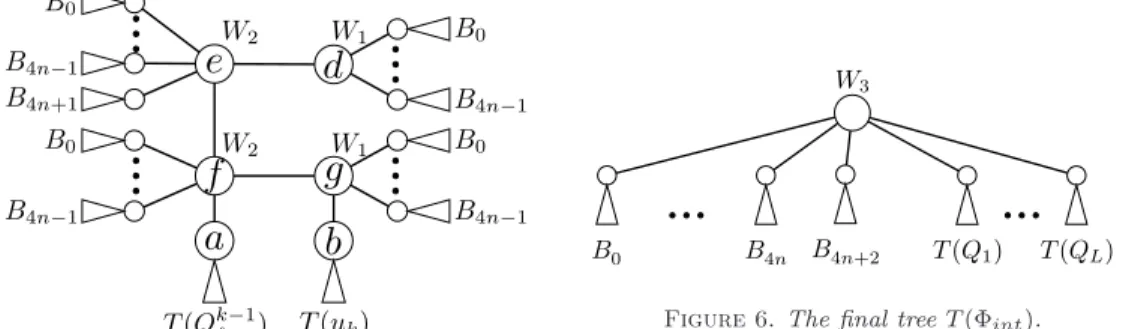
two nodes with weight W2. For each node v ∈ {g, d, e, f}, and for any 0 ≤ i < 4n, add one copy of Bi and make its root adjacent to v. Add one copy of B4n+1 and make its root adjacent to e. Finally, we add the edges {{a, f}, {b, g}, {g, f}, {d, e}, {e, f}} and d is chosen as the root.
Let us note T (Qℓ) = T (Qpℓ
ℓ ) the clause-tree corresponding to Qℓand that consists of O(pℓ24n) nodes (i.e. polynomial in nm). T (Qk
ℓ) is depicted in Figure 5.
Figure 5. The clause tree T (Qk ℓ).
Figure 6. The final tree T (Φint).
The next lemma describes how a coloring of a clause-tree T (Qk
ℓ) expresses the fact that the corresponding clause ∨1≤h≤kuh is satisfied or not. Informally, the color of the root of T (Qk
ℓ) must be W1 if the clause is not satisfied, i.e., if ∨1≤h<kuhis not satisfied (in which case, the root a of T (Qk−1ℓ ) is colored W1) and if uk is assigned to false (in which case, the root b of T (uk) is colored W1). Otherwise, it will be possible to color the root of T (Qk
ℓ) with W0.
Lemma 4.9. Let (T, w) be any weighted tree having B4n+2 as subtree and
con-taining T (Qk
ℓ) as a subtree (1 ≤ ℓ ≤ L, 1 ≤ k ≤ pℓ) where Qkℓ = ∨1≤h≤kuh is the
prefix of a clause of Φint. Let c be any coloring of T with weight w(c) ≤ M. The
color of d is either W0 or W1. Moreover, if a and b are colored W1, then the color of
the root d of T (Qk
ℓ) must be W1;
Proof. We prove it by induction on the number of variables k of Qk
ℓ. Observe that in case k = 1, then T (Qk
ℓ) is a variable-tree and the lemma trivially holds. Indeed, vertices a, g, d, e, f do not exist and the root is b, thus the first statement is trivially satisfied, and, by Lemma 4.7, the color of its root must be either W0 or W1.
Now, consider that a and b are roots of a clause-tree on k − 1 variables T (Qkℓ−1) and of a variable-tree, respectively. By Lemma 4.7 and by the inductive hypothesis, the colors of a and b are either W0 or W1.
In case c(a) = c(b) = W1, by the hypothesis w(c) ≤ M, by Lemma 4.2 and Corollary 4.3, we conclude that g is colored W0, f is colored W2, e is colored W0 (note that it is possible since no subtree B4n is adjacent to e) and d is forced to be colored W1.
Finally, by the construction of T (Qk
ℓ), by Lemma 4.2 and Corollary 4.3, the root d may be colored either W0 or W1, since w(c) ≤ M.
Definition 4.10. Let T (Φint) be the weighted rooted tree obtained as follows
(see Figure 6). Let r be the root with weight W3. For any 1 ≤ ℓ ≤ L, the root of one
adjacent to the root of one copy of Bi.
Lemma 4.11. T (Φint) has size polynomial in m = 2n.
Proof. Observe that each clause-tree T (Qℓ) has size O(pℓ24n) (see Definition 4.8), where pℓis polynomial in m (since pℓis at most the number nm of variables). More-over, the number L of clauses is polynomial in m by the definition of Φint.
Lemma 4.12. If Φint is integrally satisfiable, then χw(T (Φint)) ≤ M.
Proof. Let (yji)0≤i<n,0≤j<m be a valid integral assignment for Φint. For any 0 ≤ i < n, let ji be the (unique) index such that yji
i is true. We construct a coloring c of (T (Φint), w) such that w(c) ≤ M. By Lemma 4.2, in any coloring c of T (Φint) such that w(c) ≤ M, the colors of all nodes of the binomial subtrees of T (Φint) are forced. Consequently, we only need to decide the colors of the following nodes: the roots and sub-roots of any copy of Aji, the roots of the trees T (yji), and the nodes connecting the variables-trees into clause-trees (the nodes a, b, g, d, e, f in Figure 5), for any 0 ≤ i < n and 0 ≤ j < m.
We first set the weight of color Si for any 0 ≤ i < 4n. In particular, for any 0 ≤ i < n, the color S4i+1 must have weight wj4i+1i . As we observed in the proof of Lemma 4.7, this choice fixes the colors of all roots and sub-roots of all the Aji trees, i.e. all the nodes in the variable trees, except to the roots of the variable-trees T (yji
i ), by Lemma 4.7.
More precisely, for any 0 ≤ i < n and 0 ≤ j < m, let us consider a subtree T (yji). Let j′ ∈ {j, j + 1}. The sub-root of Aj′
4i+1 receives color S4i+1 if j′ ≤ ji and receives color S4i otherwise. The root of Aj4i+1′ receives color S4i if j′ ≤ ji and receives color W0otherwise. The sub-root of Am−j4i+3′ receives color S4i+3if j′ > ji and receives color S4i+2 otherwise. The root of Am4i+3−j′ receives color S4i+2 if j′ > ji and receives color W0 otherwise. Finally, if j 6= ji, the root of T (yji) is colored W1. On the other hand, if j = ji, none of the neighbors of the root of T (yij) is colored W0, therefore, we can color it either W0 or W1.
Now, let Qℓ =W1≤k≤pℓuk be any clause of Φint. We show that we can extend the previous coloring such that the root of the clause-tree T (Qℓ) is colored W0 and the weight of the coloring is ≤ M. This is by induction on pℓ. Indeed, if pℓ= 1, then Qℓ consists of a unique variable and this variable must be assigned to true (since the formula is true). Hence, Qℓ = yji
i for some 0 ≤ i < n. That is T (Qℓ) is a subtree T (yji
i ). Hence, we can color the root of it with W0.
Now, assume that the result is correct for any clause of length p ≥ 1 and let pℓ= p + 1. Thus, Qℓ= up+1∨(W1≤k≤puk). Recall that T (Qℓ) is built from a variable subtree T (up+1) and a clause-subtree T (Qpℓ). There are two cases to consider: either our assignment satisfies W1≤k≤puk or not. In the first case, the root of the clause-tree T (Qpℓ) (node a in Figure 5) is colored W0 by induction. Moreover, by above paragraphs, the root of T (up+1) (node b in Figure 5) can be colored W1. It is then easy to extend this coloring such that the root of T (Qℓ) is colored W0: in Figure 5, node f is colored W1, node e is colored W2 and nodes g and d are colored W0. If our assignment does not satisfyW1≤k≤puk, then it must satisfy up+1. That is, up+1= yji
i for some 0 ≤ i < n. By a similar induction, we prove that the root of T (Qpℓ) can be colored W1. Moreover, by above paragraphs, the root of T (up+1) = T (yji
i ) can be colored W0. This coloring can be extended such that the root of T (Qℓ) is colored W0: in Figure 5, node g is colored W1, node e is colored W2and nodes f and d are colored W0.
Thus, we color the roots of all the clause-trees with color W0 and the root of T (Φint) with the color W1.
Hence, the weight of this coloring c is w(c) =P4n+2i=0 21i + n(m − 1)ǫ = M.
Lemma 4.13. If Φint is not integrally satisfiable, then χw(T (Φint)) > M .
Proof. Φint is not integrally satisfiable. For purpose of contradiction, let c be a coloring of T (Φint) with weight at most M . By Lemma 4.7, there are integers (j0, . . . , jn−1) such that the color of the root of any subtree T (yij) is forced to be W1, if j 6= ji. Let Y = (yji)i<n,j<m be the corresponding integral assignment. In other words, for any variable yij (0 ≤ i < n, 0 ≤ j < m), yji = 0 if j 6= ji. Since Φint is not integrally satisfiable, there is a clause Q that is not satisfied by this assignment. Let us consider the clause-subtree T (Q). It has been built from variable-trees corresponding to the variables constituting the clause Q. Because all these variables are assigned to false, the roots of these variable-trees are all colored with W1, by Lemma 4.7.
By induction on the length of Q and by Lemma 4.9, the color of the root of T (Qℓ) must be W1. Thus, the root of T (Φint) can only be colored W3. Consequently, the coloring c has weight w(c) ≥P4n+3i=0 21i + n(m − 1)ǫ > M, a contradiction.
Proposition 3.3 follows directly from Lemmas 4.11, 4.12 and 4.13.
REFERENCES
[1] Stephen A. Cook, The complexity of theorem-proving procedures, in Proceedings of the 3rd Annual ACM Symp. on Theory of Computing (STOC), 1971, pp. 151–158.
[2] Dominique de Werra, Marc Demange, Bruno Escoffier, J´erˆome Monnot, and Vange-lis Th. Paschos, Weighted coloring on planar, bipartite and split graphs: Complexity and approximation, Discrete Applied Mathematics, 157 (2009), pp. 819–832.
[3] Marc Demange, Dominique de Werra, J´erˆome Monnot, and Vangelis Th. Paschos, Weighted node coloring: When stable sets are expensive, in 28th Int. Work. on Graph-Theoretic Concepts in Comp. Sc. (WG), vol. 2573 of LNCS, Springer, 2002, pp. 114–125. [4] Leah Epstein and Asaf Levin, On the max coloring problem, Theor. Comput. Sci., 462 (2012),
pp. 23–38.
[5] Bruno Escoffier, J´erˆome Monnot, and Vangelis Th. Paschos, Weighted coloring: further complexity and approximability results, Inf. Process. Lett., 97 (2006), pp. 98–103. [6] D. J. Guan and Xuding Zhu, A coloring problem for weighted graphs, Inf. Process. Lett., 61
(1997), pp. 77–81.
[7] Russell Impagliazzo and Ramamohan Paturi, On the complexity of k-SAT, J. Comput. Syst. Sci., 62 (2001), pp. 367–375.
[8] Richard M. Karp, Reducibility among combinatorial problems, in Proceedings of a sympo-sium on the Complexity of Computer Computations, The IBM Research Symposia Series, Plenum Press, New York, 1972, pp. 85–103.
[9] Telikepalli Kavitha and Juli´an Mestre, Max-coloring paths: tight bounds and extensions, J. Comb. Optim., 24 (2012), pp. 1–14.
[10] C. Linhares Sales and B. Reed, Weighted coloring on graphs with bounded tree width, in Annals of 19th International Symposium on Mathematical Programming, 2006.
[11] Sriram V. Pemmaraju, Sriram Penumatcha, and Rajiv Raman, Approximating interval coloring and max-coloring in chordal graphs, in Proc. 3rd Int. Workshop on Experimental and Efficient Algorithms (WEA), vol. 3059 of LNCS, Springer, 2004, pp. 399–416. [12] , Approximating interval coloring and max-coloring in chordal graphs, ACM J. of Exp.
Algorithmics, 10 (2005).
[13] Sriram V. Pemmaraju and Rajiv Raman, Approximation algorithms for the max-coloring problem, in Proceedings 32nd International Colloquium on Automata, Languages and Pro-gramming (ICALP), vol. 3580 of LNCS, Springer, 2005, pp. 1064–1075.
[14] Sriram V. Pemmaraju, Rajiv Raman, and Kasturi R. Varadarajan, Buffer minimization using max-coloring, in 15th ACM-SIAM Symp. on Discrete Alg. (SODA), 2004, pp. 562– 571.
[15] , Max-coloring and online coloring with bandwidths on interval graphs, ACM Trans. on Algorithms, 7 (2011), p. 35.
[16] Ryan Williams, A new algorithm for optimal constraint satisfaction and its implications, in 31st International Colloquium on Automata, Languages and Programming (ICALP), vol. 3142 of Lecture Notes in Computer Science, Springer, 2004, pp. 1227–1237.