HAL Id: hal-02061580
https://hal.archives-ouvertes.fr/hal-02061580
Submitted on 8 Mar 2019
HAL is a multi-disciplinary open access
archive for the deposit and dissemination of
sci-entific research documents, whether they are
pub-lished or not. The documents may come from
teaching and research institutions in France or
abroad, or from public or private research centers.
L’archive ouverte pluridisciplinaire HAL, est
destinée au dépôt et à la diffusion de documents
scientifiques de niveau recherche, publiés ou non,
émanant des établissements d’enseignement et de
recherche français ou étrangers, des laboratoires
publics ou privés.
Hybrid multiview correlation for measuring and
monitoring thermomechanical fatigue test
Y. Wang, A. Charbal, J.E. Dufour, François Hild, Stéphane Roux, Ludovic
Vincent
To cite this version:
Y. Wang, A. Charbal, J.E. Dufour, François Hild, Stéphane Roux, et al.. Hybrid multiview correlation
for measuring and monitoring thermomechanical fatigue test. Experimental Mechanics, Society for
Experimental Mechanics, 2020, 60 (1), pp.13-33. �10.1007/s11340-019-00500-8�. �hal-02061580�
1
Hybrid multiview correlation for measuring and monitoring
thermomechanical fatigue test
Y. Wang1,2, A. Charbal1,2,+, J.E. Dufour3, F. Hild2,*, S. Roux2 and L. Vincent1
1 DEN-Service de Recherches Métallurgiques Appliquées, CEA, Université Paris-Saclay, 91191, Gif sur Yvette, France 2 LMT, ENS Paris-Saclay, CNRS, Université Paris-Saclay, 61 av. du Président Wilson, 94235 Cachan cedex, France 3 Department of Mechanical and Aerospace Engineering, University of Texas at Arlington, Arlington, 76019, USA +now at Lehigh University, Packard Lab, 19 Memorial Drive West, Bethlehem, PA 18015, USA
*Corresponding author
E-mail address: francois.hild@ens-paris-saclay.fr
Abstract
This paper focuses on the development of fully-coupled 3D thermomechanical field measurement techniques applied for monitoring thermal fatigue tests. First, an original hybrid and multiview system composed of one infrared (IR) camera and two visible light cameras is introduced. The spatial registration of multimodal imaging devices is solved successfully using global Hybrid Multiview Correlation (HMC) based on the NURBS representation of the 3D calibration target and the surface of interest. The measurement uncertainties are estimated with an initial heating up phase prior to the fatigue test. Then, HMC is performed to measure the 3D surface displacement and temperature fields during laser shocks onto an austenitic stainless steel plate. Last, the HMC measurements are validated in comparison with finite element simulations of the test.
Keywords: Hybrid multiview correlation, IR and visible light cameras, calibration, thermomechanical field
measurements
Acknowledgments
This work was supported within the GENIV program of Commissariat à l’énergie atomique et aux énergies alternatives (CEA).
2
Introduction
Several thermal fatigue campaigns have been conducted in order to investigate the crack network formation that may occur in the cooling systems of nuclear power plants [1] - [6]. The so-called thermal striping has been observed on the surface of components in Pressurized-Water Reactors as well as in Sodium-cooled Fast Reactors (SFRs) [7]. Inspired from previous experimental facilities at CEA [1], a new setup called FLASH (i.e., thermal Fatigue induced by LASer or Helium pulses) has been developed to perform thermal fatigue tests on austenitic stainless steels with the purpose of reproducing in laboratory conditions the typical crack initiation and network development observed on real components [8]. Finite element analyses of such experiments confirm that the largest strain variations during cyclic loadings are in the out-of-plane direction resulting in several micrometer out-of-plane displacements [9], [10]. In this paper, it is proposed to measure the 3D displacement and Lagrangian temperature fields of laser-impacted surfaces using a Hybrid and Multiview Correlation (HMC) system composed of two visible-light cameras and one infrared camera.
Digital image correlation (DIC) and infrared thermography (IRT) have been widely used in the experimental fatigue domain since they are non-contacting techniques that give access to full-field measurements in order to characterize the material response in terms of temperature distributions, displacement and strain fields under cyclic loadings. Usually, these fields were obtained separately. Thermal images obtained by IRT give a global view of specimen under loads. By using the differential technique where the reference image at the beginning of test is subtracted from the subsequent thermal images, the temperature variation during the test enables the intrinsic dissipation to be estimated, for instance to observe the occurrence of damage and to identify the zone of stress concentrations to evaluate the fatigue strength [11] - [13]. Experimental approaches based on temperature measurements via IRT were also applied to characterize irreversible fatigue mechanisms in order to assess damage localization and to monitor crack initiation and the current location of fatigue crack tips [14], [15]. In-plane displacement fields can be measured by DIC [16], [17]. Then the strains are derived from the displacements by spatial differentiation. Such full-field kinematic measurements give access to typical features during fatigue tests. Post-processing the discontinuity of displacement fields provides a way to monitor the crack length [18], and to measure crack closure [19]. Further, the measured displacements can serve as Dirichlet boundary conditions to identify crack growth laws [20]. The strain fields and correlation residuals can also be analyzed to detect microcrack initiation [21], and to study the development of fatigue crack networks [22]. Even more detailed investigations, such as near crack-tip response can be obtained via DIC measurements coupled with high resolution microscopy [23].
Efforts have been made to perform thermo-kinematic measurements combining both methods. One common approach is that a visible light camera and an IR camera are used to simultaneously measure temperature and displacement fields of opposite faces where one face is sprayed with black and white paint in order to create a random speckle pattern for DIC purposes, and another face is coated by matt black paint for IR measurements [24] - [26]. One main difficulty involved in the two-face coupled measurements is the spatial alignment of images and their relative representativity of the test. The geometric correspondence between the reference frames of the two cameras can be determined by moving a calibration target, such as a perforated metal plate [25]. The special pattern obtained by through thickness and randomly distributed holes appears identical on both faces, and then, image registration between the IR and visible images can be performed to correct non-matching effects such as rigid body
3
motions and magnification changes. Such calibration step can be carried out for each cycle of the test [26]. Another experimental approach [27] - [29] is to observe the same area of the sample with a dichroic mirror inclined at 45° allowing both IR and visible cameras to be positioned perpendicularly to one another, and yet sharing the same optical axis orthogonal to the sample surface. To achieve Lagrangian match of both fields, the projection matrix from the IR camera coordinate system to the CCD camera system was established by selecting three indentation marks [29]. Further, IR image correlation (IRIC) allows both temperature and kinematic field measurements on the same area of the sample by only registering IR images [30] - [32]. IRIC is based on a gray level relaxation strategy in which the perceived gray level evolution is the signature of a temperature change.For such mentioned 2D measurements (both IRT and DIC), the camera sensor and the object surface should be maintained parallel, and the out-of-plane motion of the specimen during loading should be small enough to avoid additional in-plane spurious deviations. Stereocorrelation (SC) [33], [34] enables the 3D shape of the surface of interest and its deformation during various loadings to be measured [35], [36]. Based on the same stereoscopic principle, a pair of thermal cameras was used to recover 3D surface temperature fields [37]. Two CCD cameras were also exploited to measure the 3D shape, 3D surface displacement, and apparent temperature fields by recording the near infrared radiations [38]. It was also proposed to perform hybrid SC with one visible light camera and one IR camera for 3D reconstructions of thermal scenes [39], [40]. In order to meet the challenges of high temperature measurements (e.g., ranging from 400°C to 600°C), out-of-plane motions, relatively high frequency (i.e., 1 Hz) of cyclic loading with short duration (50 ms) of thermal pulses, previous works have proven the feasibility of such an approach [41], [42]. The motivation behind the current work is to extend and improve thermomechanical measurements to capture thermomechanical fields of surfaces under laser shock in fatigue tests. This can be achieved using a pair of visible light cameras coupled with one IR camera. From the calibration stage and with appropriate synchronization, the same reference frame in space and time will be shared by the three devices, thereby ensuring the Lagrangian correspondence of kinematic and temperature fields.
The paper is organized as follows. First, the experimental setup, the experimental protocol and the mathematical definition of the calibration target and the observed sample surface are introduced. Second, the calibration steps of HMC systems are described by introducing a unique reference frame. Third, an integrated and global approach considering the gray level relaxation strategy in IR images is described in order to estimate 3D kinematic and 2D temperature fields induced by laser pulses. The quantification of measurement uncertainties is performed with images acquired during the initial heating up phase.
Experimental setup
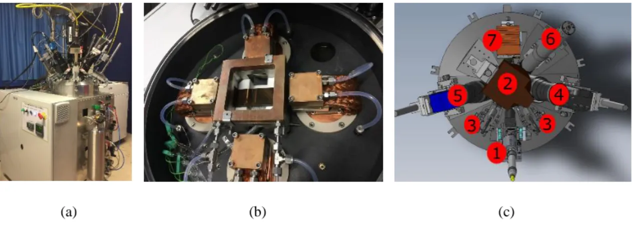
The so-called FLASH facility has been developed to perform thermal fatigue tests by pulsed laser or helium jets (Fig. 1(a)). The specimen is put inside an airtight chamber (Fig. 1(b)) filled with helium to eliminate subsequent oxidation that would alter the surface emissivity, namely, the speckles to enable for DIC analyses, as well as heat exchanges between the specimen and the laser beam (absorptivity) or helium atmosphere (convection).
4
(a) (b) (c)
Fig. 1 (a) Overview of the FLASH facility. (b) Specimen plate inside the inner chamber. (c) Top view of the experimental configuration with its main components (see main text for a detailed description of the components labeled in the CAD
model)
The thermal loadings are performed by a pulsed laser (TruPulse 156, Trumpf, λ = 1064 nm, see Fig. 1(c)-label (1)) on the center area of the specimen at a frequency of 1 Hz. The pulse duration is 50 ms, and the incident pulsed power is adapted to obtain the desired temperature variation on the surface of the specimen.
An IR camera (x6540sc FLIR, 14-bit, cooled indium antimonide detector with full definition: 640 512 pixels, 𝜆 ∈ [3; 5 μm] reduced to 𝜆 ∈ [3.97; 4.01 μm] with an internal germanium filter for high temperature measurements, Fig. 1(c)-label (2)) is used to measure Lagrangian temperature fields and 3D displacement fields with a high magnification lens allowing for a pixel resolution of 15 µm. The IR camera is normal to the sample surface. Two fast pyrometers (KGA740-LO, 𝜆 ∈ [1.58; 2.2 𝜇𝑚], at 1.2 kHz, Fig. 1(c)-label (3)) are used to measure and monitor within the impacted zone the temperature variation on a 2.5 mm wide area. The first visible light camera (MIRO M320S, Vision Research, 16-bit, full definition: 1920 1200 pixels, Fig. 1(c)-label (4)) with a pixel resolution of 10 µm corresponds to the second device of the multiview system. Another visible light camera was recently introduced as the third device (pco.edge, 16-bit, definition: 2560 2160 pixels, Fig. 1(c)-label (5)) with a smaller pixel resolution of 6.5 µm (referred to as PCO in the following). A high power LED projector (Fig. 1(c)-label (6)) provides the necessary light for both visible light cameras. The laser tube is inclined to reflect the incident beam onto a calorimeter (Fig. 1(c)-label (7)) to evaluate the absorptivity of the surface at the laser wavelength. Even though the polished surface is assumed to be specular, the inner walls of the chamber were coated by a high emissivity black paint to absorb the diffusive reflection of the laser flux (Fig. 1(b)). All three cameras are synchronized on the same stroboscopic acquisition signal to compensate for the relatively lower acquisition frequency of the PCO camera, and at the same time, to facilitate the comparison between simulated and experimental thermomechanical fields.
Experimental protocol
The specimens were polished plates made of 316L(N) austenitic stainless steel with dimensions 270 40 7 mm3.
In order to have enough gray level contrast for HMC procedures, and to slightly increase the emissivity of the polished surface, the specimens were heated up to 500°C for 3 days in air to get random pre-oxidation speckles.
5
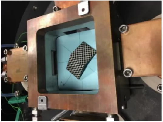
Micro-hardness markers were intentionally added to mark out the area within which laser shocks occur, and to ease the calibration procedure of the HMC procedure.One major challenge is to spatially register images acquired by the three cameras. The 3D target utilized for HMC calibration is placed on the specimen surface in order to preserve a unique reference frame as shown in Fig. 2. The calibration target is an “open-book” made of aluminum alloy, which was used for the calibration of several stereo-systems: first, for an ultrahigh speed experiment [43], and then for the stereorig of the first configuration of the FLASH facility [41]. Its size is 30 30 14 mm3, and the opening angle is 132°. The pattern is made of regular
white and black squares of size 2.5 2.5 mm2 engraved by laser. The position and orientation of the calibration
target have been optimized in order to capture the whole laser beam in the Region of Interest (ROI) defined by the area covered by nine squares in central part (Fig. 4). In the following, the presented thermomechanical fields are those of a common 6.8 7.5 mm2 ROI located in the center of the specimen.
Fig. 2 Calibration “open-book” target placed on the specimen
In order to ensure accurate temperature measurements, the calibration of the IR camera and the pyrometers is necessary. The IR camera was provided with built-in calibration files that allow for accurate measurement regardless of any variation of room temperature. The maker hence performed Non Uniformity Correction (NUC) and calibration by positioning the IR camera in front of several black bodies from inside a temperature-controlled chamber. An in-house verification of maker calibration on a cavity black body showed that the built-in files were faithful. The integration time was then optimized for the present experiments by considering two factors: (i) maximize the signal to noise ratio, (ii) ensure the desired temperature range without saturating the detector. The camera maker software then allowed to automatically identify the apparent emissivity of each specimen based on the measurement of its temperature with the regulation K-type thermocouple implemented at half of its thickness. Each specimen was hence continuously heated in Helium atmosphere to reach the lower bound of the temperature range (400 – 600°C) covered by the thermal fatigue experiments, and the change of emissivity values measured by IR camera through this specific temperature range could be measured by prescribing steady state temperatures with increasing steps of 25°C. It appeared that the value of emissivity did not stay constant through the considered temperature range, which eventually prevented the authors from using camera maker calibration to measure actual temperature variations in thermal fatigue experiments (NUC files are however kept).
6
A specific calibration was then performed on each specimen in the temperature range 400-600°C, following a general form of Planck’s law to relate the output signals and the sought temperatureln(1 ) B T A Signal offset (1)
where T is the absolute temperature of the surface (considered equal to that measured by the K-type thermocouple during the steady state steps), Signal represents the digital levels (DL) for the IR camera or the output voltage of the pyrometers. For the IR camera, the emissivity
cam was determined at 400°C with the camera maker calibration. The calibration then consists in identifying the three parameters A, B and offset so that the difference between experimental and predicted Signal be minimum on all steps. For the investigated sample, the least squares regression yielded Acam 8.15 105DLs, Bcam 3475K , offsetcam 2682DLs. The same Eq. (1) was alreadyused to perform the calibration of the pyrometers facing a cavity blackbody on a larger temperature variation range [200-700°C]. The calibration parameters were Apyro 1.59 107mV, Bpyro 7260K , offsetpyro 3.5mV . The
emissivity of the specimen
pyro was then determined for each prescribed temperature step, and this value only increased from 0.253 to 0.26 in the [400-600°C] temperature range. Considering a constant value for the emissivitypyro
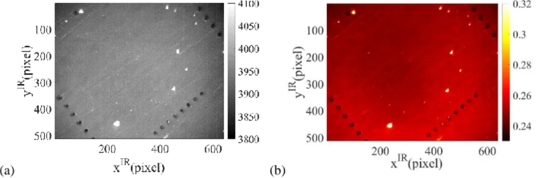
on this domain, namely the one identified at 400 °C, the largest error on temperature measurement was only 3°C at 600°C. This error was considered negligible, and thus the value determined at 400°C will be used for monitoring the temperature field of the central part of the specimen during fatigue tests.One image of the IR camera equipped with the ×1 magnification lens is shown in Fig. 3(a) for one sample heated up to 400°C. Since the temperature of the heated sample is much higher than the environment, the luminance owing to the reflection of the surrounding is negligible compared to that of the sample, even for moderately low values of emissivity. Therefore, the reflection of camera sensor on the sample, which is known as “Narcissus effect” [27][44], was not observed in the reported tests. The speckle showed a globally uniform field. The randomly distributed bright spots were obtained from pre-oxidation. If the temperature of the whole scene is assumed to be exactly equal to 400°C, Eq. (1) can be used to identify an emissivity field
cam instead of the constant spatial average used in the calibration process. This emissivity field
cam, which is plotted in Fig. 3(b), is uniform except at the corners of the IR image where the regularly spaced spots are micro-hardness marks. Several machining lines are also visible.Optical artifacts in IR measurements were evaluated by integrated DIC [45]. It was shown that the distortion amplitudes were higher near the boundaries of the images. In the current work, in order to minimize the influence of optical artifacts, the camera was positioned normal to the sample surface and only the central part of IR images was chosen as the ROI (Fig. 5a). Furthermore, the laser pulses induce very small displacement amplitudes (few tenths of one pixel), which means that the distortion effects will not express themselves very much. Hence, the optical effects were assumed to be negligible.
7
(a) (b)
Fig. 3 Sample surface heated to 400°C in Helium atmosphere (a) observed by the IR camera equipped with the G1 lens (expressed in digital levels) and (b) the apparent emissivity field
Before performing thermal fatigue tests, the austenitic stainless steel plate (Fig. 1(b)) was continuously heated by Joule effect until its center reaches 400°C, a temperature (controlled by a K-type thermocouple) representative of the initial temperature of primary circuits of SFRs. Then laser pulses were activated by adjusting the power density to reach a temperature variation equal to 180°C. A stroboscopic acquisition was performed in order to measure the displacement and temperature fields at the same time. It triggered each laser pulse at a constant rate as well as the start of any sequence of camera acquisition corresponding to the activation of a new laser pulse [9]. All three cameras were synchronized with an acquisition frequency of 60 Hz. Three images were acquired for the first 50 ms of a thermal loading cycle during which the laser pulse was activated. With current experimental settings, a unique virtual cycle can be reconstructed from 10 real cycles (Fig. 23(a-b)), thereby increasing the camera acquisition frequency to 600 Hz.
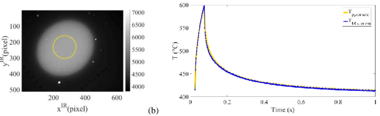
Comparing then the temperatures measured on the laser beam axis by the pyrometer and the IR camera, a significant difference could be observed at the end of the laser pulse, namely, when the temperature was the highest. The camera measured a value 20°C lower than the pyrometer with the calibration parameters identified in the steady step procedure. This difference is the signature of the so-called Size-of-Source Effect (SSE) [46]. Due to imperfections of the G1 lens, the radiation thermometer on the central area of the camera detector is affected by the surrounding area. In the present case, the activation of the laser beam induces high levels of IR flux on only a reduced central area of the IR camera sensor surrounded by a “cold” region, as shown in Fig. 4(a), contrary to the calibration procedure where the camera was exposed to a uniform and large area that emits high levels of IR flux when the sample reaches 600°C. The calibration parameters were thus adapted to the measurement of temperature on large uniform areas such as those observed at the end of a pulse period, just prior to the start of a new laser pulse, but they were not well adapted to measure the temperature on the area impacted by the laser beam. However, since the pyrometers measure the temperature on a central area (1.25 mm radius) completely covered by the laser beam as indicated in Fig. 4(a), there is no difference between the calibration and the thermal fatigue configurations for this device, namely no SSE. Consequently, the temperature measurements performed by the pyrometer with the values of calibration parameters identified in the calibration configuration were considered accurate. The last step of the IR camera calibration is then to re-identify the parameters of Eq. (1) by minimizing the difference between the temperature measured by the pyrometer and those on the laser beam axis by the IR camera during one loading cycle (see Fig. 4(b)). The final set of calibration parameters used to measure temperature fields during cyclic thermal loadings is Acam 2.98 105DLs, Bcam 2753K , offsetcam 2540DLs.
8
(a) (b)
Fig. 4 (a) Sample surface heated by laser beam observed by the IR camera and the central area measured by pyrometers indicated by the yellow circle. The results are expressed in DL. (b) Temperature history during one cycle measured by the
pyrometers (in yellow) to calibrate the IR camera (in blue) affected by the Size-of-Source Effect
In order to maintain the walls of the chamber at room temperature, a forced (convective) cooled helium flux was applied during the tests. The convection in the helium atmosphere results in thermal gradients between the hot sample and the cold camera sensors, and these gradients induce variations of the refractive index and may influence the optical path of cameras, which is the so-called heat haze effect [47]. For all discussed images, the helium flow was shut down in order to avoid spurious effects generated by convection.
NURBS description of the observed surface
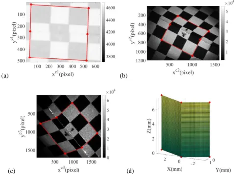
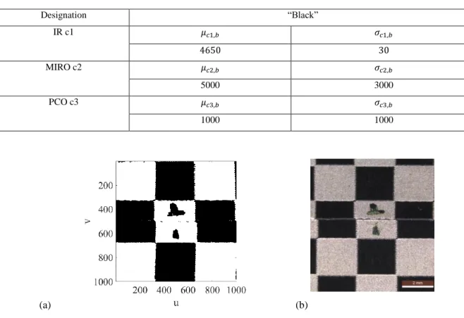
The observed surfaces (that of the calibration target and of the specimen) are described by their CAD model. As shown in Fig. 5, each imaging modality gives differing appearances of the calibration target due to the different wavelength ranges and sensitivities of the chosen measurement approach, though globally the main features (i.e., “black” and “white” squares, which are inverted in the IR camera with respect to visible light cameras due to the different emissivity of working wavelengths) of the target can still be recognized. The numerical model is the master information that is decorated by the specific texture captured by multiple imaging modalities.
B-Spline and Non-Uniform Rational Basis Spline (NURBS) functions have been proposed to measure displacement and displacement gradients by 2D DIC [48][49]. More recently, they were used in stereocorrelation [35][36] and multiview registrations [50]. They will also be utilized herein to define the geometry of the calibration target, that of the surface of interest, and the kinematic parameterization of the displacement fields. A NURBS representation of the surface 𝑿(𝑢, 𝑣) = (𝑋, 𝑌, 𝑍) is defined in the parametric space (𝑢, 𝑣) as [51]
, , 0 0 , , 0 0 ( ) ( ) ( , ) ( ) ( ) P X m n i p j q ij ij i j m n i p j q ij i j N u N v w u v N u N v w
(2) with9
1 ,0 1 0 :1 , ( ) 0 i i i u u u u N u otherwise (3)and 𝑢𝑖 are the components of the knot vector
1 , , 1 1, 1 1 1 ( ) i ( ) i p ( ) i p i p i p i p i i p i u u u u N u N u N u u u u u (4)
where 𝑁𝑖,𝑝 are mixing functions, 𝑷𝑖𝑗 the coordinates of control points of the surface, 𝑤𝑖𝑗 the corresponding weights, (𝑚 × 𝑛) the number of control points, and (𝑝, 𝑞) the degrees of the surface (here 1).
The surface of the open-book calibration target is composed of two NURBS surfaces. In the present case, all weights are equal to 1, which reduces the NURBS surface to Bézier patches. The geometric continuity is then defined by the fact that the two surfaces coincide by sharing the common control points (C0 continuity) but not C1
to allow for slope discontinuity.
(a) (b)
(c) (d)
Fig. 5 Open-book calibration target captured by (a) the IR camera (denoted as c1), (b) the first visible light camera MIRO (denoted as c2), (c) the second visible light camera PCO (denoted as c3), and the corresponding ROIs (see red boxes in all
above images). (d) NURBS model of the calibration target with 6 control points (red solid circles)
Calibration phase
The calibration of the multiview system consists in finding the projection matrices from the 3D physical coordinates to the 2D sensor frame for each of imaging modality
M X ci ci ci ci ci ci l x l y l (5)10
where [𝑴𝒄𝒊] is the 3 x 4 projection matrix with respect to the numerical model, {𝑿̅}𝑡= {𝑋, 𝑌, 𝑍, 1} the corresponding homogeneous coordinates of any 3D point in the parametric space, 𝑥𝑐𝑖 and 𝑦𝑐𝑖 the pixel coordinates, and 𝑙𝑐𝑖 the scale factor for each camera.Once the projection matrices are determined, the pixel images acquired by all the cameras can then be interpolated in the parametric space of the NURBS model. One possible formulation to estimate [𝑴𝒄𝒊] is to perform a global approach [50] based on camera pairs observing the common surface
3 2 2 1, , , , , x M x M cam n ci ci ci cj cj cj i j i ROI f u v f u v
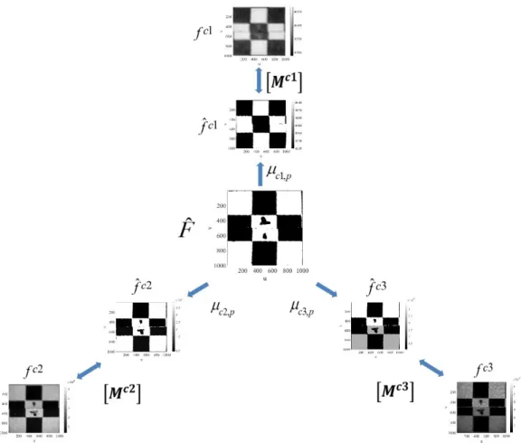
(6) where 𝑓𝑐𝑖 denotes the picture acquired by camera 𝑐𝑖. Note that a numerical operation needs to be performed on the digital level response of the IR camera since the natural “white” and “black” hues are inversed in the IR camera with respect to visible light cameras due to the difference of emissivity. Moreover, since the dynamic ranges of the three cameras are quite different (Fig. 5), the global minimization of Equation (6) can be difficult to cope with three stereoscopic combinations.Another natural choice is to perform the registration of each camera with one unique reference image, which is obtained by averaging over all images observed over the same surface [50]. In the cited work, all four cameras were of the same modality and type, and hence the images were similar from one to any other. Although different contrasts may be challenging, the idea to define a unique reference image to access the coincidence of three different images appears as a feasible solution. As proposed in Refs. [52], [53], the multimodality registration is constructed based on artificial reference images 𝑓̂𝑐𝑖, which are obtained by geometric segmentation of material points of the calibration target for every modality sharing the same information of a unique reference frame, 𝐹̂. Therefore, a global formulation is needed in which the sum of squared differences expressed in the parametric space is minimized with respect to each unknown projection matrix [𝑴𝑐𝑖] over the whole ROI
2
ˆ
2(
ci(
x
ci( , ,
M
ci))
ci)
ROI
f
u v
f
(7) The proposed formulation is summarized in Fig. 611
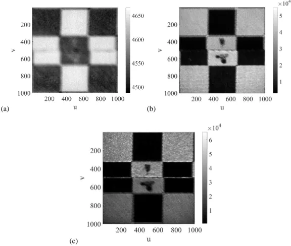
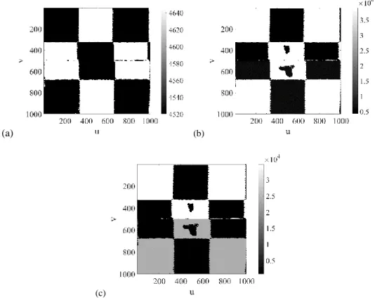
Fig. 6 Determination of the projection matrices via global multiview correlation based on the unique reference 𝐹̂An initial guess is needed to estimate the projection matrices by performing global SC between two cameras. Even though different gray level distributions occur, such a challenge can be overcome [41] by considering the digital / gray level relaxation between the IR camera and visible light cameras by selecting low order polynomials. At convergence of the SC algorithm, the 3D surface is projected onto the 2D space using the determined projection matrices. The pictures in Fig. 5 can be interpolated to create corresponding sub-pictures in the parametric space. Figure 7 illustrates the average of these parametric sub-pictures obtained from two stereoscopic combinations involving the specific camera. Globally, the main features of the nine squares are well captured while some slight mismatches still exist, see for example Fig. 7(b) and Fig. 7(c) where a displacement of about 25 pixels can be observed along the v direction. Hence, there is a need for better calibrating the projection matrices. Even if the averaged determination is not optimal, it still provides a reasonable estimate of the projection matrices in order to initialize the minimization of Equation (7).
12
(a) (b)
(c)
Fig. 7 Images of the calibration target obtained by averaging sub-images determined by projection matrices from stereoscopic combination results for the (a) IR image, (b) MIRO image, (c) PCO image in the parametric space (u, v)
13
Determination of
𝒇̂
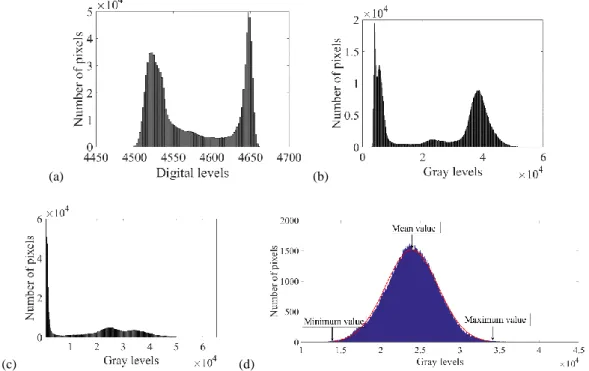
𝒄𝒊Images mainly contain 2 phases, “white” and “black” hues in the squares, and the black markers “T” and “I” in the central white square (Fig. 5), which were intentionally added in order to identify the position of the calibration target in the wide field of view during the test. Images are analyzed with their digital / gray level histograms shown in Fig. 8. The digital / gray levels in the ROI belong to “white” or “black” categories for all three images.
(a) (b)
(c) (d)
Fig. 8 Digital / gray level histogram of ROI (a) IR image, (b) MIRO image, (c) PCO image. (d) “White” in lower half of PCO image
During image acquisition, noise (i.e. shot noise, dark current, read out noise, illumination fluctuations) occurs. For every pixel in the ROI, the digital / gray level follows a specific Gaussian distribution decorated by acquisition noise. Therefore, it is proposed to consider the distribution of gray levels 𝐺𝐿 (the same symbol to represent digital levels DL for IR image in following formulas) to determine, for every pixel in every image, whether it belongs to white or black phases
,
2 , , 2 , , 1 | , exp 2 2 ci p ci p ci p ci p ci p GL GL (8)where 𝛼 is the Gaussian distribution of 𝐺𝐿 at one single parametric position with mean 𝜇𝑐𝑖,𝑝 and variance
𝜎
𝑐𝑖,𝑝2, and 𝑝 “white” or “black” phases. In the present case, the images contain roughly two phases (“white” and“black”), which are separable. One practical way of segmenting the phase is to consider the probability density at each pixel with the contribution from every image, 𝑐𝑖, for the binarization
, ,
( ) ( | ci p, ci p)
ci
14
Since “white” values vary spatially much more significantly (i.e., two peaks in histograms with centroids largely different, see Fig. 8) than the “black” levels in visible light images, the “black” probability is determined with the parameters reported in Tab. 1. The threshold to distinguish black from white is chosen to obtain the details of the calibration target observed by optical microscopy (Fig. 9), like the saw tooth pattern engraved by laser. Hence this approach leads to the (“white” or “black”) segmentation of images into phases, for each pixel in the parametric space, which refer to a single intrinsic reference frame 𝐹̂ combining all the available information from the multimodal images.Tab. 1 Evaluation of the Gaussian parameters of the “black” phase for images shown in Fig. 7, the black is denoted as “b”
Designation “Black” IR c1 𝜇𝑐1,𝑏 𝜎𝑐1,𝑏 4650 30 MIRO c2 𝜇𝑐2,𝑏 𝜎𝑐2,𝑏 5000 3000 PCO c3 𝜇𝑐3,𝑏 𝜎𝑐3,𝑏 1000 1000 (a) (b)
Fig. 9 (a) Intrinsic geometric reference frame 𝐹̂. (b) Calibration target observed by optical microscopy
With respect to the light source position, the “white” and “black” appearance can even be subdivided into “bright” or “dark” in visible light images (see multiple peaks in Fig. 8(b-c)). As shown in Fig. 8(d), the “white” squares in the lower half of the PCO image (Fig. 7(c)) follow a normal distribution from which the Gaussian parameters are deduced. Additionally, one needs to mention that the involved pixels were carefully chosen by avoiding the transition zones between “black” and “white” hues to obtain separate Gaussian distributions. By analyzing the gray level distribution of every phase for each visible light camera according to the pixel position, the results are summarized in Tab. 2.
15
Tab. 2 Gaussian parameters of each phase for images shown in Fig. 6, the “white” zone is denoted as “w”, and the black isdenoted as “b”. For visible light images the upper half is denoted as “𝑤1” and “𝑏1”, the lower half is denoted as “𝑤2” and “𝑏2”
Designation “White” “Black”
IR c1 𝜇𝑐1,𝑤 𝜎𝑐1,𝑤 𝜇𝑐1,𝑏 𝜎𝑐1,𝑏 4520 45 4650 30 MIRO c2 𝜇𝑐2,𝑤1 𝜎𝑐2,𝑤1 𝜇𝑐2,𝑤2 𝜎𝑐2,𝑤2 𝜇𝑐2,𝑏1 𝜎𝑐2,𝑏1 𝜇𝑐2,𝑏2 𝜎𝑐2,𝑏2 3.86 × 10⁴ 6000 3.90 × 10⁴ 1.16 × 10⁴ 4200 3500 5850 3000 PCO c3 𝜇𝑐3,𝑤1 𝜎𝑐3,𝑤1 𝜇𝑐3,𝑤2 𝜎𝑐3,𝑤2 𝜇𝑐3,𝑏1 𝜎𝑐3,𝑏1 𝜇𝑐3,𝑏2 𝜎𝑐3,𝑏2 3.48 × 10⁴ 1.7 × 10⁴ 2.40 × 10⁴ 9.95 × 10³ 1285 1200 760 700
Once the intrinsic reference frame 𝐹̂ is defined, the noise free artificial reference image for every camera 𝑓̂𝑐𝑖 is constructed by coloring the corresponding pixel with the centroid value reported in Tab. 2 as shown in Fig. 10.
(a) (b)
(c)
Fig. 10 Artificial reference image 𝑓̂𝑐𝑖 of (a) IR, (b) MIRO, (c) PCO cameras
As in standard global approaches, a modified Newton-Raphson iterative scheme is used to minimize the sum of squared differences over the considered ROI accounting for the corresponding 𝜎𝑐𝑖,𝑝 between the digital / gray level images 𝑓𝑐𝑖 and the reference image 𝑓̂𝑐𝑖
2 2 2 , ˆ ( ( ( , , )) ) 2 x M ci ci ci ci eq ROI ci p f u v f (10)
16
In Equation (10), 𝒙𝒄𝒊 denotes the current estimates of the 2D positions of 3D points obtained with the current estimates of matrices [𝑴𝒄𝒊] ,𝜎
𝑐𝑖,𝑝2the variance of the corresponding phase. Consequently, a “pseudo”-displacement is generated with respect to [𝑴𝒄𝒊] so as to reposition 𝑓𝑐𝑖 to be matched with the artificial reference image 𝑓̂𝑐𝑖. In practice, only 11 parameters are sought since the projection matrix is determined up to a multiplicative constant (𝑀3,4𝑐𝑖) for every camera independently, while the three cameras are bound together with the unique reference frame 𝐹̂.
The digital / gray level conservation between the image 𝑓𝑐𝑖 and the unique reference image 𝑓̂𝑐𝑖 is investigated with respect to the estimates of projection matrices [𝑴𝒄𝒊]. The equivalent digital / gray level residual fields are plotted in Fig. 11 for the three modality images. They are expressed in the parametric space of the 3D surface (𝑢, 𝑣). When [𝑴𝒄𝒊] is initialized by the averaged SC results, a clear mismatch is observed with the presence of steps in Fig. 11(a), (c), and (e). At convergence, as shown in Fig. 11(b), (d), and (f), although some bright edges can still be seen, all the initial steps have disappeared.
(a) (b)
(c) (d)
(e) (f)
Fig. 11 Digital / gray level residual field for the determination of the projection matrices. (a) Initial difference and (b) at convergence for the IR camera (RMS values: 2.4 and 1.1 with 25 iterations). (c) Initial difference and (d) at convergence for
the MIRO camera (RMS values: 8.9 and 3.3 with 14 iterations). (e) Initial difference and (f) at convergence for the PCO camera (RMS values: 40.7 and 14.6 with 21 iterations)
17
At the end of the calibration step, the values of root mean square of digital / gray level residuals have all converged to lower levels as shown in Fig. 12, which validates the registration results. The residual level is mainly caused by the fact that the saw teeth of the calibration target are not perfectly reconstructed in 𝐹̂. While the essential feature of the calibration procedure is to reach coincidence of images onto a unique reference frame, such local deviation is acceptable and the registration is deemed successful.(a) (b)
(c)
Fig. 12 Change of root mean square of digital / gray level residuals during the calibration phase for (a) the IR camera, (b) the MIRO camera, and (c) the PCO camera
Displacement measurement due to laser pulse
From the calibration procedure of the multiview system, the projection matrices enable us to perform the transition from the 3D NURBS model of the specimen to 2D sensor planes. By interpolating gray level images in the parametric space, the registration is carried out with these parametric images where the only master information is the 3D NURBS model of the observed surface. In the following, it is assumed that the 3D target used for the calibration phase and the characterized 2D surface share the same reference position as shown in Fig. 13. To measure displacement fields under thermal loadings, the registration algorithm consists in moving the control points of the current surface, which describe the best deformed images with respect to reference images estimated by the nominal surface.
18
HMC is performed by registering all three image pairs in the reference and current configurations by simultaneously minimizing three global residuals, namely, the sum of squared differences in the considered ROI with respect to the motions of the control points 𝒅𝑷𝒊𝒋
3 2 2, ,
, ,
x
P
x
P
dP
cam n ci ci ci ci ij ij ij ci ROIf
u v
g
u v
(11)where 𝑷𝒊𝒋 are the initial positions of the control points of the NURBS surface. The displacement fields are obtained by searching for the incremental motions 𝒅𝑷𝒊𝒋 of the control points in the deformed images 𝑔𝑐𝑖 with respect to the reference images 𝑓𝑐𝑖. A Newton-Raphson algorithm is implemented to minimize the above correlation residual. The linearized system to solve reads
H dp b (12) with the HMC matrix
x D P ci ci ci ij ij f (13)
H 3
D D cam n T ci ci ci
(14) where the unknowns (i.e., 3 × 16 coordinates defining the 16 control points) are incrementally determined as
dp
dPij (15)and the HMC vector
b 3
D
cam n T ci ci ci ci f g
(16) The reference image is defined as that captured just before the activation of the laser pulse, and the deformed image, as that captured at the end of the laser pulse when the temperature variation is the highest. Three pairs of reference and deformed images interpolated in the parametric space are shown in Fig. 14. For these images, the contrasts of the specimen surface are quite different, due on the one hand to the difference in wavelength domains between IR and visible images, and on the other hand to the relative orientation of the visible light cameras with respect to the light source (Fig. 1(c)-label (6)). The IR camera is more sensitive to oxides, the MIRO camera shows a better detection of the machining roughness, and the PCO camera enables the micro-hardness marks to be better detected. The visible light images show an identical contrast before and after the activation of the laser pulse. Conversely, the large temperature variation (180°C) of the specimen surface induced by 50 ms constant heating with the laser beam introduces a significant gray level variation in the deformed IR image (Fig. 14(b) compared to Fig. 14(a)).19
(a) (b)
(c) (d)
(e) (f)
Fig. 14 Reference images (just before the activation of the laser pulse) and deformed images (at the end of the laser pulse) in the parametric space. (a-b) IR images, (c-d) MIRO images, and (e-f) PCO images (limited to 30% of raw dynamic range in
20
Correction of IR frames
From the above discussion, it is important to note that the raw deformed IR images cannot be successfully used in the HMC algorithm without digital level corrections (see Fig. 14(a-b)). The correction is performed with a global and regularized DIC approach [32]. The digital level conservation is recovered by adding brightness and contrast corrections
1 1 ( )x a( )x 1 ( )x x u x( ) c c f b g (17) where 𝒖(𝒙) is the 2D displacement field, 𝑎(𝒙) the brightness correction, and 𝑏(𝒙) the contrast variation. By performing regularized T3-DIC (i.e., using a mesh made of 3-noded (T3) triangular elements) between the reference and deformed IR images, all these fields are obtained. Figure 15(a-b) shows the residual maps before and after taking into account the brightness and contrast corrections. Thanks to the digital level correction, the initial residual between the reference and deformed images is reduced from 22.6% to 0.3% of the dynamic range. At convergence, the deformed image 𝑔𝑐1 is corrected by the 𝑎(𝒙) and 𝑏(𝒙) fields representing the temperature variation (Fig. 15 (c))
1 1 ( ) (1 ( )) x x x x c c corrected g a b g (18) In the present case, this correction allows us to retrieve similar digital levels in the HMC formulation. Afterward, three pairs of images are considered to measure 3D displacement fields induced by the laser pulses.(a) (b)
(c)
Fig. 15 Comparison between the initial residual map expressed as percentage of the dynamic range of the deformed image without (a) and with (b) brightness and contrast corrections (RMS values: 22.6% and 0.3%, respectively) (here Fig. 15(b)
limited to 50% of dynamic range of Fig. 15(a)). (c) Corrected deformed IR image (limited to 15% of dynamic range of Fig. 14(a) in order to reveal the speckle left for DIC analyses)
21
Uncertainty quantifications
One conventional method, which is based on the rigid-body motions to investigate the measurement errors related to DIC [54], is not applicable due to the experimental environment. Therefore, one way proposed herein to estimate the measurement uncertainties is to exploit the images acquired during the initial heating up phase. Ten images were acquired simultaneously during this steady state by each camera with an acquisition frequency of 60 Hz. HMC analyses are conducted to measure the displacement fields with these images. For example, the first images are assumed as the references for each camera, and the subsequent images as the deformed ones. Then the same procedure is applied correlating this time the second images with the following ones, and so on. In total 45 measurements are obtained. One example of such displacement field measurement is shown in Fig. 16 where the reference configuration is the fifth images and the deformed configuration is the sixth images. Despite the fact that the sample is stabilized at 400°C with no expected motion, the HMC algorithm estimates displacements of micrometric order. Considering that in reality no displacement took place, the statistics of these displacement fields reveal the global uncertainty of the measurement. It includes various sources, such as machine vibration, noise during image acquisition and digitization as well as those related to the HMC algorithm.
(a) (b) (c)
Fig. 16 Example of displacement fields (expressed in µm) of the specimen stabilized at 400°C (5th reference images, and 6th
deformed images). (a) UX, (b) out of plane UY, and (c) UZ
To quantify them, the standard deviation of the 45 displacement measurements is calculated at each evaluation point in the parametric space (Fig. 17). The average values are 0.74 µm, 0.79 µm and 0.73 µm for 𝜎(𝑈𝑋), 𝜎(𝑈𝑌) and 𝜎(𝑈𝑍) respectively. The uncertainties on in-plane displacements (𝑈𝑋 and 𝑈𝑍) are slightly lower than those for out-of-plane displacements (𝑈𝑌), but, in order to be conservative, the uncertainty level can be schematized as of order 0.8 µm in all directions. It is also to be noted that these point-wise uncertainties do not do justice to the fact that these fluctuations are strongly correlated in space because of the NURBS basis used.
(a) (b) (c)
Fig. 17 Standard displacement uncertainties (expressed in µm) associated with 45 displacement measurements when the applied temperature is stabilized at 400°C. (a) UX, (b) out of plane UY, and (c) UZ
Since the same NURBS basis functions are used for surface shape and displacement fields, the so-called isogeometric collocation method [55] is applied to compute the deformation gradient with the two in-plane
22
displacement components plotted in Fig. 17(a,c). With the same method, the maps of standard deviations of the 45 in-plane strain measurements in the parametric space are plotted in Fig. 18. The average values are 1.7 × 10⁻⁴ and 8 × 10⁻⁵ for 𝜎(𝜖𝑋𝑋) and 𝜎(𝜖𝑍𝑍) respectively.
For the temperature measurement, the same method is applied to 10 IR images when the plate is stabilized at 400°C. One measured temperature field is shown in Fig. 19(a), and the map of standard deviations of the 10 temperature measurements in the parametric space is plotted in Fig. 19(c). The average value is 0.02°C for 𝜎(𝑇). Except for the presence of oxides for which the emissivity is higher as shown in Fig. 19(b), the temperature measurements are quite stable.
(a) (b)
Fig. 18 Standard strain uncertainties associated with 45 in-plane strain measurements when the applied temperature is stabilized at 400°C. (a) 𝜖𝑥𝑥, (b) 𝜖𝑧𝑧
(a) (b) (c)
Fig. 19 (a) Temperature field (expressed in °C) stabilized at 400°C (b) corresponding emissivity map, and (c) corresponding standard temperature uncertainty (expressed in °C)
23
Results
In all the cases reported herein, the convergence criterion was written as the standard variation of the norm of the incremental correction vector {𝒅𝑷} with a threshold of 10−6 𝑚𝑚. Since the dynamic range of IR images is much lower than that of visible images as shown in Fig. 14, the images are normalized in order to take account of all three modalities’ contributions to the global linearized system expressed in Eq. (11). The number of iterations needed to achieve convergence was 35. Figure 20 shows the raw differences ((a)-(c)-(e)), and the residual maps at convergence ((b)-(d)-(f)) of three pairs of images. The main features are no longer detectable (at least on the residual maps of visible cameras). For example, the oxides, the machining roughness and micro-hardness marks are erased in IR, MIRO and PCO residual maps respectively, which means that the overall registration and the correlation results are trustworthy.
(a) (b)
(c) (d)
(e) (f)
Fig. 20 Residual maps in the parametric space and RMS value expressed in percentage of the digital / gray level dynamic range. (a) Initial IR residual 𝜂𝑐1= 0.22%, (b) at convergence 𝜂𝑐1= 0.20%. (c) Initial MIRO residual 𝜂𝑐2= 1.16%, (d) at
24
The Lagrangian temperature field measured by the IR camera is shown in Fig. 21(a), which corresponds to the digital level correction reported in Fig. 14(b). The 3D mechanical response of the material under such thermal loading is illustrated in Figs. 21(b-d). The in-plane displacement fields describe biaxial expansion and the out of plane component shows a hump at the center of the laser beam, which follows well the temperature distribution.(a) (b)
(c) (d)
Fig. 21 Thermomechanical fields measured via HMC. (a) Lagrangian temperature field (expressed in °C) at the end of laser pulse. Corresponding UX (b), out of plane UY (c), and UZ (d) fields (expressed in µm)
The in-plane strain fields are plotted in Fig. 22. The amplitudes are close to the expected levels, namely, less than 0.1% at the end of the laser pulse.
(a) (b)
25
A stroboscopic acquisition was performed to trigger not only each laser pulse at a constant rate but also the start of every acquisition sequence of the three cameras.To evaluate the influence of the number of degrees of freedom, the displacement fields corresponding to the maximum temperature variation during one stroboscopic acquisition were measured. The average values of the standard deviation maps of the 10 displacement measurements were then compared. The uncertainty of the out of plane displacement fields reached a value of 0.8 µm, 0.8 µm, 0.9 µm and 1.6 µm for 4, 9, 16, 25 control points, respectively. When the number of control points was low (i.e., 4 and 9), the distribution of displacement fields (i.e., in-plane biaxial expansion state and hump for out-of-plane component as illustrated in Fig. 21) were not well described even though the amplitudes of displacement fields were close to those obtained with a higher number of control points. It is mainly due to an over-reduction of kinematic degrees of freedom in the impacted zone when only the vertices are defined with fewer control points. Hence the most satisfactory compromise was reached for 16 control points between these two conditions.
Based on the current parameters of laser pulse (i.e. 1 Hz frequency with 50 ms duration) and on the minimum value of the acquisition frequency of three cameras (i.e. 60 Hz to synchronize the three cameras), one unique (virtual) cycle can be reconstructed with 10 successive cycles after putting the 600 images acquired by each camera in the appropriate order (that of the phase). An example of the output of such a reconstruction is presented in Fig. 23 where the change of temperature measured in the center of the laser beam by the IR camera is shown for 10 successive real cycles as well as for the reconstructed stroboscopic (virtual) cycle. To track the 3D kinematic fields during one real thermal loading cycle, the last image prior to the start of a new laser pulse is set as the reference configuration to which all subsequent 59 images are correlated by performing HMC analyses. The HMC measurements of the kinematic responses in the center of the laser beam from the 1,800 images acquired by the three cameras during 10 real cycles are then plotted after stroboscopic reconstruction in Fig. 23(c) for the out of plane displacement, and Fig. 23(d) for the normal in-plane strains.
26
(b)(c)
(d)
Fig.23 Time histories of (a) temperature on the sample surface and in the center of the laser beam measured during 10 real cycles. (b) Stroboscopic reconstruction of 1 virtual cycle. Comparison between experimental measurements reconstructed by 10 real cycles via HMC (solid symbols) and 3D numerical simulations (solid lines) for (c) out of plane displacement and (d) in-plane strains at the same location
It is observed that these kinematic measurements are noisy. In order to estimate the uncertainty in this specific test configuration (rather than in the optimal one where the plate was kept at a constant temperature without any laser pulse), a statistical analysis is performed on the last 0.2 s of all 10 cycles, which corresponds to 0.2 s of acquisition at 600 Hz, where the temperature can be considered as stabilized at around 414°C. During this steady state part of the thermal cycle, the standard deviations of the measurements are 1°C, 1.2 µm, 2.0 × 10⁻⁴ and 9.5 × 10⁻⁵, compared to the standard uncertainties of 0.02°C, 0.8 µm, 1.7 × 10⁻⁴ and 8 × 10⁻⁵ during the initial state at
27
400°C, for the temperature, out of plane displacement 𝑈𝑌, in plane normal strains 𝜖𝑋𝑋 and 𝜖𝑍𝑍 respectively. It shows that the uncertainties under real experimental conditions for thermal fatigue tests are only slightly higher than the standard uncertainties. Thus the HMC measurements can be considered as trustworthy despite the presence of noise.The discussed images were acquired during the very first stage of a fatigue test. Three-dimensional finite element simulations were carried out with the assumption that the thermal and mechanical loadings were uncoupled since the self-heating due to plastic deformation was negligible compared to the incident laser power absorbed by the material [9][10]. First, the thermal analysis was carried out to describe the conductive and convective heat transfer processes. The volumetric source corresponding to the Joule effect was calibrated to obtain a stable initial temperature of 400°C at the center of specimen. The spatial density of laser flux was described by a super Gaussian profile where the shape parameters were identified by comparing experimental (as shown in Fig. 21(a)) and numerical temperature fields from a thermal FE model updating procedure. Once the cyclic history of temperature at the shocked center was stabilized, the temperature field was inserted into the thermomechanical calculation to compute the mechanical response described by a nonlinear kinematic hardening law where the parameters of each kinematic variable were calibrated on push-pull cyclic tests at 400°C and 500°C [56]. Other thermophysical parameters (e.g. thermal conductivity, specific heat capacity, coefficient of thermal expansion, Young’s modulus) were chosen from data reported in the French design code RCC-MRx [57].
The histories of out-of-plane displacement and eigen strains experimentally measured via HMC in the central zone of the surface impacted by the laser spot are then compared with those obtained via 3D thermomechanical FE simulations in Fig. 23(c-d), respectively. A higher scatter is observed for the strains in the X-direction compared to the Z-direction, which is consistent with the standard uncertainties that are higher in the former direction. In addition, the measured out of plane displacement 𝑈𝑌𝐻𝑀𝐶 shows a better agreement with simulation results compared to the in plane strains. The measured strain levels are higher than the simulation results, which may be caused by the simplification of the numerical model. Thanks to the sensitivity analyses of the parameters of thermomechanical model applied herein, the in-plane strains are much less sensitive to boundary conditions and model parameters while the out of plane kinematic responses show a higher sensitivity with 10% variations [56]. Globally the tendency of the simulated mechanical response is in good agreement with HMC measurements along the principal directions of the specimen surface. In particular, the measurements show the same order of magnitude as the numerical predictions. Hence, these two approaches are consistent.
To compare in a more quantitative way the simulation results and the HMC measurements at the same time, the simulation results are interpolated at the experimental time steps. The RMS difference between the measured simulated temperature is equal to 7.2°C, to be compared to 1°C uncertainty. The RMS difference between the measured 𝑈𝑌𝐻𝑀𝐶 and interpolated simulation 𝑈𝑌𝐹𝐸𝐴 is equal to 1.23 µm; the corresponding uncertainty being equal to 1.2 µm, the RMS difference is within the uncertainty. For the normal strains, the RMS differences are equal to 2.2 × 10⁻⁴ and 1.2 × 10⁻⁴ along the X- and Z-directions, respectively. Compared to the strain uncertainties, the RMS difference is on average 20% higher. Given the complexity of the experiment and the fact that a thermomechanical model had to be updated in order to describe the boundary conditions of the thermal fatigue test, the whole procedure is deemed fully validated. In particular, HMC is shown to be feasible and validated for measuring micrometer displacements, 100 µ-strains, and temperatures within one Celsius degree.
28
Conclusion and Perspectives
In this paper, full-field 3D thermomechanical measurements were performed in-situ on an austenitic stainless steel plate under laser shocks using an isogeometric hybrid multiview correlation (HMC) algorithm. Working in the NURBS parametric space of the 3D surface allows different image definitions, modalities and resolutions to be registered. One beneficial outcome of such challenging difference is that the calibration phase is performed by defining a unique reference frame based on the information shared by multimodal images of the calibration target. The Lagrangian temperature fields, 3D displacement fields and 2D strain fields were measured for ten cycles of thermal loading.
The measurement errors were evaluated by measuring the temperature and kinematic fields when the specimen surface was stabilized at 400°C before the fatigue test. Submicrometric uncertainties were obtained for displacement measurements. Sub-100 µ levels were achieved for the in-plane strain components. During thermal fatigue tests, the thermomechanical measurement uncertainties were only slightly higher than the previous uncertainties (i.e., on average only 16% higher than the kinematic standard uncertainties, 1°C compared to 0.02°C standard uncertainty for temperature data). The comparison between the experimental measurements with thermomechanical FE simulations shows a very good agreement (i.e., only 20% higher than the kinematic measurement uncertainties, 7.2°C deviation compared to the temperature variations as high as 180°C).
All these results prove the feasibility of and validate HMC analyses with two visible light cameras and one IR camera. The next steps aim to fully exploit the abundant information provided by the combination of the three cameras. The IR camera measures the thermal loading signal with significant digital level changes. The temporal modes extracted from IR camera measurements can directly serve to filter out the above mentioned acquisition noise. Such spatiotemporal regularization approach may greatly improve the signal-to-noise ratio for the present measurements[47].
When the differences between the reference and deformed images are erased to measure displacement fields, the correlation residual field proves to be a powerful tool to detect cracks by exploiting the local deviations to gray level conservation [21], [22]. Every camera shows its own sensitivity to the speckle pattern according to its position and sensor nature. When images during fatigue tests are correlated, the gradual surface relief change due to plastic slip emerging on the free surface is evidenced in the residual map of the PCO camera, and the cracks pop out in the residual map of the MIRO camera. In addition, the presence of cracks locally changes the emissivity of specimen surface, thus the cracks are directly observed in the IR pictures. All these features highlight the potential of HMC to track the crack network formation and propagation in thermal fatigue tests.
References
[1] Fissolo, A., Amiable, S., Ancelet, O., et al. (2009). Crack initiation under thermal fatigue: An overview of CEA experience. Part I: Thermal fatigue appears to be more damaging than uniaxial isothermal fatigue. International Journal of Fatigue, 31(3), 587-600.
29
[2] Fissolo, A., Gourdin, C., Ancelet, O., et al. (2009). Crack initiation under thermal fatigue: An overview of CEA experience: Part II (of II): Application of various criteria to biaxial thermal fatigue tests and a first proposal to improve the estimation of the thermal fatigue damage. International Journal of Fatigue, 31(7), 1196-1210.[3] Le Duff, J. A., Tacchini, B., Stephan, J.M., et al. (2011, January). High cycle thermal fatigue issues in RHRS mixing tees and thermal fatigue test on a representative 304 L mixing zone. In ASME 2011 Pressure Vessels
and Piping Conference (pp. 691-699). American Society of Mechanical Engineers.
[4] Paffumi, E., Nilsson, K. F., & Szaraz, Z. (2015). Experimental and numerical assessment of thermal fatigue in 316 austenitic steel pipes. Engineering Failure Analysis, 47, 312-327.
[5] Taheri, S., Julan, E., Tran, X. V., & Robert, N. (2017). Impacts of weld residual stresses and fatigue crack growth threshold on crack arrest under high-cycle thermal fluctuations. Nuclear Engineering and Design, 311, 16-27.
[6] Metzner, K. J., & Wilke, U. (2005). European THERFAT project—thermal fatigue evaluation of piping system “Tee”-connections. Nuclear Engineering and Design, 235(2-4), 473-484.
[7] Cacuci, D. G. (2010). Handbook of nuclear engineering. Volume I: Nuclear Engineering Fundamentals.
[8] Vincent, L., Poncelet, M., Roux, S., Hild, F., & Farcage, D. (2013). Experimental facility for high cycle thermal fatigue tests using laser shocks. Procedia Engineering, 66, 669-675.
[9] Charbal, A., Vincent, L., Hild, F., Poncelet, M., Dufour, J. E., Roux, S., & Farcage, D. (2016). Characterization of temperature and strain fields during cyclic laser shocks. Quantitative InfraRed
Thermography Journal, 13(1), 1-18.
[10] Wang, Y., Charbal, A., Hild, F., & Vincent, L. (2018). High cycle thermal fatigue of austenitic stainless steel. In MATEC Web of Conferences (Vol. 165). EDP Sciences.
[11] Luong, M. P. (1998). Fatigue limit evaluation of metals using an infrared thermographic technique. Mechanics of materials, 28(1-4), 155-163.
[12] La Rosa, G., & Risitano, A. (2000). Thermographic methodology for rapid determination of the fatigue limit of materials and mechanical components. International journal of fatigue, 22(1), 65-73.
[13] Yang, B., Liaw, P. K., Wang, H., Jiang, L., Huang, J. Y., Kuo, R. C., & Huang, J. G. (2001). Thermographic investigation of the fatigue behavior of reactor pressure vessel steels. Materials Science and Engineering: A, 314(1-2), 131-139.
[14] Wagner, D., Ranc, N., Bathias, C., & Paris, P. C. (2010). Fatigue crack initiation detection by an infrared thermography method. Fatigue & Fracture of Engineering Materials & Structures, 33(1), 12-21.
[15] Plekhov, O., Palin-Luc, T., Saintier, N., Uvarov, S., & Naimark, O. (2005). Fatigue crack initiation and growth in a 35CrMo4 steel investigated by infrared thermography. Fatigue & Fracture of Engineering
Materials & Structures, 28(1‐2), 169-178.
[16] Sutton, M. A., Orteu, J., & Schreier, H. W. (2009). Digital image correlation (DIC). Image Correlation for Shape, Motion and Deformation Measurements: Basic Concepts, Theory and Applications.
[17] Besnard, G., Hild, F., & Roux, S. (2006). “Finite-element” displacement fields analysis from digital images: application to Portevin–Le Châtelier bands. Experimental Mechanics, 46(6), 789-803.
[18] Vanlanduit, S., Vanherzeele, J., Longo, R., & Guillaume, P. (2009). A digital image correlation method for fatigue test experiments. Optics and Lasers in Engineering, 47(3-4), 371-378.