Don't Interrupt Me When You Reconfigure my Service Function Chains

HAL Id: hal-01963270

https://hal.inria.fr/hal-01963270v2

Submitted on 19 Mar 2019

HAL is a multi-disciplinary open access

archive for the deposit and dissemination of

sci-entific research documents, whether they are

pub-lished or not. The documents may come from

teaching and research institutions in France or

L’archive ouverte pluridisciplinaire HAL, est

destinée au dépôt et à la diffusion de documents

scientifiques de niveau recherche, publiés ou non,

émanant des établissements d’enseignement et de

recherche français ou étrangers, des laboratoires

Function Chains

Adrien Gausseran, Andrea Tomassilli, Frédéric Giroire, Joanna Moulierac

To cite this version:

Adrien Gausseran, Andrea Tomassilli, Frédéric Giroire, Joanna Moulierac. Don’t Interrupt Me When

You Reconfigure my Service Function Chains. [Research Report] RR-9241, UCA, Inria; Université de

Nice Sophia-Antipolis (UNS); CNRS; UCA,I3S. 2018. �hal-01963270v2�

0249-6399 ISRN INRIA/RR--9241--FR+ENG

RESEARCH

REPORT

N° 9241

Don’t Interrupt Me

When You Reconfigure

my Service Function

Chains

Adrien Gausseran, Andrea Tomassilli, Frédéric Giroire, Joanna

Moulierac

RESEARCH CENTRE

SOPHIA ANTIPOLIS – MÉDITERRANÉE

2004 route des Lucioles - BP 93

Service Function Chains

Adrien Gausseran

_{, Andrea Tomassilli}

_{, Fr´ed´eric Giroire}

_{, Joanna}

Moulierac

Research Report n° 9241 — December 2018 — 20 pages

Abstract:

Network Functions Virtualization (NFV) enables the complete decoupling of network functions from pro-prietary appliances and runs them as software applications on general–purpose servers. NFV allows net-work operators to dynamically deploy Virtual Netnet-work Functions (VNFs).

Software Defined Networking (SDN) introduces a logically centralized controller which maintains a global view of the network state. The centralized routing model of SDN jointly with the possibility of instantiating VNFs on–demand open the way for a more efficient operation and management of networks.

In this paper, we consider the problem of reconfiguring network connections with the goal of bringing the network from a sub-optimal to an optimal operational state. We propose optimization models based on the make-before-break mechanism, in which a new path is set up before the old one is torn down. Our method takes into consideration the chaining requirements of the flows and scales well with the number of nodes in the network. We show that, with our approach, the network operational cost defined in terms of both bandwidth and installed network function costs can be reduced and a higher acceptance rate can be achieved.

Key-words: Reconfiguration, Software Defined Networking, Service Function Chains, Network Function Virtualization

This work has been supported by the French government, through the UCA JEDI and EUR DS4H Investments in the Future projects managed by the National Research Agency (ANR) with the reference number ANR-15-IDEX-01 and ANR-17-EURE-004 and by Inria associated team EfDyNet.

R´esum´e : La virtualisation des fonctions r´eseau (NFV) permet le d´ecouplage complet des fonctions r´eseau des appareils propri´etaires et leur ex´ecution en tant qu’applications logicielles. NFV permet aux op´erateurs de r´eseaux de d´eployer dynamiquement des fonctions de r´eseau virtuel (VNF). Le Software Defined Networking (SDN) introduit un contrˆoleur centralis´e qui maintient une vue globale de l’´etat du r´eseau. Le mod`ele de routage centralis´e du SDN et la possibilit´e d’instancier les VNF `a la demande ouvrent la voie `a une exploitation et une gestion plus efficaces des r´eseaux.

Dans cet article, nous examinons le probl`eme de la reconfiguration des connexions r´eseau dans le but de faire passer le r´eseau d’un ´etat sous-optimal `a un ´etat op´erationnel optimal. Nous proposons des mod`eles d’optimisation bas´es sur le m´ecanisme make-before-break, dans lequel un nouveau chemin est mis en place avant que l’ancien ne soit d´etruit. Ceci permet de ne pas avoir d’interruption du trafic. Notre m´ethode prend en compte les exigences de chaˆınage des flux et s’adapte bien au nombre de nœuds du r´eseau. Nous montrons qu’avec notre approche, le coˆut d’exploitation du r´eseau d´efini en termes de bande passante et de coˆuts des NFV install´ees peut ˆetre r´eduit tout en augmentant le taux d’acceptation des requˆetes.

Mots-cl´es : Reconfiguration, SDN (r´eseaux logiciels), SFC (chaˆınes de service), NFV (fonctions r´eseaux virtuelles)

1

Introduction

The last decade has seen the development of new paradigms to pave the way for a more flexible, open, and economical networking. In this context, Software Defined Networking (SDN) and Network Function Virtualization (NFV) are two of the more promising technologies for the Next-Generation Network. SDN aims at simplifying network management by decoupling the control plane from the data plane. Net-work intelligence is logically centralized in an SDN controller that maintains a global view of the netNet-work state. As a consequence, the network becomes programmable and can be coupled to users’ business ap-plications. Indeed, network devices do not need to be configured individually anymore as it becomes easier to manipulate them through a software program [1].

With the NFV paradigm, network functions (e.g., a firewall, a load balancer, and a content filtering) can be implemented in software and executed on generic-purpose servers located in small cloud nodes. Vir-tual Network Functions (VNFs) can be instantiated and scaled on–demand without the need of installing new equipment. The goal is to shift from specialized hardware appliances to commoditized hardware in order to deal with the major problems of today’s enterprise middlebox infrastructure, such as cost, capac-ity rigidcapac-ity, management complexcapac-ity, and failures [2].

To meet customers’ demands, VNFs are required to be interconnected to form complete end-to-end ser-vices. Besides, network flows are often required to be processed by an ordered sequence of network functions. For example, an Intrusion Detection System may need to inspect the packet before compres-sion or encryption are performed. This notion is known as Service Function Chaining (SFC) [3]. Even though SDN and NFV are two different independent technologies, they are complementary. Each one can leverage off the other to improve networks and service delivery over them [4]. For instance, SDN has the potential to make the chaining of the network functions much easier.

In this context, a fundamental problem that arises is how to map these VNFs to nodes (servers) in the network to satisfy all demands, while routing them through the right sequence of functions and meet-ing service level agreements. In domeet-ing this, the capacity constraints on both nodes and links must be respected.

The network state changes continually due to the arrival and departure of flows. An optimal or near-optimal resource allocation may result after a lapse of time in over-provisioning or in an inefficient re-source usage. Also, it may lead to a higher blocking probability even though there are enough rere-sources to serve new demands. Indeed, as reported by [5], 99% of rejections were caused by bandwidth shortage even though there were enough resources to satisfy the request.

Therefore, operators must take it into consideration and adjust network configurations in response to changing network conditions to fully exploit the benefits of the SDN and NFV paradigms, and to avoid undue extra cost (e.g., software licenses, energy consumption, and Service Level Agreement (SLA) vio-lation).

Thus, another problem is how to reroute traffic flows through the network and how to improve the map-ping of network functions to nodes in the presence of dynamic traffic, with the goal being to bring the network closer to an optimal operating state, in terms of resource usage.

In this paper, we consider the problem of providing, for each demand, a path through the network in the case of dynamic traffic while respecting capacities on both links and nodes. Moreover, the problem also consists in provisioning VNFs in order to ensure that the traversal order of the network functions by each path is respected. Our goal is to minimize the network operational cost, defined as the sum of the bandwidth cost to route the demands and the cost for all the VNFs running in the network.

Since traffic is dynamic, the allocation of a demand is performed individually without having full knowl-edge of the incoming traffic. This may lead to a fragmented network which uses more resources than necessary. For instance, requests may be routed on long paths, and there may be more active network functions than needed. In order to overcome this issue and to minimize the network’s operator cost, we also consider the problem of reconfiguring the demands, i.e., moving them from a local optimal allocation

to a global optimal one.

Reconfiguration can be performed at several moments in time. It can be done as soon as a new request arrives [6], when a request is rejected [7], when the physical network is modified [8], or it could also be done periodically when the network is not yet saturated.

Rerouting demands and migrating VNFs may take several time steps. If during this time, traffic is inter-rupted, it may have a non-negligible impact on the QoS experienced by the users. To tackle this issue, our strategy performs the reconfiguration by using a two–phase approach. First, a new route for the trans-mission is established while keeping the initial one enabled (i.e., two redundant data streams are both active in parallel), and after the network has been updated to the new state, the transmission moves on the new route and the resources used by the initial one are released. This strategy is often referred to as make-before-break.

Our contributions can be summarized as follows.

• We provide the first method, Break-Free, to reconfigure, with a make-before-break mechanism, a network routing a set of demands which have to go through service function chains. This mech-anism allows to reach closer to optimal resource allocation while not interrupting the demands which have to be rerouted.

• We show that Break-Free allows to lower the network cost and increase the acceptance rate. It can achieve, in most considered cases, a gain close to the one of a reconfiguration algorithm that interrupts the requests (referred to as Breaking-Bad in the following), as proposed in the literature.

• We additionally exhibit that the percentage of demands which have to be rerouted to achieve a significant gain in terms of network cost or acceptance rate is very high. This shows the importance of considering mechanisms limiting the impact on the demands.

• Network reconfiguration has to be done frequently to achieve a significant gain, however this re-configuration can be quickly computed and carried out, making it possible to be put into practice in real time.

The rest of this paper is organized as follows. In Section 2, we discuss related work. In Section 3, we formally state the problem addressed in this paper. Section 4 presents the optimization framework and develops the optimization models for solving the problem of routing a demand and reconfiguring the network. In Section 5, we validate our proposed optimization models by various numerical results on two real–world network topologies of different sizes. Finally, we draw our conclusion in Section 6.

2

Related Work

The problem of how to deploy and manage network services conceived as a chain of VNFs has received a significant interest in the research and industrial community. We refer to [9] and [10] for comprehensive surveys on the relevant state of the art.

Although a lot of effort has been made to develop efficient strategies to route demands and satisfy their chaining requirements, not enough has been made to improve resources usage during network operation. Recently, some research work has started to explore SDN capabilities for a more efficient usage of the network resources by dynamically adapting the routing configuration over time. For instance, Paris et al.[11] study the problem of online SDN controllers to decide when to perform flow reconfigurations for efficient network updating such that the flow reallocation cost is minimized. However, the network function requirements are not considered in their work. Indeed, the traffic of a request may need to be steered to traverse middleboxes implementing the required network functions.

Ayoubi et al. [12] propose an availability-aware resource allocation and reconfiguration framework for elastic services in failure-prone data center networks. Their work is limited to the case of Virtual Network scale-up requests such as resource demands increase, new network components arrival, and/or service

G = (V, E) the network where V represents the set of nodes and E the set of links. Cuv capacity of a link (u, v) ∈ E expressed as its total bandwidth available.

Cu available resources1such as CPU, memory, and disk of a node u ∈ V .

∆f number of units of bandwidth required by the function f ∈ F .

cu,f installation cost of the function f ∈ F which also depends on the node u.

(vs, vd, cd, bwd) each demand d ∈ D is modeled by a quadruple with vsthe source, vdthe

destination, cdthe ordered sequence of network functions that need to be

performed, and bwdthe required units of bandwidth.

Table 1: Notation used throughout the paper

class upgrade. The goal is to provide the highest availability improvement minimizing the overall recon-figuration cost which reflects the amount of resources as well as any service disruption/downtime. Ghaznavi et al. [13] propose a consolidation algorithm that optimizes the placement of the VNFs in re-sponse to on-demand workload. The algorithm decides the VNF Instances to be migrated on the basis of the reconfiguration costs implied by the migration. However, they assume only one type of VNF and do not consider chaining requirements.

In [14], Eramo et al. study the problem of migrating VNFs in the dynamic scenario. The considered objective is to minimize the network operation cost which is the sum of the energy consumption costs and the revenue loss due to the bit loss occurring during the downtime. However, their model does not consider the bandwidth resources.

The closest study to our work is from Liu et al. [15]. They consider the problem of optimizing VNFs deployment and readjustment to efficiently orchestrate dynamic demands. When a new request arrives, the service provider can serve it or change the provisioning schemes of the already deployed ones at time instances with a fixed interval in between. They consider the maximization of the service provider’s profit which is the total profit from the served requests minus the total deployment cost as an optimization task. For this purpose, they formulate an Integer Linear Programming (ILP) model. Then, to reduce the time complexity, they design a column generation model. An important unaddressed issue concerns the revenue loss of an operator due to the QoS degradation occurring when demands are reconfigured [14]. Indeed, in their model, transmissions may need to be interrupted in order to be moved to the new com-puted state. Different from the above mentioned works, our aim is to provide efficient mechanisms to dynamically reallocate the demands without the consequential QoS deterioration due to the traffic inter-ruption, but instead using make-before-break strategy.

3

Problem Statement and Notations

We model the network as a directed capacitated graph and the set of demands D as a set of quadruples as shown in Table 1, which defines the notation used throughout the paper.

We consider a setting with splittable flows as it is frequent to have load balancing in networks [16] and as it makes the model quicker to solve [17]. Following the model of [18], a demand can follow different paths and the network functions of its chain can be processed in different cloud nodes.

The optimization task consists in routing each demand while minimizing the network operational cost defined in terms of bandwidth and VNFs cost (licenses, energy consumption, etc). Also, as the dynamics related to the arrival and departure of demands may leave the network in a sub-optimal operational state, we want to reconfigure the network to improve resources usage and to be able to accommodate new incoming traffic. In doing this, we use the make-before-break mechanism to avoid network services disruption due to traffic rerouting resulting from the re-optimization process.

1_{A node u with a strictly positive number of cores (i.e., C}

u∈ N+= {1, 2, · · · }) represents a cloud location with the capability

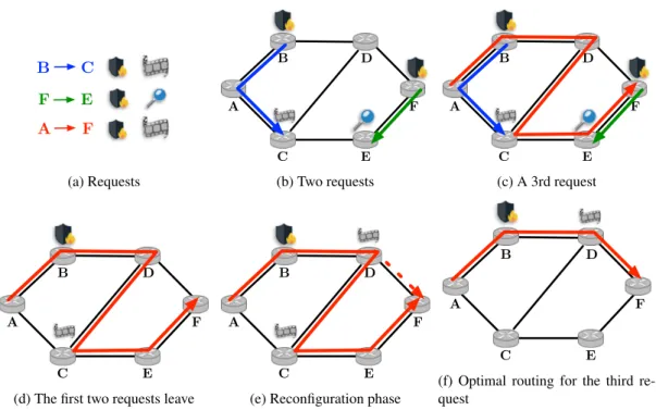
B C F E A F xx xx (a) Requests A B D F C E (b) Two requests A B D F C E (c) A 3rd request A B D F C E

(d) The first two requests leave

A

B D

F

C E

(e) Reconfiguration phase

A

B D

F

C E

(f) Optimal routing for the third re-quest

Figure 1: An example of the reconfiguration of a request using the make-before-break procedure. An Example. Figure 1 illustrates an example for the reconfiguration of a request using a make-before-breakprocess. When the request from A to F arrives, two requests have already been routed (step (b)). To avoid the cost of installing new VNFs, the route from A to F with minimum cost is a long 5–hops route (step (c)). When requests from B to C and from F to C leave, the request is routed on a non-optimal path (step (d)) which uses more resources than necessary. We compute one optimal 3-hops path and reroute the request to it (step (f)) with an intermediate make-before-break step (step (e)) in which both routes co-exist.

4

Modeling

In the considered setting, demands arrive and leave the network. To route them, we consider them one by one, and find the route which minimizes the additional network operational cost to be paid. Indeed, in an SDN network, even if multiple flows arrive simultaneously, they will be processed one by one by the SDN controller [19]. We then reconfigure the network to improve the network operational cost when one of the following conditions holds:

• Periodically, after a given period of time;

• When the set of requests has changed significantly (after a given number of SFC arrivals and de-partures);

• When a request arrives and cannot be accepted with the current provisioning and routing solution. The solution we propose, called Break-Free (for Break-Free Reconfiguration algorithm), imple-ments a make-before-break mechanism to avoid the interruption of the flows. In our experiimple-ments, we compare its results with a reconfiguration algorithm which does not implement such a mechanism, called Breaking-Bad(for Breaking-Bad Reconfiguration algorithm). This algorithm breaks the flows before

Layer 0 u1,0 u2,0 u3,0 Layer 1 u1,1 u2,1 u3,1 Layer 2 u1,2 u2,2 u3,2

Figure 2: The layered network GL(d) associated with a demand d such that vs = u1, vd = u3, and

cd= f1, f2, within a triangle network. f1is allowed be installed on u1and f2on u1and u3. Source and

destination nodes of GL(d) are u1,0and u3,2. Two possible SFCs that satisfy d are drawn in red (f1is in

u1, f2in u3) and blue (f1and f2is in u1).

rerouting them, and then packet loss occurred and QoS is degraded for these flows. When a reconfigura-tion has to be carried out, Breaking-Bad considers basically a static setting with the requests present in the network and finds an optimal Routing & Provisioning solution (R&P) without considering the current setting.

We present here three optimization models: (i) to solve the static problem (Section 4.2) used by Breaking-Bad, (ii) to route one demand when it arrives (Section 4.3), and (iii) to reconfigure the network with the make-before-break mechanism of Break-Free (Section 4.4).

Our models are based on the concept of a layered graph explained in a preliminary section (Sec-tion 4.1).

4.1

Layered graph

Similarly as in [20], in order to model the chaining constraint of a demand, we associate to each demand d a layered graph GL(d). We denote by ui,lthe copy of node uiin layer l. The path for demand d starts

from node vs,0in layer 0 and ends at node vd,|cd|in layer |cd| where |cd| denotes the number of VNFs in

the chain of the demand.

Given a link (ui, vj), each layer l has a link (ui,l, vj,l) defined. This property does not hold for links of

the kind (ui,l, ui,l+1). Indeed, a node may be enabled to run only a subset of the virtual functions. To

model this constraint, given a demand d we add a link (ui,l, ui,l+1) only if Node u is enabled to run the

(l + 1) − th function of the chain of d. The l − th function of the chain of d will be denoted by fcd

l .

A path on the layered graph corresponds to an assignment to a demand of both a path and the locations where functions are being run. Using a link (ui,l, vj,l) on GL, implies using link (u, v) on G. On the other

hand, using link (ui,l, ui,l+1) implies using the (l + 1) − th function of the chain at node u. Capacities

of both nodes and links are shared among layers.

4.2

Static R&P: Breaking-Bad

To solve the static R&P problem, we use an ILP given below. The ILP routes the demands by finding a path on the layered graph for each of them. In doing this, both node and link capacities must be respected

as they are shared among all the demands. The ILP has the minimization of the network operational cost (i.e., bandwidth cost and network function activation cost) as an objective. As network functions can be shared, the ILP will try to activate a small number of network functions. The parameter β ≥ 0 specified by the network administrator accounts for different scales over which the functions’ activation cost is put in relationship with the network bandwidth cost. β can be defined as the ratio between the cost of sending 1 TB of traffic on a link and the cost of installing a function which can handle 1 TB of data.

Model. The ILP takes as an input the set of demands D. The output corresponds to the minimum cost SFC-R&P.

Variables: • ϕd

uv,i≥ 0 is the amount of flow on Link (u, v) in Layer i for Demand d.

• αd

u,i≥ 0 is the fraction of flow of Demand d using Node u in Layer i.

• zu,f ∈ {0, 1}, where zu,f = 1 if function f is activated on Node u.

Objective: minimize the amount of network resources consumed.

min X d∈D X (u,v)∈E |cd| X i=0 bwd· ϕduv,i+ β · X u∈V X f ∈F cu,f · zu,f

Flow conservation constraints. For each Demand d ∈ D, Node u ∈ V . X (u,v)∈ω+_(u) ϕd_uv,0 − X (v,u)∈ω−_(u) ϕd_vu,0+ αd_u,0= ( 1 if u = vs 0 else (1) X (u,v)∈ω+(v) ϕd_uv,|cd| − X (v,u)∈ω−_(v) ϕd_vu,|cd|− αd u,|cd|−1= ( −1 if v = vd 0 else (2) X (u,v)∈ω+_(u) ϕd_uv,i − X (v,u)∈ω−_(u) ϕd_vu,i+ αd_u,i−1− αd u,i−1= 0.(0 < i < |cd|) (3)

Node capacity constraints. The capacity of a node u in V is shared between each layer and cannot exceed Cu. For each Node u ∈ V .

X d∈D bwd |cd|−1 X i=0 ∆_fcd i · α d u,i≤ Cu. (4)

Link capacity constraints. The capacity of a link (u, v) ∈ E is shared between each layer and cannot exceed Cuv. For each Link (u, v) ∈ E.

X d∈D bwd |cd| X i=0 ϕd_uv,i≤ Cuv. (5)

Functions activation. To know which functions are activated on which nodes. For each Node u ∈ V , Function f ∈ F , Demand d ∈ D, Layer i ∈ {0, ..., |cd| − 1}.

αd_u,i≤ z_u,fcd

i (6)

Location constraints. A node may be enabled to run only a subset of the virtual network functions. For each Demand d ∈ D, Node u ∈ V , layer i ∈ {0, ..., |cd| − 1}, if the (i + 1) − th function of cdcannot

be installed on Node u, we add the following constraint.

4.3

R&P for a single demand

Note first, that even routing a single demand is NP-hard as it is equivalent to find a shortest Weight-Constrained Path [21] in the layered graph as link and node capacities are shared between layers [20]. A solution is to use the ILP for static R&P in which all the demands routed in the past are fixed. The ILP routes the demand (if possible) with the goal of minimizing the additional needed cost without exceeding the available network resources. To deal with the already installed network function, the current cost ˜cu,f

of installing a network function f on a Node u is defined as follows. Let I be the set with the already installed network function, then ˜cu,f = 0 if (u, f ) ∈ I, and cu,f otherwise.

Model.The ILP takes as an input a demand d = (vs, vd, cd, bwd) and the network. We denote by Ruthe

residual capacity of a Node u, and finally by Ruvthe residual capacity of a link (u, v).

Variables:

• ϕuv,i≥ 0 is the amount of flow on Link (u, v) in Layer i.

• αu,i≥ 0 is the fraction of flow of the demand using Node u in Layer i at time step t.

Objective: minimize the additional increase in terms of network operational cost.

min X (u,v)∈E |cd| X i=0 bwd· ϕuv,i+ β · X u∈V |cd|−1 X i=0 ˜ c_u,fcd i · αu,i

Flow conservation constraints. For each Node u ∈ V . X (u,v)∈ω+_(u) ϕuv,0 − X (v,u)∈ω−_(u) ϕvu,0 + αu,0= ( 1 if u = vs 0 else (8) X (u,v)∈ω+_(v) ϕuv,|cd| − X (v,u)∈ω−_(v) ϕvu,|cd| − αu,|cd|−1= ( −1 if v = vd 0 else (9) X (u,v)∈ω+_(u) ϕuv,i − X (v,u)∈ω−_(u)

ϕvu,i+ αu,i−1− αu,i−1= 0.

0 < i < |cd| (10)

Node capacity constraints. The capacity of a node u in V is shared between each layer and cannot exceed the residual capacity Ru. For each Node u ∈ V .

bwd |cd|−1 X i=0 ∆_fcd i · αu,i≤ Ru. (11)

Link capacity constraints. The capacity of a link (u, v) ∈ E is shared between each layer and cannot exceed the residual capacity Ruv. For each Link (u, v) ∈ E.

bwd |cd|

X

i=0

ϕuv,i ≤ Ruv. (12)

Another possibility is to adapt the pseudo-polynomial algorithms proposed for the shortest Weight-Constrained Path problem such as the Label-setting algorithm based on dynamic programming [22].

4.4

Break-Free

Reconfiguration (Make-before-break)

A first way to perform the reconfiguration at a given time t is to try to reconfigure to optimal. This is done in two phases. In the first one, we compute a minimum cost routing for the set of demands present at time t. This can be done by using the model for static R&P. In the second one, we compute the transitions from the current routing to the optimal routing for each demand, taking into account the intermediate make-before-break steps during which two paths co-exist for a demand which is changing its route. This can be done using the ILP presented in this section, taking as inputs the current and the minimum cost solutions.

However, the transitions to an optimal solution may be long to compute or even impossible to carry out. Indeed, in complex scenarios (which occur when the network is saturated), the transition to the new routes cannot be performed directly. This is mainly due to two reasons.

First, in an intermediate step of the reconfiguration, two routes are provided, leading to an increased use of the network resources. Second, a request may have to be moved in an intermediate routing before being able to be moved to its final one in order to make place for the new routing of the first request. This needs to be done during distinct reconfigurations steps. Because of this, several intermediate steps of reconfigurations may be necessary, and each additional step of reconfiguration significantly increases the number of variables and constraints of the problem, and thus the time needed to obtain an optimal solution. Therefore, we propose a best effort reconfiguration.

Best Effort Reconfiguration. The idea here consists in improving the R&P as much as possible instead of setting a final R&P as a target. To this end, we set a number of intermediate reconfiguration steps, T , (how to set T is discussed below) and the goal of the optimization is to find a routing with minimal cost which can be reached from the current routing using T reconfiguration steps. Note that the best effort reconfiguration has several advantages compared to the reconfiguration to optimal. It will give a solution as good as the reconfiguration to optimal when such a reconfiguration is possible. Indeed, several optimal solutions may exist, and only part of them could be reached using reconfiguration. Reconfiguration to optimal is focusing on only one, when Best Effort reconfiguration could reach any of those. Second, when reconfiguration to optimal is not possible, Best Effort reconfiguration may still be able to find a solution better than the current one. This is why we used Best Effort reconfiguration in our experiments. Best Effort reconfiguration can be modeled using the ILP presented in the following. At time 0, the R&P is set to the current one. Then, at each step of reconfiguration, a set of demands can be rerouted as long as there are enough link and node capacities to satisfy the intermediate make-before-break reconfig-uration steps. This can be modeled linearly by defining a variable which is equal to 1 if a resource is used by a request either at time t − 1 or at time t. As a single step of reconfiguration may not be enough, the ILP has several intermediate reconfiguration steps, each corresponding to a solution of the R&P problem. The objective function is to minimize the cost of the R&P of the final state.

Note that reconfiguration to optimal can be modeled using the same ILP with a few changes. We just have to set the variables corresponding to the final state to the minimum cost R&P computed previously. Choosing T , the number of reconfiguration steps. The value of T is an important parameter. Indeed, a value too small may lead to models with no solution, while a value too large to models with prohibitive execution times. This is why we tested different values in our experiments. We observe that when the network is not congested, corresponding to the low-traffic scenarios of Section 5.2, a single reconfigura-tion step is enough to provide optimal (or close to optimal) solureconfigura-tions while it leads to solureconfigura-tions almost as bad as without reconfiguration in the high-traffic scenarios of Section 5.3. In the later scenarios, at least 2 reconfiguration steps are necessary. A good way to find the right value is to start with T = 1, which is the fastest model, and then to increase progressively the value of T until either the solution does not improve any more or the model solving time is too long. Note that, when a maximum solving time is set, the largest possible value of T leading to a lower solving time can also be found by dichotomy.

Model. The ILP takes as an input both the current configuration (i.e., paths and function locations for all the demands) and the number of time steps T to be used in the reconfiguration process. The output corresponds to both the final SFC-R&P at time T after the reconfiguration process and the intermediate SFC-R&P to be used to reach the final state. Between two consecutive time steps t0< ... < ti< ti+1 <

... < T , a subset of the demands may be moved to a new route. In doing this, resources of both nodes and links must not be exceeded in order to not interrupt connections (make-before-break).

Variables:

• ϕd,t_uv,i≥ 0 is the amount of flow on Link (u, v) in Layer i at time step t for Demand d. • αd,t_u,i≥ 0 is the fraction of flow of Demand d using Node u in Layer i at time step t.

• xd,t_uv,i≥ 0 is the maximum amount of flow on Link (u, v) in Layer i at time steps t and t − 1 for Demand d.

• y_u,id,t≥ 0 is the maximum fraction of flow of demand d using Node u in Layer i at time steps t or t − 1. • zT

u,f ∈ {0, 1}, where z f

u= 1 if function f is activated on Node u at time step T in the final routing.

The optimization model starts with the initial configuration as an input. Thus, for each demand d ∈ D the variables ϕd,0_uv,i (for each node u ∈ V , layer i ∈ {0, ..., |cd|}) and αd,0u,i (for each link (u, v) ∈ E,

layer i ∈ {0, ..., |cd|}) are known. The ILP is based on the layered graph described in Section 4.1 and it

is written as follows.

Objective: minimize the amount of network resources consumed during the last reconfiguration time step T . min X d∈D X (u,v)∈E |cd| X i=0 bwd· ϕd,Tuv,i+ β · X u∈V X f ∈F cu,f · zu,fT

Flow conservation constraints. For each Demand d ∈ D, Node u ∈ V , time step t ∈ {1, ..., T }.

X (u,v)∈ω+_(u) ϕd,t_uv,0 − X (v,u)∈ω−_(u) ϕd,t_vu,0 + αd,t_u,0= ( 1 if u = vs 0 else (13) X (u,v)∈ω+_(v) ϕd,t_uv,|c d| − X (v,u)∈ω−_(v) ϕd,t_vu,|c d| − αd,t_u,|c d|−1= ( −1 if v = vd 0 else (14) X (u,v)∈ω+_(u) ϕd,t_uv,i − X (v,u)∈ω−_(u)

ϕd,t_vu,i+ αd,t_u,i−1− αd,t_u,i−1= 0.

0 < i < |cd| (15)

Node usage over two consecutives time periods. For each Demand d ∈ D, Node u ∈ V , Layer i ∈ {0, ..., |cd| − 1} time step t ∈ {1, ..., T }.

αd,t_u,i≤ yd,t_u,iand αd,t−1_u,i ≤ yd,t_u,i αd,t_u,i+ αd,t−1_u,i ≥ yd,t_u,i

i ∈ {0, ..., |cd|} time step t ∈ {1, ..., T }.

ϕd,t_uv,i≤ xd,t_uv,iand ϕd,t−1_uv,i ≤ xd,t_uv,i ϕd,t_uv,i+ ϕd,t−1_uv,i ≥ xd,t_uv,i

Make Before Break - Node capacity constraints. The capacity of a node u in V is shared between each layer and cannot exceed Cuconsidering the resources used over two consecutives time periods. For each

Node u ∈ V , time step t ∈ {1, ..., T }. X d∈D bwd |cd|−1 X i=0 ∆_fcd i · y d,t u,i≤ Cu. (16)

Make Before Break - Link capacity constraints. The capacity of a link (u, v) ∈ E is shared between each layer and cannot exceed Cuvconsidering the resorces used over two consecutives time periods. For each

Link (u, v) ∈ E, time step t ∈ {1, ..., T }. X d∈D bwd |cd| X i=0 xd,t_uv,i≤ Cuv. (17)

Location constraints. A node may be enabled to run only a subset of the virtual network functions. For each Demand d ∈ D, Node u ∈ V , layer i ∈ {0, ..., |cd| − 1}, if the (i + 1) − th function of cdcannot

be installed on Node u, we add the following constraint for each time step t ∈ {1, ..., T }.

αd,t_u,i= 0 (18)

Functions activation. To know which functions are activated on which nodes in the final routing. For each Node u ∈ V , Function f ∈ F , Demand d ∈ D, and Layer i ∈ {0, ..., |cd| − 1},

αd,T_u,i ≤ zT

u,f_icd. (19)

Note that we do not consider the cost of potential activations of VNFs during the reconfiguration process. Indeed, our goal is to minimize the network operational cost over time and the reconfiguration duration is very small in comparison in an SDN network [23].

5

Numerical Results

In this section, we evaluate the performance of our proposed solution, Break-Free. We study the impact of the reconfiguration on different metrics such as cost savings, acceptance rate, and resource usage. We first present the data sets we use for the experiments. Then, we compare the results with the ones of Breaking-Bad, which computes an optimal R&P for the whole set of requests (ILP of Section 4.2) for each SFC arrival and with No-Reconf which computes the R&P problem for a single demand, the newly arrived SFC (Section 4.3).

We consider two scenarios, one with low traffic in which basically all demands can be accepted and one with high traffic in which some have to be rejected. In the low traffic scenario, we can fairly compare resource usage using the different algorithms Break-Free, Breaking-Bad, and No-Reconf, as they are accepting the same demands. In the high traffic scenarios, we can compare them in terms of acceptance rate of demands.

We show in particular that Break-Free allows to lower the network cost and increase the acceptance rate almost as much as Breaking-Bad. For both algorithms, a large number of demands have to be rerouted, showing that it is crucial to implement a mechanism to avoid an impact on them. Network reconfiguration has to done often to attain a significant gain, however, this reconfiguration can be quickly computed. This makes reconfiguration feasible to be put into practice.

5.1

Data sets

We conduct experiments on two real-world topologies from SNDlib [24] of different sizes: pdh (11 nodes, 34 links), and ta1 (24 nodes, 55 links). We generate our problem instances as follows. We considered 250 demands for each network. The source and destination of each demand are chosen uni-formly at random among the nodes. Following [25], the lifetime of a demand is exponentially distributed with mean µ = 25. We then round this lifetime to an integral number of time steps. The volume of the demands is chosen randomly and is on average 2 times higher in the high-traffic scenario than in the low-traffic one. Also, each demand is associated with an ordered sequence of 2 to 3 functions uniformly chosen at random from a set of 5 different functions. Experiments have been conducted on an Intel Xeon E5520 with 24GB of RAM.

5.2

Low-traffic scenario - Resource usage

In Figure 5, we show the network cost for our low-traffic scenario. The results are given for No-Reconf and Breaking-Bad as a measure of comparison, and for several variants of Break-Free with dif-ferent numbers of reconfiguration steps from 1 to 4.

We first see that Break-Free has similar performances to Breaking-Bad, which interrupts the requests when moving them to an optimal state in terms of network operational cost. This means that our solution is as efficient as possible as Breaking-Bad provides a lower bound of the best our algorithm can achieve. Moreover, Break-Free achieves this performance for any number of time steps (even 1). This leads to a very fast algorithm as discussed below. This is due to the fact that when the network is not congested, there is enough capacity to host both the old and new routes.

Reconfiguration leads to a better resource utilization and reduces the network operational cost com-pared to No-Reconf, and this given a same volume of traffic (note that no demand is rejected in this scenario). Indeed, reconfiguring the network regularly permits a reduction of 19% of network operational cost while using 22.5% fewer VNFs and 18.5% less link bandwidth compared to the no-reconfiguration case. Results for bandwidth and VNF usages are given in Fig. 3, Fig. 4. Recall that the network cost is the result of the addition of the bandwidth and VNF costs.

5.3

High-Traffic scenario - Acceptance Rate

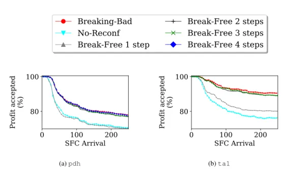
In our high-traffic scenario, the network is congested as there are not enough resources to satisfy all the demands. As a consequence, some requests cannot be accepted. We show, in Figure 6, the profit achieved by Break-Free, Breaking-Bad, and No-Reconf. We define the profit associated with an accepted demand as the asked volume of bandwidth multiplied by its duration.

The global profit is defined as the sum of all the accepted requests’ profits. We show the profit as a percentage in terms of maximum achievable profit. It can be seen that No-Reconf and Break-Free (with 1-step) lead to equivalent profit, around 70% for pdh (and between 78 and 81% for ta1), while Break-Free(with 2, 3, and 4 steps) and Breaking-Bad have similar performances (around 80% for pdhand 90% for ta1). For this congested scenario, one step of reconfiguration is not enough as there is not enough place to move the requests. Therefore, some requests are rejected. Allowing to use more steps in our make-before-break reconfiguration process, without interrupting the requests, we can reach the same performances as Breaking-Bad.

In Figure 7, we show the network operational cost for Break-Free, Breaking-Bad, and No-Reconf as a function of the number of demands arrived. The first observation is that Break-Free (with 2, 3, 4 steps) leads to a smaller network operational cost than No-Reconf. It accepts more, with less cost. The second observation is that even if Break-Free (with 1-step) has a similar profit to No-Reconf, it has substantially less network operational cost than all the other algorithms.

Breaking-Bad

No-Reconf

Break-Free 1 step

Break-Free 2 steps

Break-Free 3 steps

Break-Free 4 steps

0

50

100

150

SFC Arrival

0

25

50

VNFs deployed

(%)

0

50

100

150

SFC Arrival

0

20

40

VNFs deployed

(%)

Figure 3: Low-Traffic scenario - Number of VNFs deployed across time.

0

50

100

150

SFC Arrival

0

20

40

Link usage (%)

0

50

100

150

SFC Arrival

0

20

40

Link usage (%)

Figure 4: Low-Traffic scenario - Bandwidth usage across time.

0

50

100

150

SFC Arrival

600

800

Network cost

0

50

100

150

SFC Arrival

600

800

1000

Network cost

Figure 5: Low-Traffic scenario - Network cost.

5.4

Impact of Parameter β

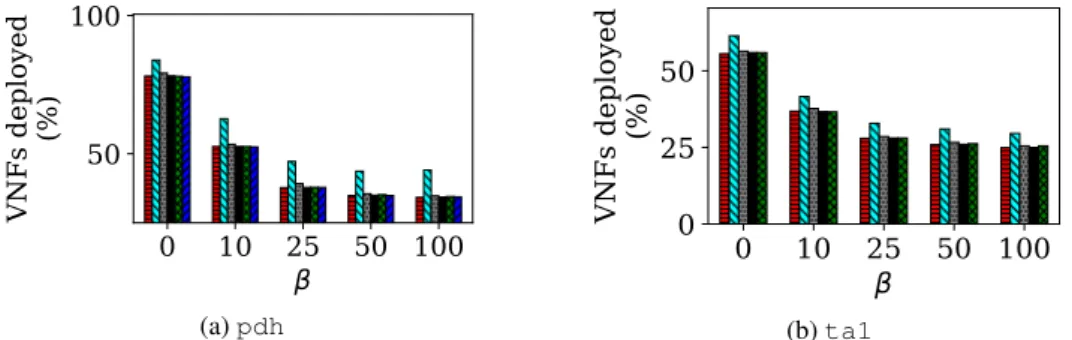
In Figures 8 and 9, we study the impact of the β parameter on the resources required in the network in terms of bandwidth and number of deployed VNFs, respectively. We focus on the low-traffic scenario as

Breaking-Bad

No-Reconf

Break-Free 1 step

Break-Free 2 steps

Break-Free 3 steps

Break-Free 4 steps

0

100

200

SFC Arrival

80

100

Profit accepted

(%)

0

100

200

SFC Arrival

80

100

Profit accepted

(%)

Figure 6: High-Traffic scenario - Percentage of accepted profit across time.

0

100

200

SFC Arrival

600

800

1000

Network cost

0

100

200

SFC Arrival

1000

1500

Network cost

Figure 7: High-Traffic scenario - Cost gain across time.

the compared algorithms accept the same requests and therefore, we can compare the utilisation of the network resources in terms of link bandwidth and number of VNFs deployed for the same global volume of traffic.

As β increases, the impact of the VNF cost on the total cost is greater. As a consequence, the number of deployed VNFs decreases, leading to longer routes and thus, to an increased amount of bandwidth necessary in the network to route the demands in order to satisfy their chaining constraints.

Note also that, for all values of beta, reconfiguration using Break-Free (for any number of steps) leads to similar gains to reconfiguration using Breaking-Bad. This shows that the conclusion dis-cussed in Section 5.2 for a specific value of β = 25 (our default value) is valid in more general settings for a wide range of β.

Another important observation is that the gain of reconfiguration is higher for larger values of β. The reason is that, when β is large, the requests tend to use longer routes as the cost of bandwidth is less important compared to the one of VNFs. This leads to requests routed in a very suboptimal way when other requests using the same VNFs leave (as shown in the example of Figure 1). On the contrary, when β is small, the routes try to always use close to shortest path solutions, leading to lower gains. There is still a gain as a shortest path is not always available (due to nodes and link capacities).

Breaking-Bad

No-Reconf

Break-Free 1 step

Break-Free 2 steps

Break-Free 3 steps

Break-Free 4 steps

0 10 25 50 100

0

20

40

Link usage (%)

0 10 25 50 100

0

20

40

Link usage (%)

Figure 8: Low-Traffic scenario - Impact of parameter β - Bandwidth usage as a function of β.

0 10 25 50 100

50

100

VNFs deployed

(%)

0 10 25 50 100

0

25

50

VNFs deployed

(%)

Figure 9: Low-Traffic scenario - Impact of parameter β - VNFs deployed as a function of β.

5.5

Time limits for the reconfiguration

Figure 10 shows the gains of network cost (compared to No-Reconf) in percentage for Break-Free (1 to 4 steps) and Breaking-Bad when limiting the time spent for the reconfiguration. Break-Free with 1 step needs only 1 second to reach its best solution. This variant of the algorithm is almost as fast as Breaking-Bad (which does not compute an intermediate make-before-break step). 10 seconds are needed to reach a close to optimal solution for the 2–step variant, and a good solution for the 3–step variant. The best solution is attained after 1 minute. We remind the reader that in the low-traffic scenario, the 1–step variant is enough to achieve solutions close to optimal, while in the high-traffic scenario, this is the case of the 2 step variant. It is thus possible to reconfigure a network with significant gain in a few seconds.

5.6

Reconfiguration Rate

In this experiment, we test different reconfiguration rates. Note that during the previous simulations, we reconfigured the network considering the three conditions defined in the beginning of Section 4. Here, the only condition to reconfigure is the first one, i.e., periodically, after a given number of time steps, defined as the reconfiguration rate.

0.1

1

10

60

Max reconf time (s)

0

10

20

Network cost reduction (%)

(a) Break-Free (1 step)

0.1

1

10

60

Max reconf time (s)

0

10

20

Network cost reduction (%)

(b) Break-Free (2 steps)

0.1

1

10

60

Max reconf time (s)

0

10

20

Network cost reduction (%)

(c) Break-Free (3 steps)

0.1

1

10

60

Max reconf time (s)

0

10

20

Network cost reduction (%)

(d) Breaking-Bad

Figure 10: Low-Traffic scenario - Gains of network operational costs for different time limits for the optimization process.

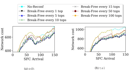
The faster rate is to reconfigure every time step, while the slowest one in our setting would be to reconfigure every 100 time steps (only 1 or 2 reconfigurations are performed during the whole test). We thus present the results for reconfiguration rates of every 1, 5, 10, 15, 50, and 100 time steps. In Figure 11, we provide the network cost in the low-traffic scenario. The minimum cost is as expected achieved when reconfiguring at each time step. However, in this setting similar gain can be obtained when reconfiguring every 10 and 15 time steps for pdh and ta1.

Results for the high-traffic scenarios can be seen in Figure 12, in which we report the profit generated by the accepted demands. In this setting, the network is congested. This means that very frequently the demand arriving at a time step cannot be routed directly. For pdh, not reconfiguring at every time step leads to poor performance, whatever the value of the reconfiguration rate. For ta1, this effect is not as stringent. Different reconfiguration rates lead to different values of profit. However, only a reconfiguration every time step leads to an optimal performance.

Thus, the reconfiguration should be well chosen by network operators, depending on their network usage. The higher the congestion, the higher the rate should be.

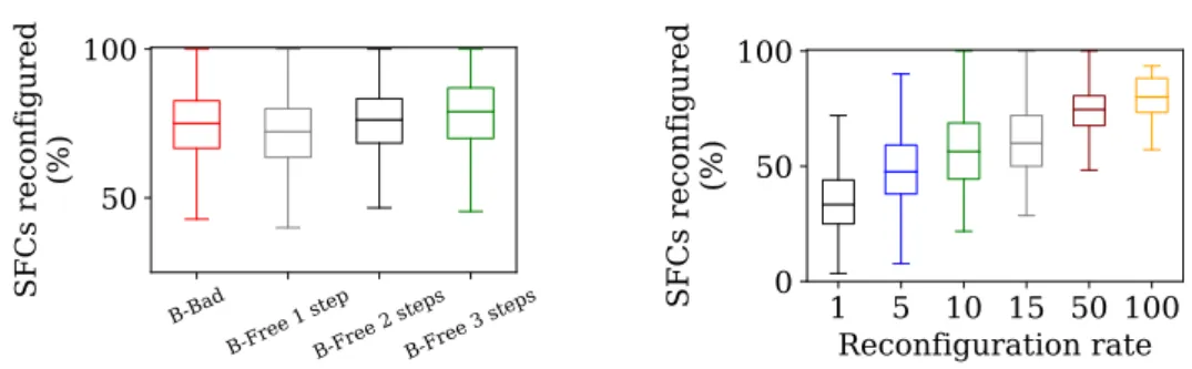
5.7

Percentage of rerouted requests

To see the importance of implementing a make-before-break process, we study the percentage of rerouted requests during the reconfiguration process. We report in Figure 13 (left) the percentage of reconfig-ured SFCs for Break-Free (1 to 4 steps) and Breaking-Bad for the high-traffic scenario. Firstly, Breaking-Badhas to interrupt, on average, 78% of the requests (between 45% and 100%) to maintain an optimal solution. This is thus of crucial importance to avoid impacting this large number of requests when reconfiguring.

No-Reconf

Break-Free every 1 top

Break-Free every 5 tops

Break-Free every 10 tops

Break-Free every 15 tops

Break-Free every 50 tops

Break-Free every 100 tops

0

50

100

150

SFC Arrival

400

600

Network cost

0

50

100

150

SFC Arrival

600

800

1000

Network cost

Figure 11: Low-Traffic scenario - impact of the reconfiguration rate on the network cost.

0

100

200

SFC Arrival

70

80

90

100

Profit accepted

(%)

0

100

200

SFC Arrival

70

80

90

100

Profit accepted

(%)

Figure 12: High-Traffic scenario - impact of the reconfiguration rate on the percentage of profit accepted.

Break-Freechanges the routing of approximately the same number of requests but without any inter-ruption of traffic. For the 1-step case, the reconfiguration is not always possible as the network is almost saturated. Therefore, when reconfiguration is achieved, it impacts slightly less requests: 65% on average for pdh and 70% for ta1.

Note that the number of reconfigured requests depends on the frequency of the reconfiguration, as shown in Figure 13 (right).

6

Conclusion

In this work, we provide a solution, Break-Free, to reconfigure a set of requests which have to go through service function chains. The requests are routed greedily when they arrive, leading to a sub-optimal use of network resources, bandwidth, and virtual network functions. Break-Free reroutes the requests to an optimal or close to optimal solution while providing a make-before-break mechanism to avoid impacting the rerouted requests.

Our algorithm is fast and provides a close to optimal reconfiguration in a few seconds. However, as a future work, we plan to propose algorithms to handle larger instances.

B-Bad

B-Free 1 stepB-Free 2 stepsB-Free 3 steps

50

100

SFCs reconfigured

(%)

1 5 10 15 50 100

Reconfiguration rate

0

50

100

SFCs reconfigured

(%)

Figure 13: Percentage of rerouted requests for ta1, considering (left) different intermediate reconfigura-tion steps and (right) different reconfigurareconfigura-tion rates.

References

[1] H. Kim and N. Feamster, “Improving network management with software defined networking,” IEEE Communications Magazine, 2013.

[2] J. Sherry, S. Hasan, C. Scott, A. Krishnamurthy, S. Ratnasamy, and V. Sekar, “Making middle-boxes someone else’s problem: network processing as a cloud service,” ACM SIGCOMM Computer Communication Review, vol. 42, no. 4, pp. 13–24, 2012.

[3] P. Quinn and T. Nadeau, “Problem statement for service function chaining,” Tech. Rep., 2015. [4] J. Matias, J. Garay, N. Toledo, J. Unzilla, and E. Jacob, “Toward an sdn-enabled nfv architecture,”

IEEE Communications Magazine, vol. 53, no. 4, pp. 187–193, 2015.

[5] I. Fajjari, N. Aitsaadi, G. Pujolle, and H. Zimmermann, “Vnr algorithm: A greedy approach for virtual networks reconfigurations,” in IEEE GLOBECOM, 2011.

[6] L. Gao and G. N. Rouskas, “Virtual network reconfiguration with load balancing and migration cost considerations,” in IEEE INFOCOM, 2018.

[7] P. N. Tran and A. Timm-Giel, “Reconfiguration of virtual network mapping considering service disruption,” in IEEE ICC, 2013.

[8] Z. Cai, F. Liu, N. Xiao, Q. Liu, and Z. Wang, “Virtual network embedding for evolving networks,” in IEEE GLOBECOM, 2010.

[9] J. G. Herrera and J. F. Botero, “Resource allocation in nfv: A comprehensive survey,” IEEE Trans-actions on Network and Service Management, vol. 13, no. 3, pp. 518–532, 2016.

[10] R. Mijumbi, J. Serrat, J.-L. Gorricho, N. Bouten, F. De Turck, and R. Boutaba, “Network function virtualization: State-of-the-art and research challenges,” IEEE Communications Surveys & Tutori-als, 2016.

[11] S. Paris, A. Destounis, L. Maggi, G. S. Paschos, and J. Leguay, “Controlling flow reconfigurations in sdn,” in IEEE INFOCOM, 2016.

[12] S. Ayoubi, Y. Zhang, and C. Assi, “A reliable embedding framework for elastic virtualized services in the cloud,” IEEE Transactions on Network and Service Management, vol. 13, no. 3, pp. 489–503, 2016.

[13] M. Ghaznavi, A. Khan, N. Shahriar, K. Alsubhi, R. Ahmed, and R. Boutaba, “Elastic virtual network function placement,” in Cloud Networking (CloudNet), 2015 IEEE 4th International Conference on. IEEE, 2015, pp. 255–260.

[14] V. Eramo, E. Miucci, M. Ammar, and F. G. Lavacca, “An approach for service function chain routing and virtual function network instance migration in network function virtualization architectures,” IEEE/ACM Transactions on Networking, vol. 25, no. 4, pp. 2008–2025, 2017.

[15] J. Liu, W. Lu, F. Zhou, P. Lu, and Z. Zhu, “On dynamic service function chain deployment and readjustment,” IEEE Transactions on Network and Service Management, vol. 14, no. 3, pp. 543– 553, 2017.

[16] B. Augustin, T. Friedman, and R. Teixeira, “Measuring load-balanced paths in the internet,” in Proceedings of the 7th ACM SIGCOMM conference on Internet measurement, 2007.

[17] N. Garg and J. Koenemann, “Faster and simpler algorithms for multicommodity flow and other fractional packing problems,” SIAM Journal on Computing, vol. 37, no. 2, pp. 630–652, 2007. [18] Y. Sang, B. Ji, G. R. Gupta, X. Du, and L. Ye, “Provably efficient algorithms for joint placement

and allocation of virtual network functions,” in IEEE INFOCOM, 2017.

[19] W. Ma, O. Sandoval, J. Beltran, D. Pan, and N. Pissinou, “Traffic aware placement of interdependent nfv middleboxes,” in IEEE INFOCOM, 2017.

[20] N. Huin, B. Jaumard, and F. Giroire, “Optimal network service chain provisioning,” IEEE/ACM Transactions on Networking, 2018.

[21] M. R. Garey and D. S. Johnson, Computers and intractability. wh freeman New York, 2002, vol. 29.

[22] S. Irnich and G. Desaulniers, “Shortest path problems with resource constraints,” in Column gener-ation. Springer, 2005, pp. 33–65.

[23] P. Berde, M. Gerola, J. Hart, Y. Higuchi, M. Kobayashi, T. Koide, B. Lantz, B. O’Connor, P. Ra-doslavov, W. Snow et al., “Onos: towards an open, distributed sdn os,” in Proceedings of the third workshop on Hot topics in software defined networking. ACM, 2014, pp. 1–6.

[24] S. Orlowski, R. Wess¨aly, M. Pi´oro, and A. Tomaszewski, “Sndlib 1.0—survivable network design library,” Wiley Networks, 2010.

[25] S. Sahhaf, W. Tavernier, M. Rost, S. Schmid, D. Colle, M. Pickavet, and P. Demeester, “Network service chaining with optimized network function embedding supporting service decompositions,” Computer Networks, vol. 93, pp. 492–505, 2015.

2004 route des Lucioles - BP 93 06902 Sophia Antipolis Cedex

Domaine de Voluceau - Rocquencourt BP 105 - 78153 Le Chesnay Cedex inria.fr