HAL Id: hal-02103880
https://hal.archives-ouvertes.fr/hal-02103880
Submitted on 18 Apr 2019
HAL is a multi-disciplinary open access archive for the deposit and dissemination of sci-entific research documents, whether they are pub-lished or not. The documents may come from teaching and research institutions in France or abroad, or from public or private research centers.
L’archive ouverte pluridisciplinaire HAL, est destinée au dépôt et à la diffusion de documents scientifiques de niveau recherche, publiés ou non, émanant des établissements d’enseignement et de recherche français ou étrangers, des laboratoires publics ou privés.
Distributed under a Creative Commons Attribution - NonCommercial - NoDerivatives| 4.0 International License
food demand
Fabienne Femenia
To cite this version:
Fabienne Femenia. A meta-analysis of the price and income elasticities of food demand. [University works] Inconnu. 2019, 78 p. �hal-02103880�
A meta-analysis of the price and income elasticities of
food demand
Fabienne FEMENIA
Working Paper SMART – LERECO N°19-03
April 2019
UMR INRA-Agrocampus Ouest SMART - LERECO
Les Working Papers SMART-LERECO ont pour vocation de diffuser les recherches conduites au sein des unités SMART et LERECO dans une forme préliminaire permettant la discussion et avant publication définitive. Selon les cas, il s'agit de travaux qui ont été acceptés ou ont déjà fait l'objet d'une présentation lors d'une conférence scientifique nationale ou internationale, qui ont été soumis pour publication dans une revue académique à comité de lecture, ou encore qui constituent un chapitre d'ouvrage académique. Bien que non revus par les pairs, chaque working paper a fait l'objet d'une relecture interne par un des scientifiques de SMART ou du LERECO et par l'un des deux éditeurs de la série. Les Working Papers SMART-LERECO n'engagent cependant que leurs auteurs.
The SMART-LERECO Working Papers are meant to promote discussion by disseminating the research of the SMART and LERECO members in a preliminary form and before their final publication. They may be papers which have been accepted or already presented in a national or international scientific conference, articles which have been submitted to a peer-reviewed academic journal, or chapters of an academic book. While not peer-reviewed, each of them has been read over by one of the scientists of SMART or LERECO and by one of the two editors of the series. However, the views expressed in the SMART-LERECO Working Papers are solely those of their authors.
1
A meta-analysis of the price and income elasticities of food demand
Fabienne FEMENIA
SMART-LERCO, AGROCAMPUS OUEST, INRA, 35000, Rennes, France
Acknowledgements:
This work has been partly financed by the International Food Policy Research Institute (IFPRI). The author is grateful to David Laborde for his advises on the preliminary steps of this work, to Laure Latruffe and two anonymous reviewers for their helpful comments on the paper and to Christine Mesquida for her careful review of the references included in the meta-analysis.
Corresponding author Fabienne Femenia
INRA, UMR SMART-LERECO 4 allée Adolphe Bobierre, CS 61103 35011 Rennes cedex, France
Email : fabienne.femenia@inra.fr
Téléphone / Phone: +33(0)2 23 48 56 10
Les Working Papers SMART-LERECO n’engagent que leurs auteurs.
2 A meta-analysis of the price and income elasticities of food demand
Abstract
Food demand elasticities are crucial parameters in the calibration of simulation models used to assess the impacts of political reforms or to analyse long-term projections, notably in agricultural sectors. Numerous estimates of these parameters are now available in the economic literature. The main objectives of this work are twofold: we seek first to identify general patterns characterizing the demand elasticities of food products and second to identify the main sources of heterogeneity between the elasticity estimates available in the literature. To achieve these objectives, we conduct a broad literature review of food demand elasticity estimates and perform a meta-regression analysis.
Our results reveal the important impacts of income levels on income and price elasticities both at the country (gross domestic product-GDP) and household levels: the higher the income is, the lower the level of elasticities. Food demand responses to changes in income and prices appear to follow different patterns depending on the global regions involved apart from any income level consideration. From a methodological viewpoint, the functional forms used to represent food demand are found to significantly affect elasticity estimates. This result sheds light on the importance of the specification of demand functions, and particularly of their flexibility, in simulation models.
Keywords: elasticities, estimation, food demand, meta-analysis JEL classification: Q11, Q18, D12, C13
3 Une méta-analyse des élasticités prix et revenu de la demande de biens alimentaires
Résumé
Les élasticités prix et revenu de la demande de biens alimentaires sont des paramètres cruciaux intervenant dans le calibrage des modèles de simulation qui sont utilisés pour évaluer l’impact de réformes politiques ou faire des projections de long terme, notamment en ce qui concerne dans les secteurs agricoles. De nombreuses valeurs estimées de ces paramètres sont aujourd’hui disponibles dans la littérature économique. Nos principaux objectifs ici sont, d’une part, de mettre en avant des éléments caractérisant de manière générale ces élasticités prix et revenu et, d’autre part, d’identifier les principales sources de variabilité de leurs valeurs estimées dans la littérature. Pour répondre à ce double objectif nous collectons dans la littérature un large ensemble d’élasticités estimées de demande de biens alimentaires que nous analysons ensuite à l’aide d’une méta-régression.
Nos résultats mettent en évidence un impact important du niveau de revenu, à la fois au niveau pays (produit intérieur brut-PIB) et au niveau ménage, sur les élasticités prix et revenu : plus le revenu est élevé, moins la demande de biens alimentaires est élastique. Il apparait également que les réponses de la demande aux variations de revenu et de prix diffèrent entre régions du monde indépendamment des différences de revenus pouvant exister entre ces régions. D’un point de vue méthodologique, nous trouvons que le choix de la forme fonctionnelle utilisée pour représenter la demande a un effet significatif sur les élasticités estimées. Ce résultat souligne l’importance de la spécification des fonctions de demande, en particulier de leur flexibilité, dans les modèles de simulation.
Mots-clés : élasticités, estimation, demande de biens alimentaires, méta-analyse
4 A meta-analysis of the price and income elasticities of food demand
1. Introduction
Simulation models, such as general or partial equilibrium models, are often used to analyse long-term projections to assess the effects of political reforms or to shed light on a variety of issues, notably in agricultural sectors. These models use a large number of behavioural parameters, among which food demand elasticities play a crucial role (see, e.g., Rude and Meilke (2004) and Carpentier et al. (2015)). Indeed, these parameters provide information on how consumers react to income and price changes and are likely to have considerable impacts on the simulation outcomes of projection and political reform scenarios for two main reasons. First, the current global economic situation will undoubtedly evolve dramatically in the forthcoming years even if economic policies remain unchanged. This is particularly true for some developing countries in which incomes are expected to keep growing for several years. Since the level of food consumption is a key element to be analysed for one who is interested in economic projections, the impacts of income growth on household demand for food products, which strongly depend on income elasticities, must be accounted for as accurately as possible in simulation models. Second, even if agricultural policy reforms do not have strong impacts on national income levels because agriculture generally represents a small proportion of Gross Domestic Product (GDP), these reforms can have considerable impacts on agricultural prices. Demand responses to price changes are thus of crucial importance when one wishes to simulate the effects of agricultural policy reforms, and this depends on the value of food price elasticities. Numerous price and income elasticity estimates are available in the economic literature and can be used to calibrate large-scale simulation models. However, the studies from which these estimates can be drawn use different types of data, rely on various assumptions regarding the modelling of household food demand and use different econometric estimation methods. All these sources of heterogeneity among studies may lead to significant variations in the empirical estimates reported in the literature even if these estimates are supposed to measure the same phenomenon, the responses of food demand to income or prices.
Our main objective in the present study is to investigate this issue by performing a meta-analysis to identify and quantify the main sources of heterogeneity among the demand elasticity estimates available in the literature.
5
As emphasized by Nelson and Kennedy (2009), meta-analyses have been extensively used over the past decades in several areas, including economics, to synthetize information provided by empirical studies. Some meta-analyses of food demand elasticities have been conducted with the stated objective of revealing “true” values of these parameters. Green et al. (2013) and Cornelsen et al. (2016) notably conduct meta-analyses of own price and cross price elasticities for various food products to provide estimates of these parameters by country income group. Chen et al. (2016) also use a meta-analysis with the aim of providing estimates of price and income elasticities of food demand in China. Our objective here is slightly different: we seek to understand the heterogeneity of elasticity estimates across studies to help economists to select empirical estimates of these key parameters for their simulation models. We aim at identifying the key methodological aspects of primary studies that can have an impact on the values of elasticity estimates beyond the factual elements that may affect elasticity values, such as the type of food product or the country concerned. Our work also differs from Green et al. (2013) and Cornelsen et al. (2016) by focusing not only on prices but also on income elasticities, which, as explained above, can play a crucial role in long run projections and policy simulations. Furthermore, compared to these two studies, additional variables characterizing elasticity estimates are included in our analysis. We notably consider a more detailed categorization of functional forms representing food demand, household income level, and information necessary to assess publication bias, which is a pervasive issue among meta-analyses. Other meta-analyses have been conducted to examine heterogeneity in these food demand elasticities estimates with the aim of providing guidance on the study attributes to which attention should be paid. These studies generally focus only on the type of product, such as alcohol (e.g., Fogarty, 2010; Nelson 2013a and 2013b; Sornpaisarn et al., 2013; Wagenaar et al., 2009) or meat (Gallet 2008 and 2010). Santeramo and Shabnam (2015), Melo et al. (2015), Ogundari and Abdulai (2013) and Andreyeva et al. (2010) are exceptions since they consider various food products. However, Santeramo and Shabnam (2015), Melo et al. (2015) and Ogundari and Abdulai (2013) do not explicitly consider demand elasticities of food products but calorie- and/or nutrient-income elasticities. The analysis conducted by Andreyeva et al. (2010) is essentially descriptive and illustrates the potential heterogeneities that can exist between price elasticities estimates without seeking to precisely identify the sources of such heterogeneity. We go deeper here by relying on a meta-regression analysis (MRA) (Stanley and Jarell, 1989; Roberts, 2005). We also pay particular attention to conforming to the meta-analysis guidelines provided by the Meta-Analysis of Economics Research Network (MAER-NET) (Stanley et al., 2013), which
6
defines key issues related to data searches and coding and modelling strategies, that must be addressed in studies applying MRA to economics.
The next section is devoted to the description of the database of food demand elasticity estimates that we build to fulfil our objectives. In the third section, a descriptive analysis is presented to highlight several patterns characterizing own price and income elasticities in our database and to identify potential sources of heterogeneity among elasticity estimates. These sources are then statistically tested and quantified through an MRA in the fouth section, and conclusions are drawn in the last section.
2. Data search and coding methods
In line with the MAER-NET protocol, we provide here a detailed description of how the literature was searched and coded to build our database of price and income elasticity estimates. The procedure used to collect the references included in the database is presented first. A second part is devoted to the coding of information collected from primary studies. Finally, the selection of the sample used in the meta-analysis is described in a third part.
2.1 Data collection
Diverse data sources are commonly used to calibrate demand functions in global economic models (see, for instance, Valin et al. (2014) for a summary of data sources used in ten computable general equilibrium and partial equilibrium models). Several models, such as GCAM (Clarke et al., 2007), GLOBIOM (Havlik et al., 2011) and Mirage-BioF (Laborde and Valin, 2012), use the price elasticities provided in two reports released by the United States Department of Agriculture (USDA) (Seale et al. (2003a) and Muhammad et al. (2011)1) to calibrate their demand function parameters. In these reports, price and income elasticities are estimated for eight broad food categories (beverages and tobacco, bread and cereals, meat, fish, dairy products, oils and fats, fruits and vegetables and other food products) and for a large number of countries; own price and income elasticities are estimated for 114 countries in Seale
et al. (2003a) and for 144 countries in Muhammad et al. (2011). This broad level of country
coverage renders these elasticity data well-suited for calibrating large simulation models. Economists might however wish to use other source of elasticities for different reasons when, for instance, they consider food products at a higher disaggregation level or when they wish to
1 Muhammad et al. (2011) is an updated version of Seale et al. (2003a) considering more recent data and more
7
compare results obtained with a calibration of demand parameters based on USDA estimates to those obtained with a calibration based on other estimates given in the literature. The USDA provides a literature review database (USDA, 2005), which contains this type of information and is notably used to calibrate the IMPACT model (Robinson et al., 2015). This database collects own price, cross price, expenditure and income demand elasticity estimates from papers that have been published and/or presented in the United States (US) between 1979 and 2005. This represents a total of 1,800 estimates of own price and income elasticities collected from 72 papers. While the database covers a large variety of products at various aggregation levels2, few countries are included. The US is well-represented, with 1,166 elasticity estimates collected from 44 papers, which is not surprising given the focus of the database on papers published or presented in this country. The other elasticities are essentially for China with 528 estimates collected from 22 papers, and only four other countries (Canada, Indonesia, Portugal and Saudi Arabia) are represented, with a few estimates collected from up to three papers.
These two data sources, namely, the USDA’s estimates given in Seale et al. (2003a) and Muhammad et al. (2011) and the USDA’s literature review database, were used to build the database employed to conduct the meta-analysis presented here. More precisely, we started with the structure of the USDA literature review database, which already includes useful information on each elasticity estimate, such as the references of the papers from which the estimates have been collected; the countries, products and time periods concerned; the types of data used to conduct estimations; and the demand models estimated. The elasticities estimated by Seale et
al. (2003a) (1,824 estimates) and Muhammad et al. (2011) (2,304 estimates) were also included.
We then reviewed the primary studies to check the information included in the USDA database and to ensure the consistency of the data. Of the 74 references present in these data, five PhD dissertations were not available to us, thus restricting our ability to verify the data and to collect new information, and we decided to exclude these references.
Then, to broaden the scope of the data, we searched for new references providing food demand elasticity estimates in the economic literature with a focus on pre-2005 studies dealing with countries other than the US and China and with a focus on post-2005 studies regardless of country.
The search was performed with Google Scholar in March 2015 using the following combinations of keywords: “price, elasticities, food, demand” and “income, elasticities, food,
2 Product aggregation levels vary from global food aggregate (e.g., Han et al., 1997) to very detailed levels (e.g.,
8
demand”. We did not limit our search to published papers; working papers, reports, and papers presented at conferences were also included. A total of 72 references were collected in this way. All price and income elasticity estimates of food demand reported in these references were collected. Among own price elasticities we distinguished uncompensated (Marshallian) price elasticities from compensated (Hicksian) elasticities. This distinction is important since both elasticities do not measure the same type of demand response to prices: uncompensated elasticities measure the impact of a change in the price of one good by holding income and the prices of other goods constant, and they thus incorporate both income (when the price of one good increases, the income available to consume other goods decreases) and substitution effects (when the price of one good increases, other goods become relatively less expensive); compensated elasticities measure the impacts of a change in the price of one good holding consumer utility constant, i.e., they assume that price changes are compensated by income changes to maintain consumers’ utility levels and do not incorporate income effects. The two types of price elasticities can thus not be considered equivalent or be studied simultaneously. Given the small number of compensated own price elasticity estimates present in the USDA literature review database and reported in the references that we collected (680 of 5,968 own price elasticity estimates), we decided to focus on uncompensated price elasticities alone. Our final database includes 3,334 own price elasticities and 3,311 income elasticity estimates collected from 93 primary studies published between 1973 and 2014. Among these studies, a significant number of papers, such as Seale et al. (2003a) and Muhammad et al. (2011), are designed to provide estimates of food demand elasticities for subsequent use to understand the structure of demand for food products or to simulate the evolution of such demand under various scenarios. While Seale et al. (2003a) and Muhammad et al. (2011) include a large number of countries, most of these papers focus on one particular country and provide estimates for a complete set of food products or for one particular food sector, such as meat, dairy products or fruits and vegetables. In other primary studies, food demand elasticities are estimated to address specific empirical issues, such as the impacts of advertising, product differentiation, health policies or structural changes, on the structure of food demand. Finally, several demand elasticity estimates have been collected from primary studies that focused on methodological aspects, such as the functional forms of demand models or the estimation procedures used to estimate these models. In this case, elasticities are generally estimated for illustrative purposes to assess the proposed approach.
9 2.2 Information included and data coding
Based on the information collected during the review process, our database includes several variables in addition to the values of elasticity estimates and the references of the primary studies from which they have been collected3.
A first set of information included in our database relates to the primary data that have been used to estimate the demand elasticities. Information relates to the type of data used (time series, panel or cross section), to whether they have been collected at the micro (household) or macro (country) level, to the decade in which they have been collected, which ranges from 1950 to 2010, and to the countries and products to which these data refer. To homogenize the information on food products, product names as they appear in the primary studies are mapped to the following eight product categories: beverages and tobacco, cereals, dairy products, fruits and vegetables, oils and fats, meat and fish, other food products and non-food products. Given that these categories are in some cases much broader than the product levels considered in primary studies, a variable representing the aggregation level of the primary data is also associated with each observation. The following four aggregation levels are considered: “global food aggregate”; “product category aggregate”, which corresponds to the aforementioned categories; “product level”, which refers to single products, for instance bananas and apples for fruits, beef and poultry for meat, wheat and corn for cereals, etc.; “differentiated product level”, which refers to products differentiated by specific characteristics, for instance, organic or conventional for fruits and vegetables or cereals and types of cut for meat. Our mapping of product names, product categories and aggregation levels is presented in Appendix 2. Country names are converted into standard ISO-alpha-3 country codes (International Organization for Standardization) and are mapped to 11 world regions according to the classification provided in Appendix 3. Where applicable, we also report in our data information concerning the types (urban, rural or any type) and levels of income of households from which the primary data have been collected. While we also could have considered simple averages of elasticities for primary studies reporting estimates for different household categories, as in Cornelsen et al. (2015), this would have led to a loss of potentially important information. The levels of household income are homogenized across studies by reporting these levels as a percentage of the highest income considered in the study rather than as nominal income amounts.
3 Available human and financial resources did not allow for the data to be checked by an independent reviewer
as recommended under the MAER-NET protocol. An additional check was however performed by the author herself to limit potential data coding errors.
10
The second type of information included in the database relates to the precision of the elasticity estimates. This information is indeed necessary for assessing an important issue of meta-analysis, which is publication selection bias. Stanley (2005) identifies three sources of publication bias as follows: (i) papers are more likely to be accepted for publication when they conform to conventional views; (ii) when different models and/or estimation methods are tested, authors are more likely to report results corresponding to conventional views; and (iii) statistically significant results are treated more favourably. Hence, authors, reviewers and journal editors may have a preference for statistically significant results in line with conventional views, which results in studies finding small or insignificant estimates or estimates with unexpected signs to remain unpublished. In our case, publication bias may lead food demand elasticities to appear much larger in absolute terms than they actually are. It is thus necessary as a first step in our meta-analysis to test for the presence of a publication selection bias in our data. This can be accomplished by relying on a method proposed by Egger et al. (1997), the PET test (precision effect test), which involves regressing effect size estimates (demand elasticity estimates in our case) on an inverse indicator of their precision. This method allows one to test both for the presence of a publication bias and for the existence of a “true” effect size. Egger et al. (1997) suggest using the inverse standard errors of effect size estimates as indicators of their precision and thus regressing effect sizes on standard errors of estimates. When publication bias is detected, it must be accounted for in the subsequent meta-regression analysis. Stanley and Doucouliagos (2014) recommend that the PEESE (precision effect estimate with standard error) estimator be used in such cases, i.e., including the variances of effect size estimates as explanatory variables in the meta-regression. This approach thus also involves collecting information on the standard errors corresponding to each effect size (demand elasticities in our case) estimates from the primary studies. Unfortunately, we face here the same issue as that faced by other meta-analyses of demand elasticities: while studies generally report standard errors of primary estimates (estimates of demand model parameters), few report these elements for the elasticities that are computed from these estimates. In our sample, less than 30% of estimated elasticities have associated standard error estimates and/or Student’s t-test statistics, and we do not generally have sufficient information (complete covariance matrix of estimates) to use delta methods to compute standard error elasticity estimates. One solution involves only selecting studies with standard errors. This approach was adopted by Ogundari and Abdulai (2013) in their study of calorie-income elasticities and by Fogarty (2010) in his paper on alcohol demand elasticities. However, in our case, this would have substantially reduced the sample size and thus limited the possibility of conducting an
11
MRA. Some authors (Green et al., 2013; Cornelsen et al., 2015) do not treat publication bias because of this lack of standard error data. To avoid this issue we use inverse sample sizes or degrees of freedom (DF) instead of standard errors. Day (1999), among others, indeed demonstrates the link between sample sizes and standard deviations of estimates, and Egger et
al. (1997) recommend the use of sample size or DF as a measure of precision in the absence of
standard error estimates. These two pieces of information are thus collected and added to our database.
The last set of information included in our dataset relates to methodological aspects of elasticities estimations. We collected here all relevant information that could potentially help to explain the heterogeneity among elasticity estimates. This information essentially concerns the following econometric and modelling strategies adopted in primary studies: the functional form of the demand system from which elasticities are estimated; reliance on a multi-stage budgeting structure; the way in which zero values are treated in the estimation process; the use of unit values or quality adjusted prices; the inclusion of control variables related to household characteristics, product characteristics or time periods; and the econometric method used to estimate the demand model.
2.3 Sample selection
This subsection presents the selection procedure applied to the data sample used for the meta-analysis.
A first round of data selection was conducted based on the aggregation level of food products considered in the data used in the primary studies. Two of the four product aggregation levels identified in our dataset were excluded from the analysis as follows: the “global food aggregate” level and the “differentiated product” level, which includes very specific products that are of little relevance for large simulation models and for which elasticity estimates tend to be extremely high in absolute terms. This selection approach led to us exclude 42 primary studies and 1,959 elasticity estimates.
Then, we excluded primary studies that did not provide the number of observations used to estimate the elasticities since, as previously mentioned, this information is used as a proxy for the precision of elasticity estimates in the MRA. This selection approach led us to exclude 5 primary studies and 372 elasticity estimates.
12
We do not consider in our analysis the “non-food” and “beverage and tobacco” product categories, which correspond to 809 elasticity estimates. The “non-food” category indeed falls outside of the scope of our study and the demand for “beverage and tobacco” exhibits very specific patterns, which explains why a large number of meta-analyses have already been conducted on these products specifically.
Finally, as in Cornelsen et al. (2015), we consider as outliers price and income elasticities ranging outside of three standard deviations of their respective averages and exclude such outliers from our sample. This represents 63 observations for price elasticities and 41 observations for income elasticities.
The sample of elasticity estimates considered the paper thus includes 6,645 observations collected from 93 primary studies, among which 3,334 are price elasticities and 3,311 are income elasticities.
2. Descriptive analysis of the data
After discussing how price and income demand elasticities may differ across product categories and world regions, this section highlights other potential sources of heterogeneity among estimates related to the methodological approaches adopted in the primary studies.
2.1 Heterogeneity of elasticity estimates across food products
Table 1 reports, by product category and aggregation level sub-categories, the number of observations, weighted averages and standard deviations of price and income elasticities. More weight is given to more precise estimates in the computation of averages and standard deviations.
Table 1: Elasticities - summary statistics by food product categories
Own Price elasticities Income elasticities Nb Obs. Weighted Average Weighted S.D. Nb Obs. Weighted Average Weighted S.D. Fruits and vegetables
All 668 -0.61 0.69 694 0.61 0.68
Fruits and vegetables aggregate 327 -0.50 0.47 308 0.53 0.43
Product level 341 -0.71 0.79 386 0.67 0.81
Meat and fish
All 945 -0.57 0.53 946 0.73 0.66
Meat and fish aggregate 554 -0.50 1.09 579 0.67 0.43
13 Dairy products
All 419 -0.59 0.58 412 0.72 0.60
Dairy products aggregate 295 -0.57 0.38 283 0.70 0.43
Product level 124 -0.63 0.88 129 0.75 0.86
Cereals
All 520 -0.52 0.74 509 0.45 0.71
Cereals aggregate 306 -0.33 0.40 321 0.41 0.51
Product level 214 -0.72 0.85 188 0.50 0.95
Oils and fats
All 338 -0.44 0.56 326 0.46 0.56
Oils and fats aggregate 282 -0.36 0.40 269 0.38 0.33
Product level 56 -0.71 0.79 57 0.75 0.88
Other food products
All 444 -0.67 0.62 424 0.77 0.76
Other food products aggregate 307 -0.68 0.49 298 0.86 0.68
Product level 137 -0.66 0.84 126 0.58 0.81
Note: Primary studies sample sizes are used as weights to compute averages and standard deviations.
The products that are most well-represented in our database are meat and fish followed by fruits and vegetables, cereals, other food products, dairy products, and oils and fats.
From average elasticities computed over all product aggregation levels, the demand for cereals and oils and fats appears to be less responsive to price and income than the demand for meat and fish, dairy products and fruits and vegetables, which themselves are less responsive to price and income than the demand for other food products. This ranking of food products is not surprising since the consumption of staple products is generally less responsive to price and income changes than that of “luxury” foods (Tyers and Anderson, 1992). The same pattern appears for elasticities estimated at the aggregate product level, whereas the ranking is very different when we consider the elasticities estimated at the product level: the demand for oils and fats appears in this case to be, on average, the most responsive to price and income changes, while the demand for dairy products is the least responsive to price changes and the demand for other food products is the least responsive to income changes. The aggregation level of the data thus appears to have an impact on price elasticity estimates. It also appears in Table 1 that elasticities estimated on more disaggregated data (product level) tend to be higher in absolute terms than those estimated for broader product categories (aggregate product level). As mentioned by Eales and Unnevehr (1988), this might be attributed to substitution possibilities between disaggregated products, which reduce the average own price responses of product aggregates.
We can finally observe from Table 1 that the standard deviations in elasticity estimates are relatively high compared to the average values for each type of elasticity within each category of food product considered at a specific aggregation level. This suggests the presence of
14
additional sources of heterogeneity in elasticities, with one being location, as discussed in the following subsection.
2.2 Heterogeneity of elasticity estimates across regions
Consumption patterns can differ between countries for several reasons, including differences in tastes (see, e.g., Selvanathan and Selvanathan, 1993), implying variations in demand elasticities across countries. Table 2 reports the weighted averages and standard deviations of demand elasticity estimates for the 11 world regions and six product categories that we consider. We first note that again, standard deviations of elasticity estimates are relatively high compared to their average values and for the countries that are most well-represented in the database in particular, namely, North American, Asian and European Union (EU) countries.
15 Table 2. Elasticities - summary statistics by world regions
Own price elasticities Income elasticities
Cerea ls Dairy Fruit and veg. Meat Oils and Fat Other food Cerea ls Dairy Fruit and veg. Meat Oils and Fat Other food North America Weighted average -0.68 -0.41 -0.75 -0.62 -0.32 -0.41 0.68 0.52 0.69 0.71 0.48 0.62 Weighted S.D. 0.61 0.66 0.74 0.49 0.47 0.58 0.89 0.67 0.91 0.78 0.72 0.83 Nb Obs. 64 33 98 156 17 44 47 30 66 115 17 29 Latin America Weighted average -0.36 -0.58 -0.50 -0.54 -0.37 -0.61 0.42 0.84 0.62 0.74 0.49 0.72 Weighted S.D. 0.41 0.50 0.43 0.36 0.46 0.30 0.46 0.60 0.56 0.53 0.51 0.59 Nb Obs. 34 37 37 71 34 34 52 53 91 83 40 52 East Asia Weighted average -0.63 -0.69 -0.67 -0.66 -0.64 -0.64 0.55 0.71 0.73 0.82 0.66 0.77 Weighted S.D. 0.82 0.84 0.73 0.84 0.78 0.90 0.86 0.79 0.78 0.76 1.09 0.76 Nb Obs. 81 48 95 137 33 31 69 56 142 163 30 46 Asia Other Weighted average -0.59 -0.53 -0.64 -0.53 -0.59 -0.71 0.36 0.78 0.56 0.71 0.52 0.74 Weighted S.D. 0.86 0.55 0.79 0.54 0.52 0.66 0.82 0.68 0.79 0.77 0.51 0.86 Nb Obs. 122 70 157 121 47 92 116 57 134 126 35 74 European Union Weighted average -0.19 -0.55 -0.49 -0.49 -0.17 -0.53 0.25 0.64 0.45 0.69 0.22 0.61 Weighted S.D. 0.41 0.65 0.64 0.51 0.21 0.38 0.46 0.63 0.56 0.79 0.27 0.52 Nb Obs. 63 76 108 165 54 75 65 69 91 168 54 74 European Other Weighted average -0.42 -0.62 -0.70 -0.54 -0.42 -0.77 0.24 0.32 0.39 0.41 0.21 0.42 Weighted S.D. 0.66 0.56 0.86 0.62 0.60 0.75 0.33 0.19 0.23 0.18 0.22 0.43 Nb Obs. 12 12 12 18 12 12 12 12 12 18 12 12
16
Own price elasticities Income elasticities
Cerea ls Dairy Fruit and veg. Meat Oils and Fat Other food Cerea ls Dairy Fruit and veg. Meat Oils and Fat Other food Former Soviet Union Weighted average -0.32 -0.59 -0.43 -0.55 -0.34 -0.68 0.42 0.77 0.56 0.71 0.44 0.89 Weighted S.D. 0.16 0.14 0.12 0.20 0.15 0.19 0.19 0.13 0.12 0.21 0.17 0.31 Nb Obs. 32 32 32 64 32 32 32 32 32 64 32 32 Middle East Weighted average -0.58 -0.66 -0.62 -0.59 -0.56 -0.77 0.35 0.68 0.50 0.67 0.38 0.74 Weighted S.D. 0.87 0.37 0.48 0.36 0.84 0.35 0.31 0.21 0.16 0.42 0.28 0.49 Nb Obs. 34 34 43 62 34 50 26 26 27 55 26 28 North Africa Weighted average -0.33 -0.57 -0.42 -0.52 -0.34 -0.70 0.43 0.75 0.55 0.69 0.45 0.93 Weighted S.D. 0.09 0.06 0.06 0.12 0.08 0.31 0.11 0.10 0.09 0.13 0.10 0.48 Nb Obs. 5 5 5 10 5 5 5 5 5 10 5 5 Sub Saharan Africa Weighted average -0.50 -0.68 -0.56 -0.60 -0.44 -0.92 0.60 0.84 0.66 0.80 0.61 1.06 Weighted S.D. 0.55 0.39 0.52 0.29 0.22 0.64 0.59 0.23 0.43 0.31 0.27 0.93 Nb Obs. 67 66 75 129 64 63 79 66 88 132 69 66 Oceania Weighted average -0.16 -0.42 -0.30 -0.39 -0.19 -0.48 0.21 0.55 0.39 0.51 0.25 0.63 Weighted S.D. 0.22 0.21 0.17 0.20 0.20 0.33 0.29 0.29 0.22 0.26 0.26 0.47 Nb Obs. 6 6 6 12 6 6 6 6 6 12 6 6
17
Table 2 shows greater variation in demand elasticities across regions for a given product than across products for a given region. Geographical aspects thus appear to have an important impact on demand elasticities. No clear regional pattern arises from the mean elasticities reported in Table 2, which is in fact not surprising given the variability in the data. One can however expect countries’ income levels to have substantial impacts on demand elasticities. Indeed, income increases associated with economic development are expected to have considerable impacts on global food demand, and it is now widely recognized in the economic literature that an increase in household income not only leads to an increase in global consumption but also to a modification of consumption structures. Indeed, an income increase is expected to lead first to a decrease in the share of expenditures devoted to food consumption and second to a decrease in raw products among food expenditures. These two properties, which are formalized respectively by Engel’s and Bennet’s laws, imply that food demand becomes less responsive to income and price changes as income rises (Timmer et al., 1983). The demand elasticities of food products, and particularly those of raw products, are thus expected to decrease (in absolute terms) with income. While not obvious in Table 2, these demand patterns clearly appear on Figures 1 and 2, in which we report the average estimated income and own price elasticities for each country with respect to their GDP per capita for 2005. These figures show that, although income and price elasticities are systematically higher for some products (e.g., meat) than for others (e.g., oils and fats), both tend to decrease with GDP per capita in absolute terms.
18 Figure 1: Evolution of income elasticities with GDP per capita
Figure 2. Evolution of price elasticities with GDP per capita -0,5 0 0,5 1 1,5 2 0 10000 20000 30000 40000 50000 60000 70000 80000 90000 Av era ge in come e las ticitie s p er cou n try
GDP per capita (US dollars)
cereals dairy fruits and veg.
meat oils and fat other food
tendency curve - cereals tendency curve - dairy tendency curve - fruits and veg. tendency curve - meat tendency curve - oils and fat tendency curve - other food
-1,8 -1,6 -1,4 -1,2 -1 -0,8 -0,6 -0,4 -0,2 0 0,2 0 10000 20000 30000 40000 50000 60000 70000 80000 90000 Av era ge p rice elas ticity p er cou n try
GDP per capita (US dollars)
cereals dairy fruits and veg.
meat oils and fat other food
tendency curve- celeals tendency curve - dairy tendency curve - fruits and veg. tendency curve- meat tendency curve - oils and fat tendency curve - other food
19
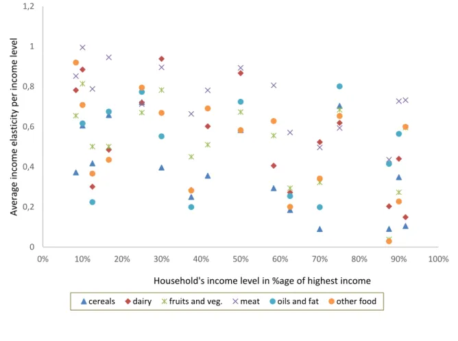
Then, price and income elasticities were estimated for different household income levels for 25 and 15 primary studies in our sample, respectively. This is illustrated on Figures 3 and 4, where income and own price elasticity estimates are reported with respect to household income levels. To make estimates from different studies comparable, income levels are represented as a percentage of the highest income considered in the study rather than as nominal income amounts. Indeed, high incomes in low GDP countries can be lower than low incomes in high GDP countries, and in most studies, incomes are not given in nominal values but in relative terms, i.e., income deciles or quartiles are considered, or a distinction is made between high, medium and low incomes. A slight decrease in income elasticities with household income appears in Figure 3, but no clear pattern arises for price elasticities in Figure 4. This suggests that price elasticities vary more (with GDP) across countries than (with household income) within countries.
Figure 3: Evolution of income elasticities with households’ income
0 0,2 0,4 0,6 0,8 1 1,2 0% 10% 20% 30% 40% 50% 60% 70% 80% 90% 100% Av era ge in come e las ticity p er in come le ve l
Household's income level in %age of highest income
20 Figure 4: Evolution of price elasticities with households’ income
3. Methodological sources of heterogeneity in elasticity estimates
Elasticity estimates collected from different primary studies display strong levels of heterogeneity, part of which can be attributed to the data based on which they have been estimated in terms of product and country or household income. However, as illustrated by the standard deviations reported in Tables 1 and 2 and by the dispersion of data in Figures 1 to 4, a significant proportion of the heterogeneity across elasticity estimates remains unexplained by these elements. We discuss here some characteristics that are essentially related to methodological issues that differ across the studies and that might be at the root of this additional heterogeneity across study estimates. These characteristics notably concern the flexibility of the functional forms used to represent household demand, the treatment of zero values in econometric estimations of demand systems, and the definition of the “price variable” used to estimate demand systems.
Diverse functional forms representing consumer demand are used in primary studies to estimate price and income elasticities. Among them is the Rotterdam model introduced by Barten (1964) and Theil (1965). The popularity of this model has already been noted by Clements and Gao
-1,4 -1,2 -1 -0,8 -0,6 -0,4 -0,2 0 0% 10% 20% 30% 40% 50% 60% 70% 80% 90% 100% Av era ge p rice elas ticity p er in come le ve l
Household's income level in %age of highest income
21
(2015), who review the methodological developments that have occurred over the past fifty years in applied demand analysis and demonstrate the importance of the Rotterdam model in this respect. This model is derived in an unconventional way in the sense that it does not require the specification of a specific type of cost or utility function. Other popular demand systems, such as the Linear Expenditure System (LES) (Stone, 1954), the Translog system (Christensen et al., 1975), and the Almost Ideal Demand System (AIDS) (Deaton and Muellbauer, 1980), are indeed more traditionally derived from the optimization of specific (indirect) utility or expenditure functions. Clements and Gao (2015), however, show that these systems can actually be reformulated as differential systems relatively similar to the Rotterdam model and can thus be considered to belong to the same class of differential demand systems as that of Rotterdam4.
Almost 7% of the primary studies included in our sample rely on the Rotterdam model. The LES and Translog systems are adopted in respectively 3% and 5% of the primary studies included in our sample. The AIDS and its linearized version, the LA-AIDS5, are the most well-represented demand systems, with 20% and 36% of primary studies relying on them, respectively. A generalization of the AIDS, the quadratic AIDS (QUAIDS) developed by Banks et al. (1997), is also used in 13% of the studies. In this model, budget shares are assumed to be quadratic functions of the log of income rather than linear functions, as they are in AIDS. This specification offers more flexibility in the representation of demand since income elasticities are allowed to vary with income levels. It should finally be noted that, contrary to ad hoc single equations sometimes used to estimate demand elasticities (in 5% of primary studies included in our sample), all the aforementioned demand systems are theoretically consistent since they have been built to satisfy the homogeneity, symmetry and adding-up constraints imposed by the economic theory of demand. The only theoretical property that might not necessarily be satisfied is the concavity in price of the expenditure function, which translates into the negative semi-definiteness of the Slutsky matrix. These restrictions can, however, be imposed in econometric estimations (see, e.g., Moschini (1998 and 1999) and Ryan and Wales (1998)).
4 The CBS model (Keller and van Driel, 1985) and the NBR model (Neves, 1994) are two other popular models
related to the Rotterdam model. Our sample, however, includes only one primary study relying on a CBS model and none that rely on an NBR model.
5 The LA-AIDS is an approximation of the AIDS in which the linear Stone price index is used in place of the
22
Finally, should be noted that 11% of the primary studies use other specific models to obtain demand elasticities6.
Furthermore, 18% of the studies rely on multi-stage budgeting frameworks that first allocate consumer food expenditures to broad product categories or groups based on group-specific price indices and then to smaller aggregates within each category, with within-groups budget allocation performed independently. By reducing the number of parameters to be estimated this nesting structure allows one to consider demand systems with more disaggregated products. It relies on the assumption of weak separability between goods, i.e., a change in price for one product in one category is assumed to affect the demand for all products in other categories in the same way, and on the assumption of low variability in group-specific price indices with expenditures (Edgerton, 1997). As emphasized by Edgerton (1997) and Carpentier and Guyomard (2001), multi-stage budgeting has important implications in terms of estimated income and price elasticities since specific formulas must be used to recover total or unconditional elasticities from estimates made for group or conditional elasticities. Given that our analysis focuses on the total impacts of income or price changes on food product demand, we consider only the unconditional elasticities estimates reported in primary studies. The specific structure of multi-stage budgeting frameworks and their underlying assumptions might however have some effects on these estimated unconditional elasticities.
Another methodological difference observed across the studies concerns the treatment of corner solutions. Datasets used to estimate demand models frequently contain a significant number of zeros since not all products are consumed by all consumers. This is all the more true when products are considered at disaggregated levels and in micro-econometric studies relying individual or household data. These zero values generate corner solutions, which can be a problem for econometric estimations of demand systems. This issue can be avoided by removing zeros in datasets by excluding the corresponding observations or by considering sufficiently aggregated data. This is the case for 35% of the studies included in our database. Other studies, however, tackle the issue and account for censored demand in their econometric
6 Among these models are the Florida model used by Seale et al. (2003a) and Muhammad et al. (2011), the LinQuad
model used by Fang and Beghin (2002) and Fabiosa and Jensen (2003), the CBS model used by Hahn (2001) and the AIDADS model used by Yu et al. (2004). Since these models are rarely used in our data, they have been grouped into a category termed “other” in our empirical application. Regarding the number of observations, this category is dominated by the Florida model since Seale et al. (2003a) and Muhammad et al. (2011) report 1,824 and 2,304 elasticity estimates, respectively.
23
estimations. Different means of addressing corner solutions have been proposed in the economic literature. In particular, Wales and Woodland (1983) and Lee and Pitt (1986), relying respectively on endogenous regime switching and virtual prices approaches, offer theoretically consistent frameworks to account for censored demands. However, these approaches are difficult to use in empirical applications, particularly when large datasets are considered. Empirical procedures have thus been developed to deal with censored demand, among which is the seminal work of Heien and Wessels (1990). A few years later, the approach proposed by Shonkwiler and Yen (1999) was published and is now commonly used in the literature. In the spirit of Heckman’s two-step estimator (1979), the estimator proposed by Shonkwiler and Yen (1999) involves first estimating a probit model and then conducting a regression that accounts for censoring through the introduction of correction terms that derive from the probit estimates. Although easy to implement, this estimator might lack efficiency, as do other two-step estimators (Wales and Woodland, 1983), and may lead to biased results in cases of distributional misspecification (Schafgans, 2004). Alternative approaches based, for instance, on simulated maximum likelihood approaches (Yen et al., 2003) and semiparametric econometrics (Sam and Zheng, 2010) have recently been proposed as means to overcome these issues.
The last methodological issue that deserves discussion relates to prices used to estimate demand systems. The datasets used to estimate demand systems do not generally explicitly contain price information mainly because prices paid by households are usually not directly observable and because goods are aggregated. A standard procedure involves using unit values (expenditures divided by quantities) as proxies for prices, but, as explained by Huang and Lin (2000), this is not fully satisfactory since other information related to food quality is given in unit values. One solution involves following the approach proposed by Deaton (1988), which allows one to extract quality effects from unit values. In spite of the potential biases induced by the use of unit values to estimate price elasticities, 95% of the studies still use them as proxies for product prices while 5% only rely on quality-adjusted prices as proposed by Deaton (1988).
To account for these methodological issues, we introduced into the database the following four additional variables: a “model” variable with eight modalities corresponding to the various functional forms used to model demand and three dummy variables indicating whether multi-stage budgeting, the treatment of corner solutions and quality adjusted prices, have been used in the primary studies.
24
We also added three dummy variables to account for the fact that econometric estimations of demand systems often include several variables in addition to prices and incomes. Control variables are indeed introduced in the primary studies’ econometric estimations for three main reasons. The dummy variables “hetero_indiv”, “hetero_time” and “hetero_product” indicate whether demographic characteristics have been used to control for heterogeneity across households, whether time dummies and trends have been used to account for the evolution of consumer demand and preferences over time and whether product brand or advertisement characteristics have been used to control for product heterogeneity, respectively.
Finally, Cornelsen et al. (2016) find estimation methods to have an impact on the estimated values of price elasticities. To control for this potential effect, we included in our database a variable reporting the econometric method used to conduct the estimations in the primary studies. We adopted the same classification as that used in Cornelsen (2016) to introduce a variable taking the following four modalities: seemingly unrelated regression (SUR), ordinary least squares regression, maximum likelihood estimation and other methods. We must, however, acknowledge that the distinction between the different methods is not always straightforward since, for instance, the iterative SUR estimation method often used to impose regularity condition on demand systems is asymptotically equivalent to a maximum likelihood approach. Here, we decided to classify iterative SUR methods under the “SUR” category.
4. Meta regression analysis
Having described the potential sources of heterogeneity across price and income elasticity estimates found in the literature, we perform an MRA of our data to identify and quantify these sources of heterogeneity in a statistically consistent manner.
4.1 Methodology
Two sets of MRA, one for price elasticities and one for income elasticities, are performed. The MAER-NET protocol (Stanley et al., 2013) identifies publication selection bias, heteroscedasticity and within-studies dependence as key issues to be approached through MRA. As explained in section 2.2, we use the PET test proposed by Egger et al. (1997) to test for publication selection bias. When publication bias is detected, it is accounted for by introducing
25
a measure of the precision of estimates as an explanatory variable in the MRAs in line with the method proposed by Stanley and Doucouliagos (2014).
Heteroscedasticity issues may arise during MRA because the variances of effect size estimates vary from one primary study to another for several reasons, including differences in sample size, sample observations or estimation procedures (Nelson and Kennedy, 2009). One straightforward means to account for this heteroscedasticity involves using a weighted least square (WLS) approach and to give more weight to the more precise estimate, i.e., to elasticity estimates with the lowest level of estimated variance. However, as noted above, very few studies included in our sample report variance in price and income elasticity estimates. We thus use primary studies’ sample sizes as proxies to these variances, which is a common procedure used in MRA studies and notably in environmental economics (Nelson and Kennedy, 2009). Other issues can arise in the presence of correlations of effect size estimates within and between primary studies. Indeed, our data contain several elasticity estimates collected from each primary study. However, if most characteristics distinguishing estimates from the same study (product category, household income level, demand functional form, econometric estimation method, etc.) are introduced as explanatory variables and thus are controlled for in our MRAs, some unobservable characteristics may give rise to correlated error terms across elasticities collected from the same primary study. In the same way, primary studies conducted by the same author may share unobservable characteristics and may lead to between studies correlations. To overcome this issue, we follow the same approach that was used by Disdier and Head (2008) and Cipollina and Salvatici (2010) and introduce random study/author effects into the MRA models. This results in the generation of mixed-effect models, which can be defined as multilevel regression models (Bateman and Jones, 2003) and are formally expressed as:
𝜃𝑖𝑗 = 𝛼0+ ∑ 𝛼𝑘𝑋𝑘 𝐾
𝑘=1
+ 𝑢𝑖+ 𝜀𝑖𝑗 (1)
where 𝜃𝑖𝑗 is the dependent variable and denotes the j-th (price or income) elasticity estimate collected from the i-th primary study (or i-th author), 𝛼0 is a fixed intercept and 𝛼𝑘 (𝑘 ∈ {1, … , 𝐾}) is the fixed effect coefficient associated with 𝐾 explanatory variable 𝑋𝑘 (𝑘 ∈
{1, … , 𝐾}). 𝜀𝑖𝑗 is normally distributed with constant variance and can be interpreted as a
sampling error term. 𝑢𝑖 is a random study (or author) effect that is normally distributed with constant variance independent of 𝜀𝑖𝑗 and is assumed to be uncorrelated with the explanatory variables. Adding this random effect to the MRA model allows one to account for correlations
26
between elasticity estimates of primary studies/authors (Nelson and Kennedy, 2009)7. In this
way, we also depart from the assumption that, conditional on the observed characteristics represented by the explanatory variables, all primary studies estimate exactly the same level of elasticity. Here, elasticity estimates are assumed to be comparable but not exactly the same across studies/authors (Nelson, 2013a), and the primary studies included in our data are assumed to form a random sample of a universe of potential studies (Borenstein et al., 2010). The soundness of this assumption was notably underscored by Higgins and Thompson (2002), who clearly argue for the introduction of random effects into MRA models. Nelson and Kennedy (2009) assert that mixed models may lead to bias fixed effect coefficient estimates if random effects are correlated with one or more explanatory variables. We assume that this is not the case here, which appears to be a reasonable assumption given that most of our explanatory variables are dummies representing characteristics that are not associated with only one author or study. Additionally, Nelson and Kennedy (2009, p. 358) conclude that “the advantages of random-effects estimation are so strong that this estimation procedure should be employed unless a very strong case can be made for its appropriateness”.
4.2 Test for publication bias
PET tests are performed to check for the presence of publication bias in our data. These tests involve regressing elasticity estimates on an inverse indicator of their precision. The following two sets of regressions are performed: one for price and one for income elasticities. Given the lack of standard errors of effect size estimates included in our data, we consider two alternative indicators of their precision including the inverse square root of the primary sample size and the inverse square root of DF. Stanley and Doucouliagos (2014) also recommend the use of WLS regressions with inverse standard errors as weights to deal with heteroscedasticity issues. We follow their proposed approach and use as weights the square roots of sample sizes or DF depending on which indicator we use for the regression.
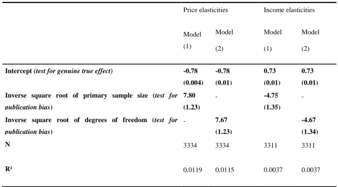
Estimation results are reported in Table 3. We find that the coefficients associated with the inverse precision criteria are significantly estimated in all cases, implying that publication selection bias exists in our data both for price (second and third columns of Table 3) and for income (fourth and fifth columns of Table 3) elasticities. Inverse precision indicators actually
7 The variance-covariance matrix of the composite error term of the model (𝑢
𝑖+ 𝜀𝑖𝑗) is block-diagonal allowing
27
appear to have a positive (resp. negative) impact on price (resp. income) elasticity estimates reported in the literature, i.e., to significantly lower the values of elasticities in absolute terms. It should also be noted that all constant terms are significantly estimated and have the expected signs, which are negative for price elasticities and positive for income elasticities, implying that food demand elasticities genuinely differ from zero beyond publication bias (Egger et al., 1997; Stanley, 2008). Finally, all these results are robust to the selection of primary sample sizes (second and fourth columns of Table 3) or DF (third and fifth columns of Table 3) as a precision indicator.
Publication bias is accounted for in subsequent MRAs by using an equivalent of the PEESE estimator proposed by Stanley and Doucouliagos (2014), in which inverse sample sizes are used as proxies to the variances of estimates.
Table 3: Test for publication bias - Estimation results
Price elasticities Income elasticities
Model (1) Model (2) Model (1) Model (2)
Intercept (test for genuine true effect) -0.78 (0.004) -0.78 (0.01) 0.73 (0.01) 0.73 (0.01) Inverse square root of primary sample size (test for
publication bias) 7.80 (1.23) - -4.75 (1.35) -
Inverse square root of degrees of freedom (test for
publication bias) - 7.67 (1.23) -4.67 (1.34) N 3334 3334 3311 3311 R² 0.0119 0.0115 0.0037 0.0037
Note: Model (1): Inverse square root of sample size used as proxy to standard error – Model (2): Inverse square root of DF used as proxy to standard error
4.3 Estimation results
The mixed-effect MRA models are estimated using the proc mixed Maximum Likelihood method implemented with SAS software.
Five quantitative variables and 14 nominal variables are used as explanatory variables in the MRAs. The five quantitative variables are the inverse squared root of primary sample sizes used
28
to correct for publication bias, the country’s GDP, the household income level and the two time trends corresponding to the publication date of the primary studies and to the decade of the data used to estimate elasticities. The 14 nominal explanatory variables are listed in Table 4. Most of these variables have already been discussed in section 3 except for the “Urban vs rural households” variable, which indicates whether the elasticity has been estimated for an urban population, a rural population or the general population without distinctions made between rural and urban areas. For each nominal variable, the modality serving as a baseline reference is highlighted in Table 4.
Table 4: Descriptive statistics of the variables introduced in the meta-regression- Summary statistics
Own price elasticities Income elasticities Average elasticity Nb Obs Average elasticity Nb Obs Type of data Panel -0.72 129 0.66 80 Cross section -0.58 2804 0.63 2900 Time series -0.66 401 0.69 331 Data level Individual -0.70 1154 0.70 1153 Country -0.47 2180 0.59 2158 Product Dairy -0.59 419 0.72 412
Fruits and vegetables -0.61 668 0.61 694
Meat and fish -0.57 945 0.73 946
Oils and fats -0.44 338 0.46 326
Other food products -0.67 444 0.77 424
Cereals -0.52 520 0.45 509
Product aggregation level
Product level -0.68 1263 0.69 1253
29
Own price elasticities Income elasticities Average elasticity Nb Obs Average elasticity Nb Obs Region Latin America -0.50 247 0.65 371 East Asia -0.66 425 0.73 506 Asia Other -0.60 609 0.59 542 European Union -0.43 541 0.52 521 Europe Other -0.57 78 0.34 78
Former Soviet Union -0.49 224 0.64 224
Middle East -0.64 257 0.57 188
North Africa -0.49 35 0.63 35
Sub-Saharan Africa -0.61 464 0.75 500
Oceania -0.33 42 0.43 42
North America -0.61 412 0.65 304
Urban vs rural households
Urban -0.62 360 0.64 346 Rural -0.62 321 0.76 385 No distinction -0.55 2653 0.61 2580 Demand model LA-AIDS -0.71 503 0.82 388 AIDS -0.84 575 0.79 229 QUAIDS -0.78 449 0.64 319 Rotterdam -0.44 33 0.34 36 Translog -0.71 65 0.97 61 Single equation -0.90 49 0.51 68 Other -0.46 1883 0.58 1990 CES or LES -0.31 243 0.55 220
Zero demands accounted for
Yes -0.77 335 0.68 283
30
Own price elasticities Income elasticities Average
elasticity Nb Obs
Average
elasticity Nb Obs
Prices adjusted for quality
Yes -0.62 165 0.80 200
No -0.57 3191 0.62 3111
Individuals’ characteristics included
Yes -0.57 2933 0.62 2735
No -0.64 401 0.71 576
Products’ characteristics included
Yes -0.58 24 0.99 16
No -0.57 3310 0.64 3295
Time variables included
Yes -0.84 308 0.71 344 No -0.55 3026 0.63 2967 Multi-stage budgeting Yes -0.55 2356 0.58 2082 No -0.64 978 0.72 1229 Econometric method
Least Square regression -0.41 295 0.62 337
SUR -0.73 685 0.74 577
Other method -0.74 248 0.70 315
Maximum Likelihood -0.50 2106 0.60 2082
Estimation results are presented in Table 5 for price elasticities and in Table 6 for income elasticities. In both tables, the second column (Model (1)) reports the estimated coefficient of our “baseline” mixed effect MRA model. In this model, random primary study effects are included, publication bias is accounted for by using the inverse primary sample sizes as
31
explanatory variables, and sample sizes are also used as weights to correct for heteroscedasticity issues. The other columns of Tables 5 and 6 report the results of estimations that have been conducted to test the sensitivity of our results to the specifications of Model (1). More precisely, the third column (Model (2)) reports estimation results obtained without accounting for publication bias. The fourth column (Model (3)) reports estimation results obtained by using DF instead of sample sizes to weight observations. In Model (4), random author effects are included instead of random study effects, and in Model (5), both random study and author effects are included, with the study effect being nested within the author effect. Model (6) is a fixed effect-size MRA, i.e., no random effects are introduced to account for correlations between elasticity estimates within primary studies or authors. Models (7) and (8) are estimated to test the sensitivity of our results to the treatment of outliers. Indeed, as did Cornelsen et al. (2015), we considered price and income elasticities that ranged outside three standard deviations of their respective averages as outliers and excluded them from our sample. Model (7) is estimated for a sample for which outliers are treated by using another approach, which is a trimming method similar to that used by Nelson (2013). The trimming method involves excluding 10% of observations from the sample, i.e., the largest elasticities (2.5% of the observations), the smallest elasticities (2.5%), the elasticities with largest standard errors (or the smallest sample sizes in our case) (2.5%) and the elasticities with lowest standard errors (or the largest sample sizes in our case) (2.5%). This method leads to the exclusion of 307 price elasticities and 287 income elasticity estimates compared to 63 and 41 estimates respectively, that were excluded with the “three standard deviations rule”. Finally, Model (8) is estimated for a sample for which no outliers are excluded.
Table 5: MRA of price elasticities – estimation results
Model (1) Model (2) Model (3) Model (4) Model (5) Model (6) Model (7) Model (8) Quantitative variables Intercept -0.25 (0.15) -0.36 (0.15) -0.25 (0.15) -0.16 (0.17) -0.25 (0.15) -0.33 (0.06) -0.02 (0.15) -0.32 (0.18)
Publication bias correction term -14.95 (5.73) -15.20 (5.76) -14.87 (5.82) -14.96 (5.73) -1.21 (2.52) -49.93 (11.23) -8.57 (6.86)
Publication date trend (1976=1) -0.004 (0.005) -0.004 (0.005) -0.004 (0.01) -0.002 (0.003) -0.004 (0.005) -0.003 (0.001) -0.010 (0.005) -0.010 (0.01)
Data decade trend (1950’s=1) 0.03 (0.03) 0.03 (0.03) 0.03 (0.03) 0.03 (0.02) 0.03 (0.03) 0.04 (0.01) 0.002 (0.03) 0.04 (0.03)