High performances combinatorics using GPUs

HAL Id: hal-01917588

https://hal.archives-ouvertes.fr/hal-01917588

Submitted on 9 Nov 2018

HAL is a multi-disciplinary open access

archive for the deposit and dissemination of

sci-entific research documents, whether they are

pub-lished or not. The documents may come from

teaching and research institutions in France or

abroad, or from public or private research centers.

L’archive ouverte pluridisciplinaire HAL, est

destinée au dépôt et à la diffusion de documents

scientifiques de niveau recherche, publiés ou non,

émanant des établissements d’enseignement et de

recherche français ou étrangers, des laboratoires

publics ou privés.

Daniel Vanzo

To cite this version:

Daniel Vanzo. High performances combinatorics using GPUs. [Technical Report] LRI, Univ.

Paris-Sud, CNRS, Inria, Université Paris-Saclay. 2018. �hal-01917588�

High performances combinatorics using GPUs

HPCombi On GPU

Author :

Contents

1 Introduction 1

2 Transformation semigroups exploration 1

3 GPU Algorithms 2 3.1 General algorithm . . . 2 3.2 Composition . . . 3 3.3 Hashing . . . 5 3.4 Transformations equality . . . 5 3.5 Duplicates’ elimination . . . 6 4 Profiling results 8 5 Conclusions 10 6 Sources 10

Appendix A: Basics of GPU architecture 11

1. INTRODUCTION Daniel Vanzo

1

Introduction

Semigroups and monoids are algebraic structures consisting of a set and an associative binary operation. Monoids have the additional property that they contain a neutral element for the latter binary operation. Semigroups and monoids are studied notably in the theory of finite automata and formal language [10]. Several libraries, like libsemigroups [8] or HPcombi[6], are available to manipulate such objects, they allow good performances using advanced algorithms and CPU (Central Processing Unit) vector instructions.

This document describes an attempt to port some related routines to GPU (Graphics Processing Unit), in particular the ones involved in the exploration of transformation semigroups [10]. Section 2 sets the problem of transformation semigroups exploration, section 3 gives a detailed description of the algorithms used on the GPU. In section 4 profiling results are compared and shows that GPU allow significant speedup for some routines, finally, in section 5 we conclude and note that the benefit offered by GPU is highly dependent on ”how much” of the global algorithm is ported to GPU.

2

Transformation semigroups exploration

Transformations on [1,n] are stored as an array, for instance with n=4:

The array 2|4|1|3 represents the transformation that sends 1 on 2, 2 on 4, 3 on 1 and 4 on 3. Let G = {g1, g2, . . . , gng} be a set of transformations called generators, where ng is the number

of generators. We aim at finding properties about the set of transformations generated by the compositions of those generators. The composition of two transformation g2◦ g1 can be seen as

the shuffling of g2 according to g1 :

g1 = 2|4|1|3

g2 = 1|3|4|2

g2◦ g1 = 3|2|1|4

The algorithm starts by defining an initial set of transformations F0 only containing the

identity transformation Id = 1|2|3| . . . |n. Let’s name k the stage number. At each stage of the algorithm all new transformations from this set Fk are composed with all generators from G. The

transformations are considered as new if there are in Tk= Fk\Fk−1. Initially T0= F0= {Id}

At stage number k, all element of Tk are composed with all generators in G. The resulting

transformations are then compared with transformations in Fk and added, if absent, in Fkto form

Fk+1.

To each transformation in Fkwe associate a suite of generators of lengh k, that permitted

its computation. A word is defined as a suite of generators to be composed with the identity transformation, Id. For instance the word [5, 3, 8, 4] applied to Id would be the transformation g5◦ g3◦ g8◦ g4◦ Id, computing this transformation will also be described as computing the word.

A particular transformation can be obtained from several different words. The first words from which a particular transformation is obtained, is stored in a hash table. The key for the hash table is set to be a structure containing a hash value and a word. This particular structure has been chosen rather than a dictionary data-structure for the following reasons:

• The hash value allows fast distinction of keys when hash value are different whitout computing the transformations.

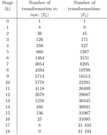
Stage (k) Number of transformation to test: |Tk| Number of transformations: |Fk| 0 1 1 1 8 9 2 36 45 3 126 171 4 356 527 5 860 1387 6 1464 3151 7 3054 6205 8 4594 10799 9 5714 16513 10 5778 22291 11 4118 26409 12 2678 29087 13 1258 30445 14 486 30931 15 136 31067 16 25 31095 17 8 31 103 18 0 31 103

Table 1: Transformation semigroup exploration progression.

• Storing the word in the key structure allows to compute transformations and reliably compare them.

Detailed discussion about keys comparison is in subsection 3.4.

All transformations composition occurring at stage k can be computed in parallel, there are (|G| × |Tk|) of them. After composing the transformations, all hash value can be computed

in parallel as well. Depending on the hash table implementation, keys can, or not, be inserted in parallel in the hash table.

The first implementation of the algorithm uses Google Sparsehash [5] as the hash table, which only allows for sequential insertions. Further implementation could use a hash table on the GPU as shown in [11] which allow for parallel insertion.

Table 1 illustrates a transformation semigroup exploration for the test case Bihecke 5 (details about test cases are in section 4). There are 8 generators of lengh 120. At stage 1, T1= G

and F1 = G ∪ {Id}. Among the |T1| × |G| = 8 ∗ 8 words tested in stage 2, 36 new words have

been found and added in F2, which means 64 − 36 = 28 transformations where duplicates. The

algorithm runs until there is no new transformation to test (|Tend| = 0), meaning the previous

stage did not permit to found any new transformation (|Fend−1| = |Fend|).

3

GPU Algorithms

3.1

General algorithm

The general transformation semigroups exploration algorithm is described in Algorithm 1. Recall that G is the set of generators.

3. GPU ALGORITHMS Daniel Vanzo

Algorithm 1 Transformation semigroups exploration

F0= {Id}

T0= {Id}

for 0 < k < maxStage do

- Compose all transformations in Tk with all transformations in G, resulting in a set of

trans-formations called TMP.

- Compute the hash values of all transformations in TMP.

- Search for duplicates within TMP and eliminate them from TMP. This step is not done in all implementations, see section 4 for more details.

- Try inserting transformations from TMP into Fk+1and compute Tk+1= Fk+1\Fk

if |Tk+1| = 0 then

Stop

end if end for

3.2

Composition

Let’s assume one thread should compute a word. Two loops are necessary: one to iterate over the generators in the word, the second to iterate over the transformations coefficients. The loops are intergengeable, let’s compare both possibilities. Algorithm 2 shows the algorithm for which the outer loop iterates over the generators and the inner loop iterates over the coefficients:

• A temporary array resultTMP must be allocated to store intermediate results. • Multiple loops over the coefficients are needed to :

1. Initialize the result array to identity, 2. Compose with one generator,

3. Copy temporary results into the result array.

• Access to the generators array is only done once per generator, • Accesses to the generators component are contiguous,

• Parallelization of the outer loop require synchronization of all treads at each iteration.

Algorithm 3 shows the algorithm for which the outer loop iterates over the coefficients and the inner loop iterates over the generators:

• No temporary array is needed, memory consumption is halved compared to Algorithm 2, • Only one loop over the coefficients is needed,

• Multiple access to the same generator are done, as many as the lenght of the transformations, • Accesses to the generators component are not contiguous,

• The outer loop can easily be parallelized without need for explicit synchronization.

GPU threads can be synchronized in a CUDA block whereas threads in different CUDA blocks can’t be synchronized [1] (details about GPU architecture are in section A). Indeed, there is no guarantee CUDA blocks are executed in parallel, as a consequence, synchronization between CUDA blocks could lead to dead blocks. Hence, a parallel implementation of Algorithm 2 would require transformations coefficients to be spread over a maximum of 1024 threads, the maximum

number of threads in a CUDA block. Whereas, a parallel implementation of Algorithm 3 could spread transformations coefficients over 1024 × 231 _{threads, the maximum number of thread in a}

CUDA block times the maximum number of CUDA block following the first dimension.

The later limitation on parallelism, the doubling of memory consumption and the need for three loops over the coefficients in Algorithm 2 made us choose the Algorithm 3 for the starting point of the parallel implementation. This leading to Algorithm 4, a parallelized version for GPU of Algorithm 3. The outer loop is basically replaced by a ”if” statement selecting threads that should compute the instructions. Each thread applies all compositions to one coefficient. To adapt granularity, Algorithm 3 and Algorithm 4 can be mixed to assign several coefficients to each thread on which to compose all generators in a word.

As the results of several words are requested at one stage, more parallelism can be ex-ploited. Indeed, each word can be computed in parallel. Hence, two levels of parallelism can be exploited: parallelism over several words and parallelism over coefficients of the transformations. A good balance between both should be found:

• When few words are to be computed, transformations coefficients should be spread over lots of threads to exploit parallelism,

• When lots of words are to be computed, transformations coefficients should be assigned to few threads for greater granularity.

In our implementation of the exploration of the transformation semigroups, parallelism is dynamically tuned during the execution according to the number of word to be computed.

Algorithm 2 Composition: Outer loop on generators, inner loop on coefficients

// Initialise Id //

for 0 < coef < size do

result(coef ) = coef

end for

for 0 < j < sizeW ord do

gen = word(j)

// Compute the word and same result to temporary array //

for 0 < coef < size do

index = gen(coef )

resultT M P (coef ) = result(index)

end for

// Copy temporary array to result array //

for 0 < coef < size do

result(coef ) = resultT M P (coef )

end for end for

Algorithm 3 Composition: Outer loop on coefficients, inner loop on generators for 0 < coef < size do

index = coef

for 0 < j < sizeW ord do

gen = word(j) index = gen(index)

end for end for

3. GPU ALGORITHMS Daniel Vanzo

Algorithm 4 Composition: Outer loop on coefficients, inner loop on generators with multiple

threads

if 0 < threadId < size then

index = threadId

for 0 < j < sizeW ord do

gen = word(j) index = gen(index)

end for end if

3.3

Hashing

Let t be a transformation and Ptbe the polynomial n

X

i=1

t(i)Xi, where n is the lengh of the

trans-formation. The hash function is defined as hash(t) = Pt(prime), where prime is a prime number.

The polynomial value is computed with the Ruffini-Horner method [2]. Parallelism is obtained

Algorithm 5 Hashing

prime = P rimeN umber result = prime × trans(0)

for 1 < i < size do

result += trans(i) result ∗= prime

end for

by assigning one hash value computation per thread. More parallelism coull be exploited by dy-namically tuning parallelism during the execution as done for the words’ computation. This is not trivial because the computation of a hash value involves overflows. As a consequence, a direct parallelization of Algorithm 5 would give different results depending on the number of threads used for a hash value computation. Dynamically adapting the number of thread computing a hash value would lead two false results. A more advanced algorithm is needed, assuring the exact same overflows occur regardless of the number of threads involved in the hash value computation. As the hash values computation is not a bottleneck in our examples, this has not been tested, each threads computes a hash value regardless of the size of the transformations.

3.4

Transformations equality

When inserting a new key in the hash table, tests for keys equality are performed. Remind that a key is a structure containing a hash value and a word. To compare two keys, the hash values are first compared. If they are different, transformations are different. If the hash values are identical the transformations have to be compared coefficient by coefficient to reliably discriminate them. The word contained in the key structure allows to compute both transformations and compare them coefficient by coefficient as shown in Algorithm 6. This latter is a sequential version of the algorithm. In the GPU version each thread computes one coefficient for both transformations according to Algorithm 4. Then each thread compares the resulting coefficients and store the result in the equal variable. The sum of each thread’s equal variable is then computed and compared to the size of the transformations.

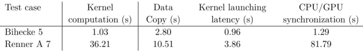
The execution time of the equality test on GPU is dominated by CPU/GPU data copy, kernel launching latency and CPU/GPU synchronization. This is demonstrated in Table 2, which is a profiling of the execution of the Bihecke 5 and Renner A 7 test cases (details about test cases

Test case Kernel computation (s) Data Copy (s) Kernel launching latency (s) CPU/GPU synchronization (s) Bihecke 5 1.03 2.80 0.96 1.29 Renner A 7 36.21 10.51 3.86 81.79

Table 2: Profiling of the equality testing kernel on GPU for the Bihecke 5 and Renner A 7 test cases.

Test case Size Time on CPU (s) Time on GPU (s)

Bihecke 5 120 0.187 < 3.37

Bihecke 6 (partial) 720 38.3 < 219

Renner A 6 13 327 7.85 > 1.11

Renner A 7 130 922 1320 > 45.6

Table 3: Time comparison of the equality testing kernel on GPU and CPU for the Bihecke 5, Bihecke 6, Renner A 6 and Renner A 7 test cases.

are in section 4). Testing equality on CPU avoids the overhead of copying data to the GPU, kernel launching latency and CPU/GPU synchronization. Table 3 compares the time to test for equality in different test cases, when run on the CPU on one hand and on the GPU, on the other hand. When transformation sizes are small (120, 720) equality testing is faster on CPU, when transformation sizes are big (13 327, 130 922) it is faster on GPU.

All runs in this section are executed on a Intel Xeon E5-1650 (2012) as the CPU and on a NVIDIA GTX 1080 (2016) as the GPU (details about the configuration are in appendix B).

Algorithm 6 Equality testing if 0 < threadId < size then

index1 = threadId index2 = threadId equal = 0

for 0 < j < sizeW ord do

gen1 = word1(j) gen2 = word2(j) index1 = gen1(index1) index2 = gen2(index2)

end for

if index1 = index2 then

equal = 1

end if end if

Sum(equal)

3.5

Duplicates’ elimination

At each stage, new computed transformations are inserted in the hash table located on the CPU. This requires testing if the hash table location attributed to the transformation is empty, intro-ducing a memory fetch. Those memory fetches are random as a consequence of the hash function efficiency. When the hash table is big enough, it doesn’t fit entirely in the CPU cache and lots of cache misses occur. To limit the number of cache misses, the number of insertion attempts in the hash table should be lower. For that purpose, a kernel is executed on the GPU to eliminate dupli-cates within the set of transformations computed at a particular stage. This kernel is described in

3. GPU ALGORITHMS Daniel Vanzo

Test case Size Total pourcentage of

eliminated transformations Bihecke 5 120 64% Bihecke 6 (partial) 720 69% Renner A 6 13 327 64% Renner A 7 130 922 66%

Table 4: Efficiency of the duplicates’ elimination kernel for the Bihecke 5, Bihecke 6, Renner A 6 and Renner A 7 test cases.

Algorithm 7. As a result, the set of transformations the CPU attempts to insert in the hash table is smaller. Table 4 shows that the number of transformations the CPU attemps to insert is about 3 times smaller in typical test cases (details about test cases are in section 4).

In our implementation, hash value are computed before the elimination of duplicates. This allows the duplicates’ elimination algorithm to first compare hash value before comparing the transformations coefficients by coefficients. The downside of this functions ordering is that some hash value computation could be avoided. Indeed, if the duplicates’ elimination algorithm is run before computing the hash value, 3 times less hash value would be computed. Benchmarks in section 4 show that the hash values computation is cheap compared to the elimination of duplicates, hence computing the hash value first to accelerate duplicates’ elimination is the better choice.

As for the composition algorithm, a GPU version of Algorithm 7 is obtained by replacing the outer loop with a ”if” statement selecting threads that should compute the instructions.

Note that the inner loop iterating over the coefficients of a transformation in Algorithm 7, could be stopped the first time a non equality occurs. This happened to be much slower for the test cases described in section 4. Two hypothesis, yet to be confirmed, could explain why :

• The additional loop control instructions resulting from the break instruction are not efficiently handled by the GPU.

• The break instruction results in more warp divergence, which implies serialization of execution [1] (details about GPU architecture are in appendix A).

Algorithm 7 Eliminating duplicates for 0 < trans < nb trans do

equal = 0

for 0 < other < trans do

if hash(trans) = hash(other) then for 0 < i < size do

if trans(i) = other(i) then

equal += 1

end if end for

if equal = size then

Suppress trans

end if end if end for end for

4

Profiling results

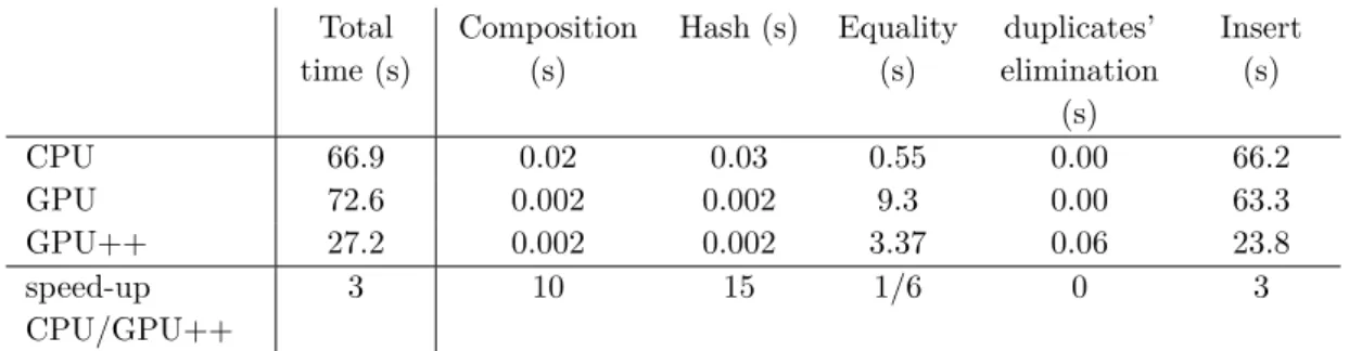
In this section the whole algorithm of transformation semigroup exploration is profiled. The algorithm parts described in subsection 3.2, subsection 3.3, subsection 3.4 and subsection 3.5 are profiled as well as the insertion time in the hash table. Three implementations are compared:

1. The whole algorithm is executed on the CPU (composition, hashing, equality testing routines and hash table) with non optimized code. No duplicate elimination is executed. This is the reference implementation named ”CPU”.

2. The composition, hashing and equality testing routinesare axecuted on GPU and the hash table is located on the CPU. No duplicate elimination is executed. This implementation is named ”GPU”.

3. The composition, hashing and equality testing routines are executed on GPU and the hash table is located on the CPU. Duplicate elimination is executed on the GPU. This implemen-tation is named ”GPU++”.

The four test cases are the following:

• Bihecke 5: 8 generators of lengh 120, generating a set of 31 103 transformations, • Bihecke 6: 10 generators of lengh 720, generating a set of 7 505 009 transformations, • Renner A6: 6 generators of lengh 13 327, generating a set of 13 327 transformations, • Renner A7: 7 generators of lengh 130 922, generating a set of 130 922 transformations.

All runs in this section are executed on a Xeon E5-1650 as the CPU and on a GTX 1080 as the GPU. The test case Bihecke 6 requires running several weeks to complete, whereas for this study runs where done only for a few hours. As a consequence results about Bihecke 6 are partial: they are the results obtained at stage 12.

Tables 5 to 8 show that a noticeable speed-up is obtained from the GPU for the Compo-sition and Hashing routines. Conclusions need to be mitigated, first because the CPU routines are not optimized, second because the overall time proportion of those two routines is low.

As discussed in subsection 3.4, the equality testings are longer on the GPU when transformations are rather small (Tables 5 and 6), faster on the GPU when transformations are rather big (Tables 7 and 8).

For the Bihecke 5 and Bihecke 6 (Tables 5 and 6) test cases, the overhead of the duplicates’ elimination routine is negligible compared to the total execution time (< 1%). For the Renner A 6 and Renner A 7 (Tables 7 and 8) test cases, the overhead of the duplicates’ elimination routine is low (< 10%) but not negligible. In all test cases, the duplicates’ elimination routine allow a speed-up over 3 for the hash table insertion time. This is because about 2/3 of the transformations computed at each stage are eliminated as duplicates on the GPU. Details are in subsection 3.5. Table 8 shows a speed-up of 5 when using the duplicates’ elimination routine because of an unexpectedly high insertion time for the CPU implementation. This remains unexplained as for now.

4. PROFILING RESULTS Daniel Vanzo Total time (s) Composition (s) Hash (s) Equality (s) duplicates’ elimination (s) Insert (s) CPU 66.9 0.02 0.03 0.55 0.00 66.2 GPU 72.6 0.002 0.002 9.3 0.00 63.3 GPU++ 27.2 0.002 0.002 3.37 0.06 23.8 speed-up CPU/GPU++ 3 10 15 1/6 0 3

Table 5: Profiling of the test case Bihecke 5 for three implementations.

Total time (104_s) Composition (s) Hash (s) Equality (s) duplicates’ elimination (s) Insert (104 _s) CPU 12.3 5.75 15.6 151 0.00 12.3 GPU 12.3 0.258 0.858 712 0.00 12.3 GPU++ 4.08 0.259 0.842 220 155 4.04 speed-up CPU/GPU++ 3 22 15 2/3 0 3

Table 6: Profiling of the test case Bihecke 6 (partial) for three implementations.

Total time (s) Composition (s) Hash (s) Equality (s) duplicates’ elimination (s) Insert (s) CPU 46.3 1.22 2.12 32.6 0.00 9.88 GPU 12.6 0.068 0.066 3.24 0.00 9.16 GPU++ 4.64 0.062 0.065 1.09 0.381 3.03 speed-up CPU/GPU++ 10 20 33 30 0 3

Table 7: Profiling of the test case Renner A6 for three implementations.

Total time (s) Composition (s) Hash (s) Equality (s) duplicates’ elimination (s) Insert (s) CPU 8 440 260 238 5 870 0.00 1 990 GPU 1 390 10.2 12.7 155 0.00 1 170 GPU++ 524 10.2 12.7 45.9 22.1 391 speed-up CPU/GPU++ 16 25 19 128 0 5

5

Conclusions

For all test cases, the composition and hashing routines benefit from the use of GPU. The speedups (from 10 to 33) should be interpreted with care as the reference CPU routines are not optimized. The equality testing routine benefits greatly (speedups up to 128) from GPU when the transfor-mations are very big (13 327, 130 922). Conversely, when the transfortransfor-mations are quite small (120, 720) the equality testing on GPU is slower than on CPU.

As the insertion time is dominant in the total execution time (due to cache misses, see subsection 3.5), the duplicates’ elimination on GPU is quit valuable. For the Bihecke (5 and 6) test cases, the total speed-up is actually equal or very close to the insertion time speed-up: 3. For the Renner (6 and 7) test cases, duplicates’ elimination allows to noticeably reduce the equality checking time. Note that similar speed-ups could not have been obtained on the CPU with this hash table implementation (Google Sparsehash [5]). Indeed, this hash table implementation only allows sequential insertion, furthermore, memory latency is a bottleneck even for sequential insertion. It is the fast GPU memory random accesses that permit those speed-ups.

For some routines, the benefit from GPU is degraded by the CPU/GPU copy and syn-chronization time. Hence, the more routines ported on GPU the better the performance are, as fewer communications and syncrhonisations would be required. In our particular application, ran-dom accesses to CPU RAM memory is the bottleneck. Further work could focus on addressing this bottleneck from two angles:

• Locating the hash table on the GPU [11], • Using another data structure like Tries [3].

6

Sources

The source code is hosted on the rennergpu branch of HPCombi Github repository. It can be cloned with this command:

6. SOURCES Daniel Vanzo

Appendix A: Basics of GPU architecture

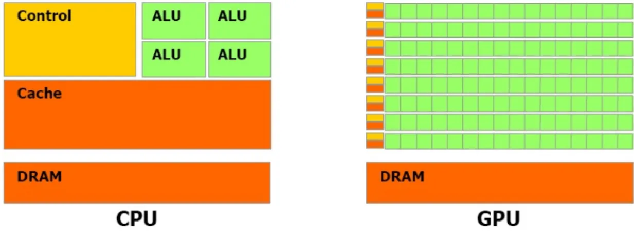
Figure 1 and Table 9 show the main differences between CPUs and GPUs. A GPU can contain up to several thousand Arithmetic logic units (ALU), whereas CPU contain a few dozens. The GPU global memory (comparable to RAM memory on CPUs) is on the same chip as the ALUs, thus allowing high bandwidth. CPUs often operate at faster clock speeds than GPUs.

CPU :

• CPU cores : 2 to 72,

• RAM bandwidth : 8 to 540 Go/s, • Clock frequency : 1 200 to 3 500 MHz.

GPU :

• CUDA cores : 250 to 5 120,

• Global memory bandwidth : 160 to 900 Go/s,

• Clock frequency : 745 to 1 480 MHz.

Table 9: Comparison of typical specifications of CPUs and GPUs

Figure 1: Schematic of CPU and GPU architectures . (source : [1])

NVIDIA GPU are organized as follows [1] :

1. A GPU is composed of several Streaming Multiprocessor (SMX) (15 on NVIDIA Tesla K40 (2013)).

2. A SMX executes several threads blocs. The number of threads blocks executed on a SMX is not directly available to the programmer. Shared memory and register usage by the kernel are the two factor limiting the number of blocks executed on a SMX. On the Kepler architecture 65 536 registers and 48 Kbytes of shared memory are available on a SMX.

3. The L2 cache is common to all SMX and the L1 cache is common to all threads within a SMX.

4. A CUDA block contains several threads (up to 1 024). The block size is set by the programmer in 3 dimensions. It is a parameter to optimize. Shared memory is a memory bank shared over all threads from a block.

5. Blocks are organized in a 3 dimensions grid also set by the programmer. Figure 2 illustrates the threads organization in a grid of blocks.

6. A warp is a group of 32 threads of a block. All thread in a warp execute the same instructions according to the SIMT (Single Instruction Multiple Threads) [4] protocol.

6. SOURCES Daniel Vanzo

Appendix B: Specifications of the GPUs and CPUs used in

this study

GPU K40 [9] 2×CPU Xeon E5-2620 v2 [7]

Launch year 2013 2012

Architecture Kepler Ivy Bridge

SMX/CPU Cores 15 2×6

CPU threads X 2×12

CUDA Cores 2880 X

Frequency (GHz) 0.74 2.1

Global memory/RAM size (Go) 12 64

Global memory/RAM max bandwidth (Go/s) 288 51

References

[1] CUDA C programming guide. NVIDIA, 2017.

[2] Peter Borwein and Tam´as Erd´elyi. Polynomials and polynomial inequalities, volume 161. Springer Science & Business Media, 2012.

[3] Rene de la Briandais. File searching using variable length keys.

[4] L. Erik, N. John, O. Stuart, and M. John. Nvidia tesla: A unified graphics and computing architecture. IEEE micro, 28(2), 2008.

[5] Google. Sparsehash. https://github.com/sparsehash/sparsehash. Accessed: 2018-08-03. [6] Florent Hivert. HPCombi. https://github.com/hivert/HPCombi. Accessed: 2018-08-03. [7] INTEL. Intel XeonR Processor E5-2600 v2 Product Family, 2012.R

[8] J. D. Mitchell and M. Torpey. libsemigroups. https://github.com/james-d-mitchell/ libsemigroups. Accessed: 2018-08-03.

[9] NVIDIA. Tesla K40 GPU active accelerator, 2013.

[10] Jean- ´Eric Pin. Mathematical foundations of automata theory. Lecture notes LIAFA, Univer-sit´e Paris, 7, 2010.