HAL Id: hal-03210283
https://hal.archives-ouvertes.fr/hal-03210283
Submitted on 4 Jun 2021
HAL is a multi-disciplinary open access archive for the deposit and dissemination of sci-entific research documents, whether they are pub-lished or not. The documents may come from teaching and research institutions in France or abroad, or from public or private research centers.
L’archive ouverte pluridisciplinaire HAL, est destinée au dépôt et à la diffusion de documents scientifiques de niveau recherche, publiés ou non, émanant des établissements d’enseignement et de recherche français ou étrangers, des laboratoires publics ou privés.
Implications for Deriving Regional Fossil Fuel CO 2
Estimates from Atmospheric Observations in a Hot Spot
of Nuclear Power Plant 14 CO 2 Emissions
Felix Vogel, Ingeborg Levin, Doug Worthy
To cite this version:
Felix Vogel, Ingeborg Levin, Doug Worthy. Implications for Deriving Regional Fossil Fuel CO 2 Estimates from Atmospheric Observations in a Hot Spot of Nuclear Power Plant 14 CO 2 Emissions. Radiocarbon, University of Arizona, 2016, 55 (3), pp.1556-1572. �10.1017/S0033822200048487�. �hal-03210283�
IMPLICATIONS FOR DERIVING REGIONAL FOSSIL FUEL CO2 ESTIMATES FROM
ATMOSPHERIC OBSERVATIONS IN A HOT SPOT OF NUCLEAR POWER PLANT
14CO2 EMISSIONS
Felix R Vogel1,2 • Ingeborg Levin3 • Doug E J Worthy1
ABSTRACT. Using 14
C observations to infer the local concentration excess of CO2 due to the burning of fossil fuels
( FFCO2) is a promising technique to monitor anthropogenic CO2 emissions. A recent study showed that 14
CO2 emissions
from the nuclear industry can significantly alter the local atmospheric 14
CO2 concentration and thus mask the 14
C depletion due to FFCO2. In this study, we investigate the relevance of this effect for the vicinity of Toronto, Canada, a hot spot of
anthropogenic 14CO
2 emissions. Comparing the measured emissions from local power plants to a global emission inventory
highlighted significant deviations on interannual timescales. Although the previously assumed emission factor of 1.6 TBq(GWa)–1 agrees with the observed long-term average for all CANDU reactors of 1.50 ± 0.18 TBq(GWa)–1. This power-based parameterization neglects the different emission ratios for individual reactors, which range from 3.4 ± 0.82 to 0.65 ± 0.09 TBq(GWa)–1. This causes a mean difference of –14% in 14CO
2 concentrations in our simulations at our observational
site in Egbert, Canada. On an annual time basis, this additional 14
CO2 masks the equivalent of 27–82% of the total annual
FFCO2 offset. A pseudo-data experiment suggests that the interannual variability in the masked fraction may cause spurious
trends in the FFCO2 estimates of the order of 30% from 2006–2010. In addition, a comparison of the modeled 14C levels
with our observational time series from 2008–2010 underlines that incorporating the best available 14CO
2 emissions
significantly increases the agreement. There were also short periods with significant observed 14C offsets, which were found
to be linked with maintenance periods conducted on these nuclear reactors. 1. INTRODUCTION
Over the past 2 decades, the global total emissions of CO2 from fossil fuel burning have increased from 6.45 PgC in 1990 to 8.75 PgC in 2008 as reported by the Carbon Dioxide Information Analysis Center (CDIAC; http://cdiac.ornl.gov/trends/emis/annex.html). This global emission incre ase of 36% is rather sobering given the considerable efforts made by signatory nations within the Kyoto protocol to rather reduce fossil fuel CO2 emissions. In fact, the statistical data indicate that there are stark differences of the emission trends in different countries and regions. While Annex B countries (i.e. most of Europe, North America, and other industrialized countries) have reported almost constant emissions of 3.90 to 3.88 PgC/yr, emissions from the Non-Annex B countries (i.e. China, India, and developing countries) have more than doubled from 2.11 PgC in 1990 to 4.60 PgC in 2008, as reported by CDIAC. It is apparent that investigation of emissions and their trends requires regional-scale evaluation. The scientific community has begun moving towards independent validation of the published emission statistics using atmospheric observations (Levin and Rödenbeck 2008; Weiss and Nisbet 2010). This effort will be even more important as the statistical data from the Non-Annex B countries is subject to larger uncertainties than that in industrialized countries (Marland et al. 2009; Guan et al. 2012). To quantify the emissions of fossil fuel CO2 on a local and regional scale, measuring the depletion of the 14C/C ratio in ambient CO
2 due to the local surplus of fossil fuel CO2 ( FFCO2), which is void of any 14C, is now a widely used technique (e.g. Levin et al. 2003; Turnbull et al. 2009b; Miller et al. 2012). Besides the influence from fossil fuels, tropospheric 14C levels are also altered by processes such as air-sea gas-exchange (e.g. Wanninkhof 1992; Naegler et al. 2006; Sweeney et al. 2007), intrusion of stratospheric air that is enriched in 14CO2 (e.g. Rasch et al. 1994; Holton et al. 1995; Hesshaimer and Levin 2000), and biospheric
1
Environment Canada, Climate Research Division, 4905 Dufferin St., Toronto, Ontario M3H 5T4, Canada.
2Now at Laboratoire de Sciences du Climat et de l’Environnement, 91191 Gif-sur-Yvette, France. Corresponding author.
Email: Felix.Vogel@lsce.ipsl.fr.
3
fluxes (e.g. Trumbore 2000; Turnbull et al. 2006) as well as emissions from the nuclear energy industry (e.g. Levin et al. 1980; Turnbull et al. 2009b; Graven and Gruber 2011). The first 2 components can be neglected in our approach of interpreting local gradients (cf. Section 2.2), while the latter two, namely, fluxes from the biosphere and emissions from the nuclear industry, must be taken into account.
Recently, the contribution from nuclear power plants has been identified as a potential source for large-scale gradients in 14C (Graven and Gruber 2011). This could affect our ability to correctly estimate fossil fuel CO2 levels from 14CO2 measurements and must be addressed accordingly. In particular, as there is an obvious spatial correlation of the location of nuclear power plants and regions with high population density. This is especially true in cases when fuel reprocessing plants and nuclear power plants are located within relatively close proximity. The relatively large emissions of 14CO2 would definitely be noticeable here (Levin et al. 1980). One type of reactor known to emit significant amounts of 14CO2 is the Canadian Deuterium Uranium (CANDU) reactor (Robertson 1978). Globally, there are 48 CANDU reactors (or derivatives) currently in use or in the planning stage for operation. These reactors are primarily located in Canada, South Korea, India, and China. Although the present study focuses on the regional scale, it is an important case study to assess the only currently available global emission numbers from the nuclear industry of Graven and Gruber (2011) in a region that is expected to be a hot spot of anthropogenic 14CO2 emissions. Furthermore, the fossil fuel CO2 observations conducted by Environment Canada here capture the most densely populated area of Canada.
In the following, we investigate first the differences between the parameterized inventor y from Graven and Gruber (2011) and measured emissions compiled from the official emission reports of the Canadian Nuclear Safety Committee (CNSC). We also utilize a high-resolution modeling framework to investigate the influence of the different 14CO
2 emissions on the atmospheric 14CO2 levels in comparison to the modeled 14C/C ratio depletion due to FFCO2 emissions on a regional scale. From this work, we then infer the possible bias of retrieved regional FFCO2 concentrations offsets at our observational site. Lastly, we use a 2-yr-long record of biweekly integrated air samples to assess the 14CO2 emissions and postulate reasons for variations observed in the 14CO2 on intraannual timescales.
2. METHODS 2.1. Observations
Figure 1 shows the location of Environment Canada’s Centre for Atmospheric Research (CARE) in Egbert, Canada (44.23°N, 79.78°W), where the air sampling for our 14CO2 measurements was conducted. It is located ~80 km northwest of the heavily populated Greater Toronto Area (GTA). This is a favorable distance for a network aimed at quantifying local/urban emissions. It is far enough away to observe an integrated signal from this area source and yet not too far to be concerned with too much diluted or altered signals. The GTA is inhabited by over 5.6 million people (StatsCan 2008), a key share of the 8.8 million inhabitants of the densely populated western shore of Lake Ontario, often referred to as the Golden Horseshoe area. In this study, we utilize 50 biweekly integrated CO2 samples collected from June 2008 to June 2010. The air drawn from a 25-m-high tower is constantly purged through a Raschig-tube sampler filled with 250 mL of sodium hydroxide solution (Levin et al. 1980) at a flow rate of ~75 L/hr. The CO2 within the air is absorbed in the caustic solution as it passes through the tube sampler. Approximately 25 m³ of air is passed through the sampler during the 14day sampling period. The CO2 samples are later analyzed with a precision of 2–3‰ using the lowlevel counting technique at the University of Heidelberg, Germany (Kromer and Münnich 1992).
Figure 1 Map of the measurement site Egbert, Canada and the 3 nuclear generating stations Bruce, Pickering, and Darlington in the province of Ontario, Canada. This map was created using Google Earth©
(http://earth.google.com).
2.2. Calculating Fossil Fuel CO2 from 14C Observations
In order to interpret our measured 14C ( 14C
meas; for the definition of the Delta scale, see Stuiver and Polach 1977) data correctly, we need to include all relevant process es influencing local 14C. A thorough analysis of all contributions to the tropospheric 14C variations is given e.g. by Levin et al. (2010). Our focus here is the interpretation of alterations due to anthropogenic influences on
14C
meas, which cause the isotopic composition to differ from background air 14Cbg, measured in the free troposphere (here, Jungfraujoch, Switzerland). Our measurements are used to assess the difference of the 14Cmeas from 14Cbg and therewith infer the local excess of CO2 from the burning of fossil fuels. As FFCO2 is void of 14C, its addition causes depletion in 14C ( 14CFFCO2). This approximation is, however, only valid for small FFCO2 offsets. From the mass conservation of CO2
Cbg + 1000‰
The relationship between the 14C
FFCO2 (i.e. 14Cmeas 14Cbg) and FFCO2 is thus given by
FFCO2 = – ---14COCbg2 + 1000meas ‰ 14CFFCO2
(2) and 14CO
2, one can derive that (Levin et al. 2003):
CO FFCO
2 = ---2 meas 14 14Cbg – 14Cm eas
At first order, FFCO2 could be approximated by using a simple conversion factor and proposed slopes range from 2.7 to 2.8‰ ppm 1, in the literature for present-day levels of atmospheric CO
2 in the background air (Turnbull et al. 2009a; Graven and Gruber 2011; Miller et al. 2012). Using a constant factor of 2.8‰ ppm 1 will, however, cause a bias of ~1 ppm for 15 ppm of FFCO2. It is therefore not applicable for urban measurements, but a good approximation to estimate the firstorder effect of FFCO2 on 14C.
Although the local depletion of 14C is often dominated by the local fossil fuel CO2 excess (cf. Figure 2), one must account for the influence of other 14CO2 and CO2 sources on the 14Cmeas if the measurements are intended to retrieve quantitative estimates of FFCO2. Previous work has shown that the contribution from respiratory fluxes can have an effect on the 14CO2 levels on both weekly (Turnbull et al. 2009b) and diurnal timescales (Vogel et al. 2010). Other studies estimated this respiratory flux to cause a 14C enhancement of 0.6‰ to 2‰ over North America (e.g. Turnbull et al. 2006; Hsueh et al. 2007). The translation of the observed 14C to FFCO
2 must be expanded to account for these fluxes. We follow Levin and Rödenbeck (2008) to derive:
FFCO2 = CO---2 bg 14Cbg – 14C bio14C –bioCO+ 10002 meas‰ 14Cmeas
– 14Cbio (3)
For this study, we use extrapolated GRACE model results (Naegler and Levin 2009) to determine 14Cbio. The best estimate for 2010 is 96‰ for the heterotrophic respiration and we allow a large range of 76‰ to 116‰ for the uncertainty estimate. Our 14C
bio is in agreement with recent estimates for the enrichment of the heterotrophic respiration of +40‰ compared to the atmospheric background 14Cbg (Trumbore 2006). The autotrophic and aboveground respiration can be assumed to be in equilibrium with the atmospheric 14C (e.g. Trumbore 2006). A typical contribution of 6 ppm of CO2,bio thus results in a correction of 0.3 ± 0.1 ppm (i.e. 0.9 ± 0.3‰). For CO2,bio = 19.6 ppm (maximum), we retrieve a correction of 1.1 ± 0.4 ppm (i.e. 3.0 ± 1.0‰).
Unfortunately, Equation 3 does not yet fully suffice as it neglects influences from the nuclear industry. The effect of 14CO
2 emissions from the nuclear industry has been previously assessed on local (Levin et al. 1980, 2003; Dias et al. 2008) and regional scales (Turnbull et al. 2 009b). These studies were, however, limited to either very localized influences (for a single site) or they applied a constant correction and thus neglected larger-scale gradients. To monitor FFCO2 emissions on national and regional scales, the spatial distribution of sources must be taken into account. A global inventory for 14CO
2 emissions from the nuclear industry has been recently provided and its effect on large-scale 14C gradients has been investigated (Graven and Gruber 2011). This inventory gives a parameterization-based 14CO2 emissions inventory (cf. Section 2.3). Graven and Gruber (2011) show that for some locations this nuclear component can be of the same order of magnitude as the depletion by fossil fuel CO2 emissions. Our site Egbert is located in one of the expected hot spots of anthropogenic 14CO2.
To include the emissions of the nuclear industry, Equation 3 has to be expanded by a correction term. The complete equation was derived from the mass-balance of 14CO
2 and CO2. Note that we use 14C here, rather than 14C (for the derivation see the Supplementary online material):
CO2 bg 14Cbg – 14Cbio – CO2 meas 14Cmeas – 14Cbio FFCO2 = ---14 + Cbio + 1000‰ 14Cbg + 1000 ‰ CO2 bg ---14Cbio + 1000‰ Rnuc 14 CO2 nuc with Rnuc = ---14 (4) CO2 bg
This formulation is an extension of Levin and Rödenbeck (2008). We can also choose to separate the fossil fuel depletion from the other (enriching) effects (see Supplementary online file).
FFCO2 = ---CO2 bg 14 14CCbgbio+ 1000–
14C‰meas +CO---2 bio 14 C14bgC+ 1000bg – 14‰Cbio +---14Rstd 14 CO14C2bg nuc+ 1000‰)(5)
The first term on the right-hand side of Equation 5 reflects the observable 14C depletion, from which an apparent FFCO2 ( FFCO2,app) would be derived (cf. Figure 2). The second term of the right-hand side accounts for the biospheric influence and the third term accounts for the 14CO
2 emissions from the nuclear industry, which both mask the depletion in the atmospheric 14C level. The sum of the second and third term is therefore denoted as FFCO2,mask. To calculate the true
FFCO2, one has to determine both FFCO2,app and FFCO2,mask:
FFCO2 = FFCO2 app + FFCO2 mask (6)
It is apparent that any uncertainty of FFCO2,mask will directly translate to an uncertainty of FFCO2. In this study, we therefore investigate both the effect of the 14CO2 emissions on our observed 14CO2 as well as how the choice of an 14CO2 emission data set can alter the modeled FFCO2,mask.
Figure 2 Schematic for the contributions to local variation s of the 14
C and CO2 levels for an
exemplary situation with strong influence of fossil fuel CO2 and nuclear power plant 14CO2
emissions ( FFCO2 and CO2,bio = 10 ppm, 14Cnuc = 8‰). The observed values can be
decomposed into measurement signal changes due to fossil fuel burning (red), biogenic fluxes (green), and emissions from the nuclear industry (orange). The 14
C variations can be translated to FFCO2 with an apparent (blue) and a masked component (dark yellow).
2.3. Inventory of 14CO
2 Emission from Nuclear Industry
In this study, we use 2 different 14CO2 emission inventory data sets from the nuclear industry. The basis for the comparisons is the recently published emission inventory of Graven and Gruber (2011). It is the first global inventory and has already been used in several studies (e.g. Andres et al. 2012; Graven et al. 2012; Miller et al. 2012). The 14CO
2 emissions therein are derived from published nuclear power plant electrical production data along with an assumed emission ratio of 14CO
2 per GWa electrical energy output. This parameterization-based estimate accounts for different types of reactors with emission factors ranging from 0.06 TBq(GWa) 1 for pressurized-water reactors to 5.5 TBq(GWa) 1 for Magnox gas-cooled reactors. The emissions are reported to have large uncertainties, but this information is not explicitly included in the inventory. This is also the case for CANDU reactors, which have an average emission ratio of 1.6 TBq(GWa) 1. Although not explicitly included in their publicly available inventory, Graven and Gruber (2011) report high uncertainties of these emission ratios of 300% up to 1000%. The emissions of 14CO2 from medical applications of isotopes and others are not included in the inventory, but are not expected to be relevant for our investigated domain. Their emissions are assumed to be 1 –2 orders of magnitude lower than the emissions from CANDU reactors (Graven and Gruber 2011) and the largest medical isotope producing facility in Canada (Chalk River laboratories) is more than 350 km away from our site. For our domain, i.e. southern Ontario, influences on the atmospheric 14CO2 levels are expected mostly from depletion due to fossil fuel CO2 and 14CO2 emissions from the 3 CANDU reactors. A
detailed description of the processes involved in the production of 14CO2 in this reactor type can be found in Beninson and Gonzalez (1982).
To investigate the interannual variability and emission behavior of the CANDU plants, we compiled the officially reported emissions from the Canadian Nuclear Safety Committee (CNSC). Monitoring of nuclear emissions is a legal requirement under the reporting requirements for operating nuclear power plants S-99 (http://nuclearsafety.gc.ca/pubs_catalogue/uploads/S99en.pdf). Our data here were compiled from the official Radiological Environmental Monitoring Programs (REMP) of the different licensees. The largest Canadian nuclear power plants are all located in the province of Ontario. The nuclear generating stations (NGS) in Pickering and Darlington are operated by OntarioPower Generation (http://www.opg.com) while the Bruce plant is operated by BrucePower (http:// www.brucepower.com). Both companies report annual emissions to CNSC. The emissions are also reported in the companies’ official quarterly reports.
Airborne radiological emissions monitoring at the nuclear generating stations is conducted on all stacks. The samples are collected using a passive sampler that absorbs CO2 into soda lime pellets, which are later extracted and measured using counting techniques. The quality assurance protocol includes traceable standards and samples are only defined as valid if the accompanying quality control standard is within 10–20% of the true value (REMP 2012). We have incorporated this in our uncertainty estimate. The 14CO2 release dissolved in the water is also reported, but this has a negligible influence on the atmospheric 14CO2 budget. In addition to stack monitoring, the emissions are further validated using a dense 14CO2 air-sampling network of 6–11 relatively nearby located monitoring sites that surround each nuclear power plant. Data from these sites is, however, only available as annual averages. In addition, there is a provincial monitoring network of 6 similar sites.
2.4. Atmospheric Transport Modeling
In order to interpret the observational CO2 data and estimate the influence of the nuclear power plant 14CO2 emissions on the atmospheric 14C levels at Egbert, we utilize a high-resolution modeling framework. The local offset (to Northern Hemispheric background) in the atmospheric concentrations of CO2 and 14CO2 are derived using the Stochastic Time-Inverted Lagrangian Transport (STILT) model (Lin et al. 2003). STILT is based on the HySPLIT (Hybrid Single Particle Lagrangian Transport) model and is driven by meteorological data from the Eta Data Assimilation System (EDAS) of the National Atmospheric and Oceanic Administration (http:// ready.arl.noaa.gov/archives.php) with a spatial resolution of 40 km and 26 vertical levels. The STILT model is used to calculate the influence function I(xrtr x,t) that links the sources and sinks
S(x,t) to the measured local concentrations offset ( C) compared to the background. The term
I(xrtr x,t) represents the atmospheric mixing and determines the accumulation of tracers in the air
parcels along its path to the measurement site at xr and time tr.. Mathematically, this can be expressed
as (cf. Lin et al. 2003; Gerbig et al. 2003): xrtr
C x rtr = xoto dxdtI x rtr x t S x t (7)
We use this framework to simulate the added CO2 from fossil fuel burning and the added 14CO2 released by the nuclear industry (e.g. power plants) in North America. Our modeling domain encompasses all (direct) influences from North America (120°W to 60°W and 30°N to 60°N).
Hourly footprints were generated from 300 particles released at xr with a back-trajectory time of 5
days. Trajectories are computed with variable time-step size fulfilling the Courant-FriedrichLewy condition, for which the resolution of the emission data (i.e. 10 × 10 km) was the basis. The typical time-step for which the particle displacement is calculated is 15 min and footprints are then computed with hourly time resolution. In order to derive CO2 concentrations, seasonally and longterm trends in the hemispheric background, the CO2 and 14CO2 must be taken into account. We have used a smoothed fit of the observations for the Jungfraujoch (JFJ) (46.55°N, 7.99°E, 3450 m asl) research station for our background signal. Previous studies have found that the difference of using JFJ observation compared to e.g. Alert, Canada (82.50°N, 62.33°W) (Levin et al. 2010) as background is on the order of 2‰. The JFJ 14CO2 data clearly displays a seasonal cycle and the ongoing depletion in global 14C levels (cf. Figure 7). The depletion of 14C due to the addition of fossil fuel CO2 at Egbert is calculated in a forward simulation using the anthropogenic emissions from EDGAR V4.1 with a resolution of 0.1° × 0.1°, i.e. approximately 11 × 7 km (EDGAR 2011). We include a seasonal cycle correction of the FFCO2 emissions of approximately 15% based on the work by Nassar et al. (2012).
3. RESULTS AND DISCUSSION 3.1. Inventory Comparison
As a first step, it is crucial to compare the parameterized 14CO
2 emission from Gruber and Graven (2011) with the measured and officially reported emissions from the Canadian Nuclear Safety Committee (cf. Section 2.3). Graven and Gruber (2011) already reported large uncertainty for the powerbased emission factors for 2 CANDU facilities and speculated that better knowledge of the emission of individual sites could be required. Our study, which uses the data of all Canadian CANDU reactors, finds that the general tendency of increasing 14CO
2 emissions with increasing power output is clearly visible (cf. Figure 3). There is, however, a large variability for 2 of the major power plants in Ontario. For our annual emission data from 2000 to 2010, we find a mean emission factor for all CANDU reactors of 1.50 ± 0.18 TBq(GWa) 1, which compares well with the official UNSCEAR estimate of 1.6 TBq(GWa) 1 (UNSCEAR 1988, 1993, 2000). The interquartile range of 1.07 TBq(GWa) 1 and the rather low R2 of 0.59, however, suggests that a power output-based parameterization might be too simple. For the assessment of our observations at Egbert, the emissions from the facilities in the vicinity of our site Egbert are most important. The 3 relevant nuclear generating stations (NGS) are Pickering NGS 80 km to the southeast, Darlington NGS 100 km to the southeast, and Bruce NGS 150 km to the west (cf. Figure 1).
Figure 3 Comparison of predicted emissions from power output-based parameterization (red line) with emission data from 2000 to 2010 reported by CNSC for Bruce NGS (black), Darlington NGS (blue), Pickering NGS (green), Gentilly NGS (orange), and Point Lepreau NGS (magenta).
The average ratio for Bruce NGS of 1.55 ± 0.22 TBq(GWa) 1 compares well with the parameterization value of 1.6 TBq(GWa) 1, whereas the emission ratio of Pickering NGS of 3.4 ± 0.82 TBq(GWa) 1 lies significantly above this (see also: UNSCEAR 1988, 1993, 2000). On the other hand, the Darlington NGS emission ratio of 0.65 ± 0.09 TBq(GWa) 1 is well below. In addition, particularly, for the 2 major emitters, Bruce NGS and Pickering NGS, we find high interannual variability of the emission ratio with interquartile ranges of 0.74 and 2.6 0 TBq(GWa) 1, respectively. The parameterized emission inventory is not able to resolve these features because the power output of the respective power plants did not show similar variability. For the years not included in the original Graven and Gruber (2011) inventory, the 14CO
2 emissions are extrapolated according to the methodology described therein.
The variability in the emission ratio, omitted in the parameterized inventory, automatically translates into a deviating 14CO2 emission estimate. This strong interannual variability of the emissions can cause significant trends in the total amount of 14CO2 emitted in Ontario as seen in Figure 4. We find that interannual emissions of the parameterized estimate are fairly constant during the first decade of the 2000s, but we see strong excursions in the CNSC reported data. We are able to back track these variations to underlying processes. For example, a major driver for the increased total emissions was 14CO2 released by the Pickering NGS from 2005 to 2008. These emissions were caused by a calandria tube that leaked carbon dioxide from the annulus gas into the Unit 7 moderator system. The emission level has since returned to pre-2005 levels following the April 2008 replacement of the failed calandria tube (REMP 2012). The reduction of the 14CO2 emissions of Bruce NGS since 2006 can be traced to an increased focus on moderator purification and resin management (REMP 2012).
2000 2001 2002 2003 2004 2005 2006 2007 2008 2009 2010 Date Figure 4 Comparison of annual 14CO
2 emissions from nuclear power plants in Ontario, Canada,
from the parameterized inventory and the emissions reported by CNSC. 3.2. High-Resolution Modeling of the 14CO
2 Concentration Excess from Nuclear Power Plants
After analyzing the emission data, we need to investigate the effect of the different bottom-up emissions on the modeled 14CO2 concentrations. We ran 2 simulations using the STILT-EDAS model (cf. Section 2.4) for both the reported as well as the parameterized emissions (cf. Section 2.3) to infer the atmospheric 14CO2 concentration excess at our Egbert site. In order to evaluate the importance of differing emissions from the CANDU reactors we first compare their emissions with the contributing emissions from all other (Non-CANDU) reactors in North America (Figure 5). Because the other sources, as shown in Figure 5, have such a negligible influence, we can safely assume that the variations in our simulations are almost exclusively driven by emissions from the CANDU reactors. The general temporal pattern and variability of the modeled 14CO
2 concentration time series (Figure 5) is quite similar for both emission scenarios. This is due to the fact that the signals are mainly driven by changing meteorological conditions. In our example period for 2008, we find large 14CO
2 concentration excess during situations when Egbert is downwind of the CANDU nuclear power plants. This is generally followed by rapid decreases when the wind changes to other sectors. Although both simulations display similar temporal patterns, they are, however, easily distinguishable. The simulated 14CO
2 concentrations using the parameterized emissions (14CO2,para) are on average 14% below those when using the reported emissions (14CO
2,CNSC). The ratio of 14CO2,CNSC and 14CO2,para displays a strong variability with an interquartile range of 0.27 and a range from 0.5 to 2.0.
3.3. Implications for FFCO2 Estimates from Pseudo-Data Experiment
To infer the impacts of our findings on potential monitoring of FFCO2 using atmospheric 14CO2 observations, we conducted a pseudo-data experiment. As discussed in Section 2.2, it is crucial to determine both the apparent FFCO2 ( FFCO2,app) as well as the masked fraction ( FFCO2,mask) to infer the true FFCO2. Because FFCO2,mask must be determined using a modeling framework, we conduct 2 simulations to infer how FFCO2,mask differs when using the parameterized emissions,
Figure 5 Modeled atmospheric excess of 14CO
2 due to emissions from CANDU
reactors (parameterized emissions in red and reported emissions in black) and other anthropogenic 14CO
2 sources (blue) in Egbert, Canada.
rather than the reported emissions. At first, we simulate FFCO2 using EGDAR V4.1 (EDGAR 2011) including seasonal variations of emissions. The annual total of the fossil fuel CO2 emissions from 2005 was used for all following years. The modeled FFCO2 in Egbert based on EDGAR is on average 4.8 ± 0.2 ppm for the period from 2006 to 2011. The small year -to-year variations can be explained by the changing meteorology (i.e. area of influence) for the different years. As a second step the masked fraction, i.e. FFCO2,mask is then calculated using the 14CO2 emissions reported by CNSC (cf. Figure 6A). We find that FFCO2,mask is on average 56% of FFCO2, but varies significantly from year to year from 27% in 2009 to 82% in 2007. By subtracting FFCO2,mask from FFCO2, we derive FFCO2,app. For the purpose of this study, we now assume that our derived FFCO2,app is correct. A comparison between modeled FFCO2 and observed FFCO2, which displays the limits of this assumption, is given in Section 3.4.
To investigate the effect of the using a different 14CO2 emission data set, i.e. parameterized 14CO2 emission inventory according to Graven and Gruber (2011), we now have to perform another simulation for FFCO2,mask. As expected, FFCO2,mask does not display significant year-to-year changes now (cf. Figure 6B). By adding FFCO2,app, we can derive the new FFCO2. We find an average FFCO2 of 4.5 ± 1.3 ppm in the parametrization-based simulation, which is comparable to the previous value but has a 6-fold larger standard deviation. Here, FFCO2,mask accounts for 49% of FFCO2 and has a narrow range of 41–55%. A most important fact for possible interpretation of a FFCO2 time series is how the concentrations develop over time. For 2006 –2011, we find that a spurious trend of about 30% for FFCO2 emerges. In a simple inversion scheme, this trend in the local offset could translate into an increase of the estimated emissions of the same order of the magnitude for this time period.
Besides the problem of retrieving temporal trends of FFCO2 correctly, one has to be aware that not properly accounting for FFCO2,mask can as well cause a misinterpretation of spatial gradients. These in turn can then cause significant errors when deriving the spatial distribution of local fluxes from atmospheric observations.
Figure 6 Modeled FFCO2 (and its components according to Equation 5) using EDGAR V4.1
fossil fuel CO2 emissions and (A) CNSC reported 14CO2 emissions and (B) parameterize d 14
CO2 emissions.
3.4. Comparison of Model Results and Observational Data
After determining the impact of reported vs. parameterized 14CO2 emissions from the nuclear industry, we focus on the question whether the use of the CNSC reported emissions is sufficient to adequately correct the apparent FFCO2 for the addition of 14CO2 from these sources. Our 2-yr-long observational record of 14CO
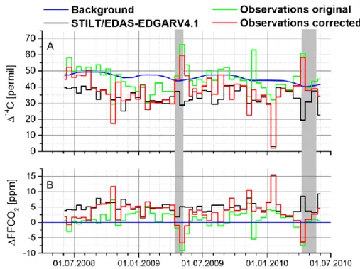
2 in Egbert (cf. Section 2.1) forms the basis for this assessment. In Figure 7A, the 14Cmeas data from Egbert do not consistently show the expected depletion patterns when compared to the background value. There are several situations when the 14Cmeas surpasses
14C
bg. This emphasizes the strong influence that nuclear power plant emissions have on this record. The modeled 14C using the STILT/EDAS-EDGARV4.1 framework shown in Figure 7 is derived by adding the modeled depletion due to the fossil fuel CO2 emissions (cf. Section 2.4) and 14Cbg. We find that 14C
meas deviates very strongly from this 14Cmod. As expected, when corrected with FFCO2,mask the agreement with 14Cmod is significantly improved. In addition, the general level as well as the seasonal pattern is met and there is strong improvement in the winter of 2009/2010. This clearly demonstrates the need to apply a nuclear industry correction at the Egbert site. Although a previous study by Graven and Gruber (2011) did unfortunately not have a suitable modeling framework, they already suggested that better resolved 14CO
2 emission data could improve our ability to correct for FFCO2,masked. Our high-resolution lagrangian modeling framework and
observations can now confirm this. The benefit of correcting the apparent FFCO2 (derived from the observations alone) with the modeled FFCO2,mask to retrieve the true FFCO2 is illustrated in Figure 7B. While the mean of the uncorrected observations (i.e. the apparent FFCO2) is 1.4 ppm (standard error 0.3 ppm) for the period from June 2008 to June 2010, the corrected average is 4.2 ± 0.6 ppm, which is close to the modeled FFCO2 of 5.1 ppm (standard error 0.3 ppm). The uncertainty estimate of ±0.6 ppm for the observed FFCO2 includes a 20% uncertainty for the 14CO2 correction and the standard error of the observations. Including the uncertainty of the biospheric 14CO2 correction did not significantly increase this uncertainty. The influence of erroneous atmospheric transport modelling on both FFCO2,mask as well as the modeled FFCO2 might be significant but is hard to quantify. For the modeled FFCO2, the standard error (i.e. 0.3 ppm) should only be regarded as the lower bound of the uncertainty. Peylin et al. (2011), for example, reported an uncertainty due to model transport for an ensemble of atmospheric transport models for an urban site near Costana, Romania, of 0.6 ppm for monthly averages. As our modeling framework is better resolved, we might expect this to be the upper bound of the transport model uncertainty. One could also expect that the transport model uncertainty is further decreased for long-term averages such as our 2-yr mean.
Figure 7 A) The modeled 14C data (including FFCO
2 emissions) in Egbert are given in black, the originally
observed data in green, the corrected observations in red and compared to the 14C of the Northern
Hemispheric background (i.e. Jungfraujoch). B.) FFCO2 derived from the 14C data (same color code).
Episodes of reported major maintenance at the nuclear power plants is given in gray (see text).
The observed and modeled FFCO2 data display similar long-term variations as well as sample-tosample variability. This data, however, is only included to illustrate the possible impact of failing to properly account for 14CO2 emissions, while a detailed discussion of the comparison of modeled
and observed FFCO2 is beyond the scope of this paper. The uncertainties of the means given are the standard error, with the data for 2 episodes in spring 2009 and 2010 (gray areas in Figure 7) being neglected. We find that the correction is not sufficient during these 2 episodes. The enhancement implies the correction is too small, thus suggesting even larger 14CO
2 emissions from the nuclear power plants during these periods. From the REMP report, we have learned that during these periods, extensive maintenance and reconstructions were performed at the Darlington NGS (15 April–3 May 2009) and Pickering NGS (15 April–24 May 2010). When assuming that the difference of our observed and modeled data is caused by enhanced emissions during these episodes, we can retrieve an emission estimate using STILT/EDAS. We find that during the maintenance episodes, the 14CO2 emissions are increased by a factor of 9 for the Darlington NGS and by a factor of 15 for the Pickering NGS, respectively.
The data from these 2 episodes are thus neglected in the quantitative assessment. Figure 8 shows that the raw observational 14C has only a weak correlation with the modeled 14C, with R = 0.39. The slope of 0.43 ± 0.15 and the large intercept of 30 ± 5‰ suggest that uncorrected 14C
meas can basically not be used to retrieve a reasonable estimate of FFCO2 at Egbert. The results when using the parameterized 14CO
2 emissions to correct 14Cmeas is given for comparison, but only show minor improvements. When using the CNSC emissions as the basis for the corrected 14Cmeas, the retrieved slope of 1.01 ± 0.14 is in agreement with a 1:1 line and shows that the corrected observations of 14C can be used to infer FFCO2. The corrected data have an improved correlation of R = 0.74 with the model results. The remaining variability of the data set is most likely caused by intra-annual variability of the 14CO
2 emissions from the CANDU power plants and an erroneous representation of atmospheric transport in the used model. Errors in the spatial distribution of the fossil fuel CO2 emission inventory in the Greater Toronto Area, which are known to be significant for other anthropogenic greenhouse gases (Vogel et al. 2012), may contribute as well. The small general offset of 2 ± 5‰ is statistically in agreement with zero, but could point towards a small underestimation of the contribution from local biospheric 14CO
2 fluxes or, as mentioned above, be due to the choice of our background.
Figure 8 Comparing the STILT-EDAS modeled atmospheric 14C to the observed 14C (green circles) and 14C after applying the nuclear power plant correction using
the parameterized emission model (gray triangles) and the CNSC emissions (red squares). The error bars denote the analytical precision for the observed 14
C and an additional 20% uncertainty of the 14
C correction for the CNSC-based correction. For clarity, no error bars are shown for the parameterized 14
C corrections, but they can span up to 1000% (see section 2.3).
SUMMARY AND CONCLUSION
This study aimed at assessing the implications of nuclear power plant 14CO
2 emissions on deriving FFCO2 estimates in a densely populated region that can be expected to be a hot spot of anthropogenic 14CO2 emissions (Graven and Gruber 2011). For this task, we used 3 data sets: 1) 10 yr (2000– 2011) of measured and officially reported 14CO2 emissions from the Canadian Nuclear Safety Committee (CNSC) and a parameterized 14CO2 emission inventory; 2) the results of our high-resolution modeling study (2006–2011); and 3) 2 yr (June 2008–June 2010) of observed atmospheric
14C at Egbert, Canada, as well as Northern Hemispheric background 14C.
The first step of comparing the parameterized emissions to the reported emission data uncovered that the assigned emission ratio of 1.6 TBq(GWa) 1 in the parameterization is in agreement with the measured average of all CANDU reactors of 1.50 ± 0.18 TBq(GWa) 1 as an overall mean. We could also quantify the emission ratio deviations using data from all Canadian CANDU reactors, which range from 0.65 ± 0.09 to 3.4 ± 0.82 TBq(GWa) 1. A parameterized inventory is, furthermore, not able to correctly describe the interannual variability of the (average) 14CO2 emissions, which have an interquartile range of 1.07 TBq(GWa) 1. Graven and Gruber (2011) reported large uncertainties and suggested that better resolved 14CO
2 emission data would be needed. Our study could show that using a parameterized approach is not suitable to derive 14CO
2 emissions in a hot spot region with multiple power plants and that regional studies should account for the different emission ratios of individual reactors. Ideally, the reactor-specific emission data should be compiled in future inventories and a parameterization-based approach be only used for regions that lack an official reporting.
To infer the influence of the different 14CO2 bottom-up emissions on the atmospheric 14CO2 levels, we conducted a pseudo-data experiment. From the modeled 14CO2 time series (2006–2011), we learned that using different 14CO2 emissions causes modeled 14CO2 to deviate significantly and the ratio of 14CO2,CNSC and 14CO2,para ranges from 0.5 to 2.0. To put this in perspective, the local depletion of 14C due to the addition of fossil fuel CO
2 was examined for our modeled time series from 2006 to 2011. We found that for the reported nuclear industry emissions, the annual average of the masked share accounts for 56% of FFCO2 and ranges from 27% in 2009 to 82% in 2007. This underlines the importance of a proper correction of the nuclear 14CO2 emissions in this region as it sometimes outweighs the actual signal we are after (i.e. the 14CO2 depletion due to FFCO2 emissions) even though our site is on the fringe of the most densely populated area of Canada. The simulation using the parameterized emissions is able to nearly reproduce the average annual value of masked FFCO2, yet the variability of 41–56% is severely underestimated. For our study period (2006– 2011), this translates into a spurious trend of about 30% in the calculated FFCO2. This might cause
a misinterpretation of either the temporal variations of the FFCO2 emissions or the spatial distribution of the FFCO2 sources, if they were used in an atmospheric inversion framework. We used our 2-yr-long observational time series from Egbert, Ontario, to assess if applying the CNSC reported 14CO2 emissions is sufficient to adequately model the local 14CO2 excess and thus FFCO2mask. The correlation of modeled and observed 14C is significantly improved from 0.39 to 0.74. Even more importantly, the slope of 14Cmod to 14Cobs changes to 1.01 ± 0.14 from previously 0.43 ± 0.15, thus permitting us to reliably estimate FFCO2 from the depletion in 14Cobs. The observed, apparent FFCO2 for our time period of 1.4 ± 0.4 ppm is corrected to 4.2 ± 0.6 ppm, which is close to the STILT/EDAS-EDGARV4.1 model result of 5.1 ± 0.3 ppm for this time series. One can expect that both biases and uncertainties in the FFCO2 fluxes as well as transport model biases and uncertainties contribute to the model-observation mismatch. Other studies have indicated that the greenhouse gas emissions of the Greater Toronto Area are overestimated in EDGARV4.1 (Vogel et al. 2012). The transport model error will affect both the modele d FFCO2 as well as the calculation of FFCO2,mask. Future studies aiming to quantify FFCO2 fluxes by interpreting the model-observation mismatch of individual samples rather than long-term averages will need to quantify the model transport error.
Although our applied 14CO2 correction seems sufficient on average, we find significantly elevated 14C values in individual biweekly integrated samples. This points towards a neglected intra-annual variability. Combining the observations with our high-resolution modeling framework we find that the 14CO
2 fluxes of specific nuclear power plants can increase by a factor of 9 to 15 during maintenance periods. As maintenance work has to be performed on a regular basis, e.g. every 5 yr, any long-term monitoring program will have to account for this. This type of emissions can be assumed to be intermittent and the area of influence for our observations can also change rapidly. Therefore, 14CO
2 emission data on daily or synoptic timescale would be desirable. This seems unrealistic at the moment, but weekly to monthly average 14CO2 emissions might be feasible for many sites and would decrease the uncertainty of FFCO2,mask and help to identify situations where the observational data needs to be flagged. Until these high-resolution emission inventories are available, data flagging might be an option for sites within hot spot regions (like Egbert), as the signal is noticeable in the observed 14C time series. Identifying such periods at sites further downwind of the nuclear power plant site will, however, be challenging. Although the effect will be smaller there, it, if not accounted for, can still cause a (significant) bias in the fossil fuel CO2 estimate. This is especially noteworthy as the highly populated regions e.g. the NE coast of America can be affected by CANDU and other nuclear reactors. Previous studies estimated that the emissions of the nuclear industry account for a masking of about 0.2–0.8 ppm FFCO2 (monthly average) for a site downwind of Ontario (Miller et al. 2012) or ratios of FFCO2,mask to FFCO2 of 0–90% (Graven and Gruber 2011). Our study suggests that the influence of Canadian CANDU reactors should be expected to be at the upper end of this range.
Although southern Ontario is a hot spot of nuclear 14CO2 emissions, the improvements achieved by incorporating the CNSC emission data is apparent and the level of agreement of the annual averages is quite promising. When including auxiliary tracers, such as CO or black carbon, future studies to infer FFCO2 fluxes appear to be viable. The transport model errors will then have to be addressed quantitatively by comparing different high-resolution transport models, which will also help to quantify the transport model uncertainty for different temporal aggregations. The long-term
perspective could be a network of multiple sites in this region that provides 14CO2 observations for a high-resolution inversion framework that allows to simultaneously estimate the release of 14CO2 by the nuclear industry and the regional FFCO2 emissions.
ACKNOWLEDGMENTS
The authors would like to thank Robert Kessler, Michele Ernst, and Lauriant Giroux for their diligent care and efforts for the 14CO2 sampling program of Environment Canada. We would especially like to thank Bernd Kromer and the staff of the 14C laboratory in Heidelberg for their careful work analyzing the 14CO2 samples. We also thank 2 anonymous reviewers for their comments and suggestions that helped to improve our manuscript. This work was supported by the Environment Canada Clean Air Regulatory Agenda (CARA) and funding received by FRV through a Visiting Fellowship to the Canadian Government Laboratories Award by the National Science and Engineering
Research Council of Canada (NSERC).
REFERENCES
Andres RJ, Boden TA, Breon FM, Ciais P, Davis S, Erickson D, Gregg JS, Jacobson A, Marland A, Mille r J, Oda T, Olivier JGJ, Raupach MR, Rayner P, Treanton K. 2012. A synthesis of carbon dioxid e emissions from fossil-fuel combustion. Biogesciences 9:1845– 71.
Beninson D, Gonzalez AJ. 1982. Application of the dose limitation system to the control of 14
C releases from heavy-water-moderated reactors. IAEA-SM-258/53. Dias C, Santos R, Stenström K, Nicoli I, Skog G, da
Silveira Corrêa R. 2008. 14
C content in vegetation in the vicinities of Brazilian nuclear power reactors.
Journal
of Environmental Radioactivity 99(7):1095–101.
Emission Database for Global Atmospheric Research [EDGAR]. Release version 4.1 of the European Commission, Joint Research Centre (JRC)/Netherlands Environmental Assessment
Agency (PBL). Available from
http://edgar.jrc.ec.europa.eu. Accessed 10 January 2011.
Gerbig C, Lin JC, Wofsy SC, Daube BC, Andrews AE, Stephens BB, Bakwin PS, Grainger CA. 2003. Toward constraining regional-scale fluxes of CO2
with atmospheric observations over a continent: 1. Observed spatial variability from airborne platforms.
Journal of Geophysical Research: Atmospheres
108:4756, doi: 10.1029/2002JD003018.
Guan D, Liu Z, Geng Y, Lindner S, Hubacek K. 2012. The gigatonne gap in China’s carbon dioxid e inventories. Nature Climate Change 2(9):672–5. Graven HD, Gruber N. 2011. Continental-scale
enrichment of atmospheric 14CO
2 from the nuclear
power industry: potential impact on the estimation of
fossil fuel-derived CO2. Atmospheric Chemistry and
Physics 11:12,339–49.
Graven HD, Guilderson TP, Keeling RF. 2012. Observations of radiocarbon CO2 at seven global
sampling sites in the Scripps flask network: analysis of spatial gradients and seasonal cycles. Journal of
Geophysical Research 117: D02303,
doi:10.1029/2011JD016535.
Hesshaimer V, Levin I. 2000. Revision of the stratospheric bomb 14CO
2 inventory. Journal of
Geophysical Research 105(D9):11,641– 58.
Holton JR, Haynes PH, McIntyre ME, Douglass AR, Rood BR, Pfister L. 1995. Stratosphere-troposphere exchange. Reviews of Geophysics 33(4):403–39. Hsueh DY, Krakauer NY, Randerson JT, Xu X,
Trumbore SE, Southon JR. 2007. Regional patterns of radiocarbon and fossil fuel-derived CO2 in surface air
across North America. Geophysical Research Letters 34: L02816, doi:10.1029/2006GL027032.
Kromer B, Münnich KO. 1992. CO2 gas proportional
counting in Radiocarbon dating—review and perspective. In: Taylor RE, Long A, Kra RS, editors.
Radiocarbon After Four Decades. New York:
Springer-Verlag. p 184–97.
Levin I, Münnich KO, Weiss W. 1980. The effect of anthropogenic CO2 and 14C sources on the distribution
of 14CO
2 in the atmosphere. Radiocarbon 22(2):379–
91.
Levin I, Naegler T, Kromer B, Diehl M, Francey RJ, Gomez-Pelae z AJ, Steele LP, Wagenbach D, Weller R, Worthy DEJ. 2010. Observations and modelling of the global distribution and long-term trend of atmospheric 14CO
2. Tellus B 62:26–46.
Levin I, Kromer B, Schmidt M, Sartorius H. 2003. A novel approach for independent budgeting of fossil fuel CO2 over Europe by
14
CO2 observations.
Geophysical Research Letters 30:2194, doi:10.1029/
Levin I, Rödenbeck C. 2008. Can the envisaged reductions of fossil fuel CO2 emissions be detected by
atmospheric observations? Naturwissenschaften 95(3): 203–8.
Lin JC, Gerbig C, Wofsy SC, Andrews AE, Daube BC, Davis KJ, Grainger CA. 2003. A near-field tool for simulating the upstream influence of atmospheric observations: the Stochastic Time-Inverted Lagrangian Transport (STILT) model. Journal of
Geophysical Research (Atmospheres) 108:4493,
doi:10.1029/ 2002JD003161.
Marland G, Hamal K, Jonas M. 2009. How uncertain are estimates of CO2 emissions? Journal of Industrial
Ecology 13:4–7.
Miller JB, Lehman SJ, Montzka SA, Sweeney C, Mille r BR, Wolak C, Dlugokencky EJ, Southon JR, Turnbull JC, Tans PP. 2012. Linking emissions of fossil fuel CO2 and other anthropogenic trace gases using
atmospheric 14CO
2. Journal of Geophysical Research
117: D08302, doi:10.1029/2011JD017048.
Naegler T, Levin I. 2009. Biosphere-atmosphere gross carbon exchange flux and the 13CO
2 and 14CO2
disequilibria constrained by the biospheric excess radiocarbon inventory. Journal of Geophysical
Research 114: D17303, doi:10.1029/2008JD011116.
Naegler T, Ciais P, Rodgers K, Levin I. 2006. Excess radiocarbon constraints on air-sea gas exchange and the uptake of CO2 by the oceans. Geophysical
Research Letters 33: L11802,
doi:10.1029/2005GL025408.
Nassar R, Napier-Linton L, Gurney KR, Andres RJ, Oda T, Vogel FR, Deng F. 2012. Improving the temporal and spatial distribution of CO2 emissions from global
fossil fuel emission datasets. Journal of Geophysical
Research: Atmospheres 118:917–33.
Peylin P, Houweling S, Krol MC, Karstens U, Pieterse G, Ciais P, Heimann M. 2011. Importance of fossil fuel emission uncertainties over Europe for CO2 modeling: model intercomparison. Atmospheric
Chemistry and Physics 11(13):6607– 22.
Rasch PJ, Tie X, Boville BA, Williamson DL. 1994. A three-dimensional transport model for the middle atmosphere. Journal of Geophysical Research 99(D1): 999–1017.
Radiological Environmental Assessment Progra m [REMP]. 2012. Available from http://www.opg.com/ news/reports/. Accessed 21 January 2012.
Robertson JAL. 1978. The CANDU reactor system: an appropriate technology. Science 199(4329):657–64. [StatsCan] Statistics Canada, Government of Canada. 2008. Census 2006 (Internet; cited 2011 October 4). Available from http://www40.statcan.gc.ca/. Stuiver M, Polach HA. 1977. Discussion: reporting of 14C data.
Radiocarbon 19(3):355–63.
Sweeney CE, Gloor E, Jacobson AR, Key RM, McKinley G, Sarmiento JL, Wanninkhof R. 2007.
Constraining global air-sea gas exchange for CO2 with
recent bomb 14
C measurements. Global
Biogeochemical Cycles 21: GB2015,
doi:10.1029/2006GB002784.
Trumbore SE. 2000. Age of soil organic matter and soil respiration: radiocarbon constraints on belowground C dynamics. Ecological Applications 10(2):399–411. Trumbore S. 2006. Carbon respired by terrestrial
ecosystems – recent progress and challenges. Global
Change Biology 12:141–53.
Turnbull JC, Miller JB, Lehman SJ, Tans PP, Sparks RJ, Southon J. 2006. Comparison of 14CO
2, CO, and SF6
as tracers for recently added fossil fuel CO2 in the
atmosphere and implications for biological CO2
exchange. Geophysical Research Letters 33: L01817, doi:10.1029/2005GL024213.
Turnbull JC, Miller JB, Lehman SJ, Hurst D, Peters W, Tans PP, Southon J, Montzka SA, Elkins JW, Mondeel DJ, Romashkin PA, Elansky N, Skorokhod A. 2009a. Spatial distribution of 14
CO2 across Eurasia:
measurements from the TROICA-8 expedition.
Atmospheric Chemistry and Physics 9(1):175–87.
Turnbull J, Rayner P, Miller JB, Naegler T, Ciais P, Cozic A. 2009b. On the use of 14CO
2 as a tracer for
fossil fuel CO2: quantifying uncertainties using an
atmospheric transport model. Journal of Geophysical
Research 114: D22302, doi:10.1029/2009JD012308.
United Nations Scientific Committee on the Effects of Atomic Radiation [UNSCEAR]. 1988, 1993, 2000. Sources and effects of ionizing radiation, UNSCEA R 1988, 1993, 2000 Report to the General Assembly. Vienna: UNSCEAR.
Vogel FR, Hammer S, Steinhof A, Kromer B, Levin I. 2010. Implication of weekly and diurnal 14
C calibration on hourly estimates of CO-based fossil fuel CO2 at a moderately polluted site in southwestern
Germany. Tellus B 62:512–20.
Vogel FR, Ishizawa M, Chan E, Chan D, Hammer S, Levin I, Worthy DEJ. 2012. Regional non-CO2
greenhouse gas fluxes inferred from atmospheric measurements in Ontario, Canada. Journal of
Integrative Environmental Sciences 9(Supplement
1):41–55.
Wanninkhof R. 1992. Relationship between wind speed and gas exchange over the ocean. Journal of
Geophysical Research 97(C5):7373–82.
Weiss R, Nisbet E. 2010. Top-down versus bottom-up.