HAL Id: hal-02477418
https://hal.archives-ouvertes.fr/hal-02477418
Submitted on 17 Feb 2020
HAL is a multi-disciplinary open access
archive for the deposit and dissemination of
sci-entific research documents, whether they are
pub-lished or not. The documents may come from
teaching and research institutions in France or
abroad, or from public or private research centers.
L’archive ouverte pluridisciplinaire HAL, est
destinée au dépôt et à la diffusion de documents
scientifiques de niveau recherche, publiés ou non,
émanant des établissements d’enseignement et de
recherche français ou étrangers, des laboratoires
publics ou privés.
diversity around Aldo Leopold’s shack in Baraboo,
Wisconsin, USA
Maryam Ghadiri Khanaposhtani, Amandine Gasc, Dante Francomano, Luis
Villanueva-Rivera, Jinha Jung, Michael Mossman, Bryan Pijanowski
To cite this version:
Maryam Ghadiri Khanaposhtani, Amandine Gasc, Dante Francomano, Luis Villanueva-Rivera, Jinha
Jung, et al.. Effects of highways on bird distribution and soundscape diversity around Aldo Leopold’s
shack in Baraboo, Wisconsin, USA. Landscape and Urban Planning, Elsevier, 2019, 192, pp.103666.
�10.1016/j.landurbplan.2019.103666�. �hal-02477418�
Contents lists available atScienceDirect
Landscape and Urban Planning
journal homepage:www.elsevier.com/locate/landurbplan
Research Paper
E
ffects of highways on bird distribution and soundscape diversity around
Aldo Leopold
’s shack in Baraboo, Wisconsin, USA
Maryam Ghadiri Khanaposhtani
a,⁎, Amandine Gasc
a,1, Dante Francomano
a,
Luis J. Villanueva-Rivera
a,2, Jinha Jung
a,3, Michael J. Mossman
b, Bryan C. Pijanowski
aaCenter for Global Soundscapes and Department of Forestry and Natural Resources, Purdue University, B066 Mann Hall, 203 South Martin Jischke Drive, West Lafayette,
IN 47907, USA
bWildlife and Forestry Research Section, Wisconsin Department of Natural Resources, 2801 Progress Road, Madison, WI 53716, USA
A R T I C L E I N F O Keywords: Bird community Traffic noise Road effect Soundscape LiDAR Habitat structure A B S T R A C T
In the 1940s, Aldo Leopold took extensive notes on birds and their sounds near his iconic shack in Baraboo, Wisconsin, USA. His observations, along with his land management techniques, helped frame his seminal book, A Sand County Almanac. After his death, two interstate highways were built near his property and subjected this historically significant area to traffic noise. While highways currently represent vital transportation corridors, their observed and potential impacts on biodiversity and ecosystem services are cause for concern. As the area including Leopold’s shack is now an Important Bird Area, we sought to evaluate the impact of these highways on the bird community and its related acoustic diversity. In 2011, 150 avian point counts were conducted in the three main habitats composing the landscape—upland deciduous forest, floodplain forest, and herbaceous wetland. In 2012, soundscape recordings were collected in sevenfloodplain forest sites using automated passive acoustic recorders. We described the local bird communities and measured their acoustic diversity. Linear models accounting for additional factors including land cover and vegetation structure characteristics showed that as the distance from highways increased, bird community descriptors (overall abundance and species richness) and acoustic diversity increased (when relationships were significant). On the species level, forest interior specialists were negatively affected by the presence of the highways, contrary to edge specialists. In addition to the direct effects of the edges produced by the highway structure, this difference might be due to the masking effect of traffic noise on interior specialists’ low-frequency vocalizations and their reliance on acoustic, as opposed to visual, communication. We conclude that while habitat structure is a principle driver of bird diversity on a broader scale, highway-induced changes in both habitat structure and soundscapes may affect bird communities.
1. Introduction
In the study of environmental ethics and wilderness conservation, one cannot overstate the impact of Aldo Leopold’s (1887–1948) work, as his naturalistic observations became a cornerstone of the conserva-tion biology movement and wildlife ecology (Burke, 2000; Callicott, 1990, 1999; Flader, 1994). Much of the observation and writing that critically shaped his ideas took place on his property in south-central Wisconsin where he authored his seminal book, A Sand County Almanac.
This groundbreaking work poetically describes the ethics, policies, and land management practices necessary to preserve ecological integrity while meeting human needs. Leopold observed that the soundscapes of his land were substantially influenced by bird populations (Bocast, 2013; Leopold, 1970), which are indicators of environmental health (Bocast, 2013; Gregory & van Strien, 2010). In the early 1960s, how-ever, Interstate 90 (I-90) and Wisconsin State Trunk Highway 78 (now I-39) were routed near this historically significant area, consequently changing its landscape and the corresponding soundscapes.
https://doi.org/10.1016/j.landurbplan.2019.103666
Received 6 June 2019; Received in revised form 8 September 2019; Accepted 9 September 2019
⁎Corresponding author at: Center for Community and Citizen Science, School of Education, University of California, Davis 1460 Drew Ave, Davis, CA 95618, USA.
E-mail addresses:mghadiri@ucdavis.edu(M. Ghadiri Khanaposhtani),amandine.gasc@ird.fr(A. Gasc),dfrancom@purdue.edu(D. Francomano),
villanueval@si.edu(L.J. Villanueva-Rivera),Jinha.Jung@tamucc.edu(J. Jung),mikemossman@wildblue.net(M.J. Mossman),
bpijanow@purdue.edu(B.C. Pijanowski).
1Present address: Aix Marseille Univ, Avignon Université, CNRS, IRD, IMBE, Marseille, France.
2Present address: Digitization Program Office, Smithsonian Institution, 600 Maryland Ave SW Ste 810W, Washington, DC, 20024-2520, USA. 3Present address: School of Engineering and Computer Sciences, Texas A&M University, 6300 Ocean Drive, Corpus Christi, TX 78412-5797, USA.
Available online 20 September 2019
0169-2046/ © 2019 Elsevier B.V. All rights reserved.
Ecosystem functions depend on structural characteristics, including vertical vegetation profiles (MacArthur & MacArthur, 1961) and plant species composition (James & Wamer, 1982), and road construction changes these structural characteristics, often resulting in biodiversity loss or novel species assemblages (Pimm, Russell, Gittleman, & Brooks, 1995; Vitousek, 1994). For forest birds in particular, structural char-acteristics determine habitat suitability (MacArthur & MacArthur, 1961; MacArthur, 1964) by providing foraging and nesting opportu-nities as well as suitable locations from which vocalizations will pro-pagate well (Farina & Belgrano, 2006; Pijanowski, Farina, Gage, Dumyahn, & Krause, 2011). More specifically, road networks affect bird
populations (Benítez-López, Alkemade, & Verweij, 2010; Habib, Bayne, & Boutin, 2007; Reijnen & Foppen, 2006) by physically fragmenting habitats and by generating traffic noise, which we define here as non-functional, unintentional, low-frequency sound (< 2 kHz) caused by on-road vehicles. Traffic noise can drastically affect avian commu-nication, as this frequency range overlaps with the frequency ranges in
which some bird species produce sound (Halfwerk, Holleman, Lessells, & Slabbekoorn, 2011). Such continuous anthropogenic noise disturbs complex animal social structures (Cartwright, Taylor, Wilson, & Chow-Fraser, 2014), as acoustic communication is vital for birds to find mates, defend territories, hunt, and navigate landscapes (Catchpole & Slater, 2003; Farina & Belgrano, 2006).
Acoustic communication occurs in the context of a soundscape—the total collection of all biological, geophysical, and technological sounds (biophony, geophony, and technophony, respectively) occurring at a given place over a given time period (Mullet, Gage, Morton, & Huettmann, 2016; Pijanowski, Farina, et al., 2011; Pijanowski, Villanueva-Rivera, et al., 2011; Qi, Gage, Joo, Napoletano, & Biswas, 2008). Birds and other animals have evolved to communicate e ffec-tively in the natural physical structure and biophonic and geophonic conditions of their habitats (Lengagne & Slater, 2002; Luther, 2009; Morton, 1975). Technophony represents a potential impediment to such communication, however, and soundscape studies can be used to
consider the propagation of anthropogenic noise and the interactions between biophony and technophony. Recently, soundscape analyses have also been used to quantify biodiversity and spatiotemporal eco-logical change (Dumyahn & Pijanowski, 2011b; Francis, Paritsis, Ortega, & Cruz, 2011; Parris & Schneider, 2009; Pieretti & Farina, 2013; Shannon et al., 2016; Sueur & Farina, 2015; Summers, Cunnington, & Fahrig, 2011). Some adverse impacts of roads on birds, including edge effects, population isolation, and road mortality have been well docu-mented (Barber et al., 2011; Barber, Crooks, & Fristrup, 2010; Forman & Alexander, 1998; Forman, 2003), although there has been insufficient research on how roads impact avian soundscape contributions (Duarte et al., 2015; Pieretti & Farina, 2013). In order to promote avian con-servation, it is important to understand the impact of roads on bird populations and the resulting soundscapes composed of traffic noise and altered bird sounds.
It is necessary to understand the sonic and non-sonic impacts of roads on bird communities in order to implement landscape-level conservation strategies to sustain bird communities (Francis, Ortega, & Cruz, 2011; Smith & Pijanowski, 2014). In this study, our objective was to evaluate the impact of two major highways (I-90 and I-39, hereafter referred to as“highways”), on the bird community in the Leopold-Pine Island Important Bird Area (LPIIBA). This impact was quantified through avian point counts and passive acoustic monitoring. This study was also intended to demonstrate the utility of soundscape studies in evaluating disturbance impacts. Birds are highly dependent on acoustic communication and monitoring the acoustic diversity of bird commu-nities is a valuable strategy to assess the consequences of sonic and non-sonic ecosystem disturbances. Furthermore, we sought to understand how other dominant landscape drivers affect bird distribution in a landscape of upland deciduous forest,floodplain forest, and herbaceous wetland at LPIIBA. To achieve these objectives, we 1) quantified the effect of distance from highways on the overall abundance, species richness, and composition of the bird community, 2) quantified the relative soundscape contributions of biophony, here dominated by bird sounds, and technophony, produced by highways in the study area, 3) investigated the effect of highways on avian acoustic diversity, and 4) examined the impact of other habitat structure variables on the bird community.
2. Methods
2.1. Study area
This study was conducted in the 6070-ha LPIIBA, located in Sauk and Columbia Counties of Wisconsin, along the Wisconsin River. The LPIIBA includes the Leopold Memorial Reserve (with the historic Aldo Leopold Shack), the Wisconsin Department of Natural Resources Pine Island Wildlife Area, and several private and federally owned tracts. This mixed forest-grassland-marsh landscape comprises three primary habitats: upland deciduous forest,floodplain forest (woody wetland), and emergent herbaceous wetland (Fig. 1;Leigel, 1982; Sauk County Report, 2001). The elevation ranges from 245 to 286 m above sea level, and much of the area is periodically flooded by the Wisconsin and Baraboo Rivers.
2.2. Avian point counts
A trained observer (MJM) conducted avian point counts at 150 sites in the upper LPIIBA, south of the Wisconsin River. Sites were evenly distributed along parallel transects, with transects and sites along transects placed 400 m apart. Point counts were performed during the breeding season (May to July) of 2011 during the hours of 0500 to 1000 (GMT -6) when many birds are usually acoustically active (Bibby, Burgess, & Hill, 1992; Díaz, 2006; Laiolo, 2002). For each single visit at each site, the species and number of birds seen or heard within a 200 m radius during a period of 5 min were recorded (Mossman, Steel, &
Swenson, 2009). Sites were visited only once to prioritize spatial re-presentation over temporal repetition. Point counts were not conducted on windy or rainy days. Sites closest to highways were surveyed on weekends and holidays to minimize the impact of traffic noise on bird detection. As many identified birds tend to maintain territories throughout the breeding season, territory change in response to daily variation in traffic noise—and any bias introduced by weekend/holiday sampling near the highways—was likely minimal and secondary to the bias that might have been introduced by impaired detection (Pieretti & Farina, 2013; Reijnen, Foppen, Braak, & Thissen, 1995).
2.3. Soundscape recordings
For soundscape analysis we focused exclusively onfloodplain forest due to its large spatial coverage and even distribution in the study area, the need to capture the soundscapes of replicate sites, and a limited number of recorders. We collected soundscape recordings from 7 sites infloodplain forest using automated digital acoustic recorders (Model SM2+; Wildlife Acoustics, Inc.; Maynard, MA, USA). The recording sites were located at different distances from highways (450 to 2000 m), providing varying exposure to traffic noise. Recording sites were separated by at least 100 m to ensure spatial independence. The recorders captured 30 s of audio at the top of each hour from 0500 to 1100 (GMT -6) every day between June 11th and June 22nd, 2012 (inclusive). This time frame captured dawn choruses and was con-temporaneous with the point counts of the previous year. We recorded in stereo at a sampling rate of 44.1 kHz using the uncompressed .wav file format. Given the time of day, we assumed that the recordings were dominated by bird sounds. Trained observers (MGK and AG) listened to each recording and coded the recordings according to weather condi-tion, recording quality, and intensity of bird sounds. Rainy and windy recordings, as well as recordings including cricket and frog sounds, were identified and removed from the analyses. We also excluded re-cordings from 0500 to 0600 because of the negligible bird activity during that time. The resultant data set contained 420 recordings.
2.4. Bird community descriptors
We determined four bird community descriptors: 1) total number of individuals (hereafter referred to as“overall abundance”), 2) number of species (hereafter referred to as“species richness”), 3) species assem-blage (the identities of the species; hereafter referred to as“community composition”), and 4) acoustic diversity. The first three descriptors were quantified for each point-count site, and the last was quantified for each acoustic recording site. For community composition, only the presence/absence of each species was considered. FollowingJulliard, Jiguet, and Couvet (2004), we focused exclusively on common bird species with a total abundance of more than three individuals observed throughout the study area to avoid“incidental observations” (Murray et al., 2017). Accordingly, we considered only 46 of the 54 species observed (Appendix A). Interspecies differences in detectability through point counts can affect the estimation of “real” community descriptor values. Assuming that this bias is consistent throughout the study area, however, we consider“observed” community descriptor values as suf-ficient to evaluate the effects of the highways on the bird community. The acoustic production of a bird community reflects its diversity, behaviors, and abundance (Gasc, Pavoine, Lellouch, Grandcolas, & Sueur, 2015). Acoustic diversity was measured through 5 com-plementary acoustic indices calculated on each recording: the Acoustic Diversity Index (ADI) (Villanueva-Rivera, Pijanowski, Doucette, & Pekin, 2011), the Acoustic Complexity Index (ACI) (Pieretti & Farina, 2013), the Number of Frequency Peaks (NP) (Gasc, Sueur, Pavoine, Pellens, & Grandcolas, 2013), the Bioacoustic Index (BI) (Boelman, Asner, Hart, & Martin, 2007), and the Acoustic Occupancy Index (AOI). Audiofile manipulation and acoustic index calculation were performed using R (Team, 2016) and the packages “tuneR” (Ligges, 2013),
“soundecology” (Villanueva-Rivera, Pijanowski, & Villanueva-Rivera, 2016), and“seewave” (Sueur, Aubin, & Simonis, 2008).
The ADI reflects the Shannon diversity of 1-kHz frequency bins based on their associated amplitudes above a threshold of−50 dBFS. The ACI increases with variation in amplitude and frequencies, and it has been shown to be sensitive to the acoustic activity of bird com-munities (Farina, Pieretti, & Piccioli, 2011), which exhibit substantial frequency modulation. The temporal step for the ACI calculation was fixed at 5 s. The NP reflects the number of spectral peaks in a recording. As the number of bird species increases, the probability of new fre-quencies occurring in the soundscape increases. Consequently, the NP is expected to increase with the number of bird species, but it is also sensitive to bird species identity; its variation will depend on the community assemblage. The NP function employed a relative amplitude selection value of 0.01 and a frequency discrimination value of 200 Hz. The BI represents “the area under the frequency spectrum and above the minimum amplitude of the spectrum” and typically increases with overall abundance and species richness (Gasc, Francomano, Dunning, & Pijanowski, 2016). The AOI is defined as the number of Short Term Fourier Transform (STFT) windows associated with a relative amplitude above−50 dBA in any frequency bin. This index reflects the occupancy of acoustic space as defined by time and frequency. The AOI is equal to 1 when constant sound occurs at all frequencies. To avoid the biasing influence of traffic noise on these indices and to focus on bird sounds, only frequencies between 2 and 10 kHz were considered. Indices based on a STFT calculation used an STFT window size of 512 samples.
In addition, to evaluate the level of traffic noise across the area, we used the Normalized Difference Soundscape Index (Kasten, Gage, Fox, & Joo, 2012). The NDSI quantifies the relative soundscape contribu-tions of biophony, here dominated by bird sounds, and technophony, here dominated by traffic noise. The biophony range for the NDSI was defined as 2 to 10 kHz, while the technophony range was defined as 1 to 2 kHz. Possible index values range from−1 to 1, where negative values indicate a soundscape dominated by technophony and positive values indicate a soundscape dominated by biophony.
2.5. High priority species
The LPIIBA Strategic Vision (Mossman et al., 2009) identified sev-eral high-priority bird species that are, “considered of conservation priority due to declining [breeding] populations in the state or else-where in their range, declining or vulnerable habitats, specialized ha-bitat requirements, or some combination of these”. These species were also selected because they are good candidates to inform management decisions due to their well-documented habitat associations and their ability to serve as indicators of desirable plant-animal communities in the LPIIBA, (Mossman et al., 2009, P. 7). The high-priority species we found in the study area werefield sparrow (Spizella pusilla), marsh wren (Cistothorus palustris), sandhill crane (Antigone canadensis), swamp sparrow (Melospiza georgiana), and willowflycatcher (Empidonax traillii; Appendix A).
2.6. Land cover and vertical structure
Spatial and structural characteristics of the mixed landscape of the study area were calculated using the Geographic Information System (GIS) ArcMap (10.5.1). Data from Light Detection and Ranging (LiDAR) and the National Land Cover Database (NLCD 2011) were used to map land cover of the study area. For greater precision regarding this study area, we refer to the NLCD’s “woody wetland” class as “floodplain forest”. This classification also includes shrub swamp and areas that are shrubby marshes. Distance from highways and distance from rivers were extracted from other GIS layers (U.S. Major Highways (Streets dataset) and NHDF lowline (National Hydrology Database)). Discrete-return airborne LiDAR that partially covered the study area was ac-quired in May 2005 and the area did not exhibit noticeable changes in
habitat structure during the seven-year period between the LiDAR survey and acoustic recording (Mossman, personal communication, December 4, 2017). The partial LiDAR coverage forced us to limit the number of point count sites to 32 for use in further analysis considering the relationship of spatial and structural variables with acoustic indices. The LiDAR point cloud data were processed at 65-ft (19.812-m) spatial resolution so that each pixel used 183 points to generate a vertical profile. The following vertical structural characteristics of the vegetation were then extracted from the vertical profile as described by
Pekin, Jung, Villanueva-Rivera, Pijanowski, and Ahumada (2012) and Jung, Pekin, and Pijanowski (2013): 1) relative heights
(RHs)—eleva-tion above ground of the corresponding energy percentile in the vertical profile (e.g., RH100 is maximum canopy height and RH25 is height of 25% of the canopy), 2) canopy cover (CC)—intensity sum of all non-ground points divided by intensity sum of all points, 3) number of strata (NOS)—number of clusters in the vertical profile, and 4) vertical gap index (VGI)—total distance between individual canopy strata (empty vertical space) divided by RH100 (see Appendix B for the full list of variables and Appendix C for LiDAR metric details). Each point count and acoustic recorder site was associated with the variables from the pixel in which it was located.
The LiDAR data were also used to generate an open space layer, defined as areas with RH100 < 2 m (Brokaw, 1982). RH100 para-meters can be calculated with a smaller number of LiDAR points within each pixel, and an additional RH100 layer was generated at 10-ft spatial resolution from the LiDAR data. The 10-ft RH100 layer was then used to generate the open space raster layer at ft spatial resolution. This 10-ft RH100 layer was used instead of the 65-10-ft RH100 layer in all statis-tical analyses. The open space raster layer was processed to remove small patches by applying a 3x3filter and then coding the raster to a binary layer (0 = patches with area < 10 000 m2; 1 = patches with area > 10 000 m2). The resulting open space raster layer called“large
open space” was then converted to a polygon layer for further analysis. Afterward, the distance of each site from the closest open space (Dis_OS) and the area of that open space (Area_OS) were quantified. To determine the proportion of open space around each point-count and acoustic recorder site, the number of open space cells within a 10-m buffer of the site were divided by the total number of cells within the buffer. It was labeled “B10”. We performed the above calculations for all 7 acoustic recorder sites and the 32 bird survey sites that were within LiDAR coverage.
2.7. Statistical analysis
To evaluate the effects of distance from highways on overall abundance and species richness in upland deciduous forest,floodplain forest, and emergent herbaceous wetland (n = 29, 79, and 42, respec-tively), we employed separate linear regression models for each habitat type and dependent variable using the R package“car” (6 models; (Fox, 2002)). We also conducted separate analyses of similarities (ANOSIMs) for each habitat type to test for differences in community composition between binned distances from highways (using the R package vegan;
Oksanen, 2016). Forfloodplain forest, we calculated separate multiple linear regression models treating overall abundance, species richness, and each acoustic index as the dependent variable and distance from highways, distance from river, and habitat structure variables as in-dependent variables. Further details regarding these tests are described below.
In order to examine the impact of a road on community descriptors, it is important to identify the relevant range of distances over which such an impact can be observed (Alkemade et al., 2009). In order tofind the appropriate spatial scale or“effect-distance” (Reijnen & Foppen, 2006) at which to evaluate changes in descriptors, the relationships between descriptors (richness and abundance) and distance from highways were quantified within different buffer distances in 500-m increments. For this test, all point-count sites were considered because
they were widely distributed across a range of distances from highways (varying from 60 m to 4000 m). Linear regression models of bird di-versity indices as functions of distance from highways were applied based on data within the following buffer distances: 0 to 500, 0 to 1000, 0 to 1500, 0 to 2000, 0 to 2500, 0 to 3000, 0 to 3500, and 0 to 4000 m. F-statistics increased with increasing buffer distance and reached a maximum at 0 to 2000 m before decreasing (Fig. 2). Given this result, analyses were performed only on data within a buffer distance of 2000 m from highways.
For each of the linear regression models employed, the following model assumptions were verified: 1) independence of observations, 2) non-multicollinearity of independent variables, and 3) hetero-scedasticity, linearity, and normality of residuals. To avoid multi-col-linearity effects among independent variables in the multiple linear regression models, variance inflation factors were calculated using the R package “car” (Fox, 2002). Variables with a variance inflation
factor > 2 were excluded from the models. These excluded variables were RH100, RH75, RH50, CC, and Area_OS, and remaining variables were Dis_HWY, VGI, NOS, B10, Dis_Riv and Dis_OS. Linearity, hetero-scedasticity, and normality of residuals were graphically evaluated using scatterplot, bptest, and qq-plot, respectively (from the R package “lmtest” (Zeileis & Hothorn, 2002).
To investigate the variation of bird community composition with the distance from highways, sites were grouped into four distance ranges (0 to 500, 500 to 1000, 1000 to 1500, and 1500 to 2000 m), and differences were tested by an ANOSIM with 1000 permutations using the R package“vegan” (Oksanen, 2016).
As many acoustic observations (5 recordings per day over 12 days) were collected for each acoustic recording site in floodplain forest (n = 7), acoustic index values were averaged within each site to ensure the independence of these values. For each multiple linear regression model, we conducted backward stepwise regression analysis (stepAIC) using the R package“MASS” (Venables & Ripley, 2013). The best model
was selected using the Akaike Information Criterion (Akaike, 1981), where the best model had the lowest AIC and all models within ΔAIC < 2 were acceptable.
3. Results
The overall abundance per point-count site ranged between 6 and 31 with a mean of 16.10 and a standard error of 0.36 throughout the study area. Species richness ranged between 2 and 20 with a mean of 10.81 and a standard error of 0.26. Among the 46 common bird species considered in the analyses, song sparrows (Melospiza melodia), common yellowthroats (Geothlypis trichas), yellow warblers (Setophaga petechia), and red-winged blackbirds (Agelaius phoeniceus) were the most abun-dant, with study-area-wide per-species abundances of 226, 150, 134, and 129, respectively.
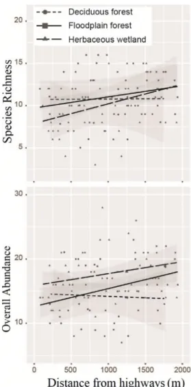
The relationships of species richness and overall abundance with distance from highways varied for each habitat (Fig. 3). In upland forests, the results did not show significant relationships. In floodplain forest, only abundance increased significantly with distance from highways (p-value = 0.01, r2= 0.11, standardized beta = 0.35), while in herbaceous wetland, only richness increased significantly with dis-tance from highways (p-value = 0.03, r2= 0.09, standardized
beta = 0.23).
The regression models associated with the lowest AIC values in-dicated that the drivers of overall abundance and species richness in floodplain forest were: 1) distance from highways, 2) vegetation gaps, and 3) number of strata, 4) proportion of open area within a 10-m buffer, and 5) distance from river. Considering the overall abundance, three models were equal, and considering the species richness two models were selected according to AIC. The linear regression models for overall abundance and species richness are presented inTable 1.
The ANOSIM results showed that bird community composition did not significantly change at different distances from highways in the
Fig. 2. F-statistics for regressions on bird abundance and richness as functions of distance from highways (relative to the highest F-statistic). Separate regressions were run using various distance limits ranging from 500 to 4000 m from highways. Empty circles represent non-significant relationships, while the full circles represent significant relationships. The dashed line shows the distance limit with the highest F-statistic.
upland deciduous forest and floodplain forest, but composition was significantly different in emergent herbaceous wetland (p-value = 0.02, r2= 0.12). While community composition was largely unchanged,
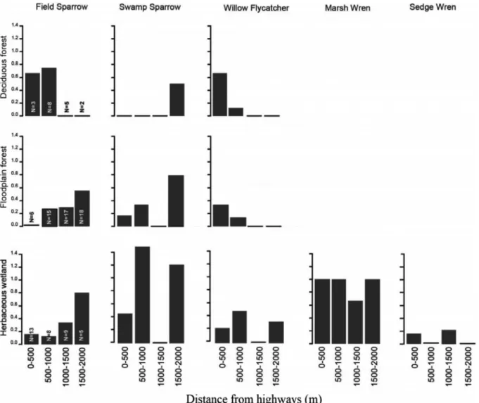
highway impacts differed by species, especially for per-species abun-dance.Fig. 4shows the response of some priority species at different distances from highways within each habitat. Some species such asfield sparrow (Spizella pusilla) were present in all three habitats, and their abundance increased with distance from highways within floodplain forest and emergent herbaceous wetland. Marsh wrens (Cistothorus palustris) were present only in herbaceous wetland, and their abun-dance was not affected by distance from highways (Fig. 4).
Among all 6 acoustic indices, the multiple linear regression models of the ADI, the NDSI, and the AOI were significant based on full model p-values (seeTable 2). Additionally, the ADI, the NDSI, and the AOI significantly increased with distance from highways (Fig. 5). The other indices with non-significant full-model p-values did not show any no-table trends in response to distance from highways. The significant models are presented inTable 2.
4. Discussion
The concept of biological diversity is multi-dimensional (Petchey & Gaston, 2002), and it is possible to generate different bird community
descriptors. Recent research supports the idea of considering acoustic diversity not only as an indicator of classical diversity—such as overall abundance or species richness—but also as another unique and separate
component of biological diversity (Gasc et al., 2016; Gasc et al., 2015; Lomolino, Pijanowski, & Gasc, 2015; Smith & Pijanowski, 2014; Sueur et al., 2008). Accordingly, we used data collected through avian point counts and passive acoustic monitoring to capture multiple bird com-munity descriptors. Our results support the concept that these two as-pects of biodiversity are complementary. Analyzed together, they pro-vide enhanced perspective for ecologists to understand disturbance impacts—particularly those involving noise. The impact of a major highway is twofold:first, its existence fragments habitats, creates edges, and changes landscape structure; second, noise from its traffic propa-gates far beyond its physical borders, potentially interfering with an-imal communication.
4.1. The influence of habitat structure
Many studies have highlighted the effects of habitat structure on the distribution of avian communities (James & Wamer, 1982; Karr & Roth, 1971; MacArthur & MacArthur, 1961) as well as the evolution of avian sounds (Boncoraglio & Saino, 2007; Morton, 1975). In thefloodplain forest component of our study, the result of multiple linear regression using distance from highways, distance from river, and LiDAR data to predict bird community descriptors revealed that the number of strata (representing structural complexity) was the sole significant contributor to changes in species richness. The number of strata has been shown to positively affect bird diversity by increasing feeding and nesting op-portunities, resulting in increased abundance and richness (Berg et al., 1994; Ghadiri Khanaposhtani, Kaboli, Karami, & Etemad, 2012; MacArthur & MacArthur, 1961). Distance from river was not a sig-nificant predictor in any regression model related to overall abundance, species richness, and community composition although it was sig-nificant in regression models for some acoustic indices. Research has shown how forest riparian zones can support bird communities with high-quality habitat created by the water-land ecotone and plant composition (Larue, Bélanger, & Huot, 1995; Nilsson & Dynesius, 1994), but ourfindings are consistent with studies such as those by
Whitaker and Montevecchi (1997) and Murray and Stauffer (1995)that revealed no differences in bird richness and abundance between in-terior forest and riparian habitats.
Fig. 3. The impact of distance from highways on overall abundance and species richness in three habitats within 2000 m of highways.
Table 1
Multiple linear regression models with the lowest Akaike information criteria (ΔAIC < 2) for bird abundance and richness in floodplain forest. Letters A and B indicate distinct models withΔAIC < 2.
Overall abundance Species richness
A B A B AIC 188.19 188.66 164.99 166.23 R2 0.26 0.24 0.22 0.20 p-value < 0.01** 0.01* 0.02* 0.04* Dis_HWY β = 0.47 p < 0.01** β = 0.39 p = 0.02* β = 0.21 p = 0.14 β = 0.25 p = 0.57 VGI – – β = 0.24 p = 0.15 β = 0.25 p = 0.15 NOS β = 0.21 p = 0.17 β = 0.22 p = 0.14 β = 0.30 p = 0.03* β = 0.38 p = 0.02* B10 – β = 0.21 p = 0.20 – – Dis_Riv – – β = 0.24 p = 0.09 –
* Significant at 0.05 level. ** Significant at 0.01 level.
Fig. 4. The impact of distance from highways on the average number of high-priority species per site in different habitats. N shows the number of sites per habitat within each range of distances from highways. Priority species with no notable response are not presented in thisfigure.
Table 2
Multiple linear regression models with the lowest Akaike information criteria (AICs) for acoustic indices infloodplain forest.
ADI NDSI AO BI ACI NP
AIC 23.01 10.32 48.25 14.82 40.02 15.55 R2 0.89 0.87 0.89 0.55 0.55 0.33 PValue 0.01* 0.03* < 0.01** 0.06 0.08 0.06 Dis_HWY β = 0.74 p < 0.01** β = 0.85p < 0.01** β = 0.78p < 0.01** β = −0.35p = 0.12 – – VGI β = −0.55 p < 0.01** β = −0.39 p = 0.09 β = −0.54 p < 0.01** β = −0.48 p = 0.06 β = −0.22 p = 0.06 β = −0.57 p = 0.08 NOS β = 0.35 p = 0.02* β = 0.35 p = 0.21 β = 0.49 p < 0.01** – – – Dis_OS – – – – – β = 0.53 p = 0.03* Dis_Riv β = −0.38 p = 0.03* β = 0.38 p = 0.16 β = −0.30 p = 0.01* β = −0.50 p = 0.06 β = −0.25 p = 0.02* –
* Significant at 0.05 level. ** Significant at 0.01 level.
4.2. The influence of the highways
In addition to the impact of habitat structure on species richness, we identified that distance from highways affects overall abundance and species richness, generally shifting the bird distribution away from highways. Infloodplain forest, overall abundance increased with dis-tance from highways, but species richness and community composition were relatively constant. In herbaceous wetland, overall abundance was relatively constant, species richness increased, and community com-position changed significantly with distance from highways. Among the three main habitats in the study area, upland deciduous forest was not
well represented as it was mainly distributed around highways. Its limited distribution could be a possible explanation for the non-sig-nificant change in overall abundance and species richness in that ha-bitat at different distances from highways. Notable increases in species abundances for interior species such as white-breasted nuthatch (Sitta carolinensis) and great-crestedflycatcher (Myiarchus crinitus) with in-creasing distance from highways infloodplain forest highlight some of the impacts of highways on community composition. These results support those of other studies that have demonstrated negative impacts of roads on bird abundance and richness (Benítez-López et al., 2010; Habib et al., 2007; Reijnen, Foppen, & Meeuwsen, 1996; Wiącek, Polak,
Fig. 5. Scatterplot of acoustic index values as a function of distance from highways. Grey points show all index values per site while the mean values and standard deviations are shown by red points and error bars. The dashed line in all images shows the linear regressionfitted to the data. (For interpretation of the references to color in thisfigure legend, the reader is referred to the web version of this article.)
Kucharczyk, & Bohatkiewicz, 2015). On the other hand, according to
Fretwell (1972) and Van Horne (1983), density of bird populations may not indicate habitat quality, as density can be high even in low-quality areas. Studies such as those byClavero, Villero, and Brotons (2011) and Devictor, Julliard, Couvet, and Jiguet (2008) highlighted the in-efficiency of metrics such as abundance and richness in showing the impact of disturbances on a bird community, and they support the use of community composition metrics. However, in our study, bird com-position did not show any change infloodplain forest related to dis-tance from highways, perhaps due to our use of presence/absence data and the elimination of uncommon species in our calculations.
Specialist bird species observed in this study were classified as in-terior or edge specialists based on previous studies and observed re-sponses to the physical and acoustic changes caused by highways. These two groups differ in their habitat structure preferences, reliance on acoustic communication, and evolutionary acoustic adaptations.
Forest interior specialists avoid edges and prefer complex vegetation structure because of the plant composition, the greater availability of tree holes, and the possible abundance of arthropods (Ghadiri Khanaposhtani et al., 2012; Laiolo, 2002; Villard, 1998; Villard, Schmiegelow, & Trzcinski, 2007). Interior specialists rely primarily on sound to communicate, given restrictions on visual communication due to dense vegetation structure (Farina & Belgrano, 2006; Goodwin & Shriver, 2011; Morton, 1975). The sounds of interior species tend to propagate well in structurally dense habitats. These species generally produce low-frequency sounds with limited frequency ranges to mini-mize medium absorption and reflective scattering, promoting effective communication within a densely structured environment (Boncoraglio & Saino, 2007; Goodwin & Shriver, 2011; Morton, 1975). Interior specialists are negatively affected not only by the physical changes caused by highways, but also by the masking effect of low-frequency noise from highways that can impair their communication by over-lapping with the frequencies those species produce (Dumyahn & Pijanowski, 2011a; Habib et al., 2007; Krause, 1987; Pijanowski, Villanueva-Rivera et al., 2011; Reijnen et al., 1995; Rheindt, 2003).
Conversely, edge specialists are attracted to roads, as they prefer open structure with a rich understory full of shrubs and young trees. Edges create a microhabitat where nesting opportunities and certain foods are available (Laiolo, 2002; Warner, 1992). These species, such as red-winged blackbird (Agelaius phoeniceus) and gray catbird (Dumetella carolinensis) live in shrubs and open countryside and are common along roads. These edge specialist species tend to produce higher-frequency sounds (Dowling, Luther, & Marra, 2011; Francis et al., 2011; Hu & Cardoso, 2009; Nemeth & Brumm, 2009) and utilize visual display as well as acoustic communication to attract mates. Therefore, they may be less sensitive to the impacts of traffic noise, and they may benefit from the suitable habitat conditions created by the presence of high-ways.
Bird species can evolve adaptations based on the properties of acoustic propagation throughout their range of habitats, and in-dividuals can modify behavior based on the active soundscapes in their specific habitats. The Acoustic Adaptation Hypothesis (AAH) refers to the evolution of bird sounds to maximize thefidelity of signal trans-mission through specific habitat structure (Boncoraglio & Saino, 2007; Job, Kohler, & Gill, 2016; Morton, 1975). Bird sounds are shaped ac-cording to structure-induced absorption and reflection, the amplitude and masking effects of natural ambient noise (e.g., wind and flowing water), and the hearing sensitivity of the intended receiver (Farina & Pieretti, 2014; Morton, 1975; Pekin et al., 2012). In a shorter temporal context, we use the Acoustic Plasticity Hypothesis (APH) to refer to the short-term behavioral responses to rapidly introduced noise that some bird species employ to mitigate the deleterious effects of noise on communication, predator detection, territory defense, and mating (Kociolek, Clevenger, St Clair, & Proppe, 2011; Slabbekoorn & Ripmeester, 2008). APH strategies include producing sound earlier in the morning, changing frequency, increasing amplitude, or repeating
the high-frequency parts of sounds to improve acoustic communication (Francis et al., 2011; Kociolek et al., 2011). Overall,“the element of time” (Morton, 1975) is a limiting factor in the evolution of sound production based on the AAH, but over long time scales, changes can be substantial. Behavioral adaptations based on the APH are achievable in the short term, but they are limited by current physiological restrictions on sound production. Studies have suggested that many birds have failed to behaviorally adapt to the interference of anthropogenic noise in their immediate environments (Rheindt, 2003), and the suscept-ibility of interior species to noise reflects their insufficient adaptation to date.
4.3. Soundscape impacts
In this study, 6 acoustic indices were used to analyze the impact of highways on soundscape diversity, and the results of the multiple linear regression models showed that only the ADI, the AOI, and the NDSI were significantly related to distance from highways in floodplain forest. Studies using acoustic indices have shown varying levels of correspondence with ecological hypotheses, and the indices may be subject to bias from varying ecosystem conditions that affect sounds-capes (Fuller, Axel, Tucker, & Gage, 2015; Machado, Aguiar, & Jones, 2017). Additionally, much work is still necessary to define ecosystem-specific sampling durations that will appropriately incorporate or minimize temporal soundscape variability to best address a given re-search question.Fuller et al. (2015)identified the ADI as a good in-dicator of dawn and dusk choruses and the NDSI as a good index for connecting“landscape characteristics to ecological condition and bird species richness”.Pieretti and Farina (2013)used the ACI to show the effect of traffic noise on the bird community in an oak woodland ha-bitat, and the results of their study indicate greater bird activity farther from the road, supporting our conclusions. In our results, the increase in the NDSI represents the increased ratio of biophony to technophony farther from the highway. The fact that this index takes inputs from two frequency ranges means that variation in either range could impact the index value. With increased distance from highways, the intensity of traffic noise (in the lower frequency range) decreases, and this could explain the variation in the NDSI (Machado et al., 2017). However, the results of the ADI indicate that the decrease in traffic noise was not the sole explanation for the increase in the NDSI. The ADI, which represents an acoustic version of the Shannon Index, had a threshold set to con-sider sound only above 2 kHz (which excluded most traffic noise). The fact that this index also increased with distance from highways means that bird acoustic activity did in fact increase, and also contributed to the increase in the NDSI. According to the Acoustic Habitat Hypothesis, which states that habitat selection behavior is based on habitat soundscapes (Mullet et al., 2016; Mullet, Farina, & Gage, 2017) birds might tend to live farther from noise sources like roads to avoid acoustic masking.
Several studies have shown that the edge effect on bird communities in forest ecosystems extends about 150 m from the road (Ortega & Capen, 2002).Forman and Deblinger (2000)quantified the width of the road-effect zone in a forest around a highway as up to 600 m, defining it as,“the area over which significant ecological effects [on species, soil, and water] extend outward from a road”. The road-effect zone is as-sociated with vehicular traffic and highly dependent on the structural and spatial composition of an ecosystem (Forman & Deblinger, 2000; Forman, 2000).Benítez-López et al. (2010), offered a larger estimate for the effect zone of traffic noise by asserting that it can affect bird communities up to 2600 m from a road. The bird survey sites in our study area were an average distance of 1300 m from highways, and despite the attenuation and absorption of the traffic noise by vegetation structure, low frequency noise from highways could be heard even at the farthest sites from the highways (1785 m) (Fig. 6). As our closest acoustic monitoring site was 466 m from a highway, the acoustic effects we observed occurred beyond the edge effect range indicated byOrtega
and Capen (2002) and beyond the range of most non-acoustic road
effects described byForman and Deblinger (2000). We can thus infer that the continued reduction in avian acoustic activity at greater dis-tances from highways could be primarily due to the impacts of traffic noise.
As management programs attempt to strategically prioritize their efforts, it is important to identify dominant drivers of biodiversity and their effects on animal communities in different ecosystems. In this study in the Leopold-Pine Island Important Bird Area, the effect of structural characteristics of thefloodplain forest on bird diversity was relevant, but highways also had significant effects on both overall abundance and acoustic diversity of the bird community. Across habitat types, the observed increases in overall abundance, species richness, and acoustic diversity with increased distance from highways probably result from physical edge effects and the masking effects of traffic noise, particularly for interior specialists. For species that cannot behaviorally adapt their acoustic communication to avoid these masking effects, sites farther from highways represent superior habitats. Our study ex-amined multiple aspects of diversity using different methodologies to more robustly understand the impact of highways on the local bird community, and more broadly, it supports the use of multifaceted biodiversity monitoring approaches to assess disturbance impacts.
Acknowledgments
This research was supported in part by computational resources provided by Rosen Center for Advanced Computation (RCAC) within Information Technology at Purdue University (ITAP). We thank the LPIIBA partners and especially the Aldo Leopold Foundation (ALF) for supporting IBA bird surveys and allowing audio data collection on ALF property. We also would like to thank John Dunning, Jeffrey Holland, Garett Pignotti, Brigid Manninghamilton, Mysha Clarke, Kristen Bellisario, Iman Beheshti Tabar, and Charles R. Wineland for their helpful comments on earlier drafts of this manuscript. The authors take all responsibility for accuracy and interpretation.
Appendix A. List of bird species recorded in point counts
Common name Scientific name Relative abundance
Sandhill crane†× Antigone canadensis 12◦
Mourning dove Zenaida macroura 37+
Northernflicker Colaptes auratus 14+
Red-bellied woodpecker Melanerpes carolinus 18+
Yellow-bellied sapsucker Sphyrapicus varius 8◦
Downy woodpecker Picoides pubescens 32+
Hairy woodpecker Picoides villosus 14+
Eastern wood-pewee Contopus virens 107+
Willowflycatcher† Empidonax traillii 20−
Great crestedflycatcher Myiarchus crinitus 67+
Yellow-throated vireo Vireoflavifrons 40+
Red-eyed vireo Vireo olivaceus 41+
Warbling vireo Vireo gilvus 51−
Blue jay Cyanocitta cristata 50+
American crow Corvus brachyrhynchos 11+
Tree swallow Tachycineta bicolor 17−
Tufted titmouse Baeolophus bicolor 15+
Black-capped chickadee Poecile atricapillus 55+
White-breasted nuthatch Sitta carolinensis 41+
House wren Troglodytes aedon 110+
Marsh wren† Cistothorus palustris 34−
Blue-gray gnatcatcher Polioptila caerulea 62+
Veery Catharus fuscescens 21−
Wood thrush Hylocichla mustelina 40−
American robin Turdus migratorius 120+
Gray catbird Dumetella carolinensis 87−
Cedar waxwing Bombycilla cedrorum 26−
Blue-winged warbler Vermivora cyanoptera 8−
Yellow warbler Setophaga petechia 134
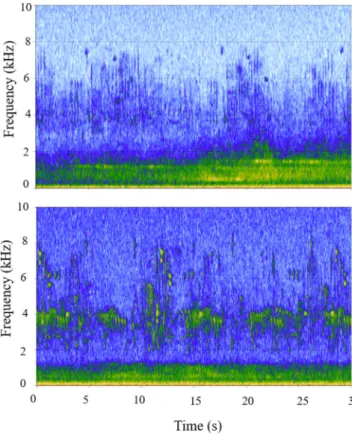
Fig. 6. Two spectrograms of 30-s soundscape recordings at 0600 h from July 1st
2012 in the LPIIBA. The top recording was made at 466 m from the highway, while the bottom recording was made at 1785 m from the highway. The bright color in lower frequencies (< 2 kHz) is due to traffic noise that exists at both sites. The intensity of the noise is higher at the site closer to the highway, while the frequency bands dominated by bird activity (2 to 8 kHz) are more active at the site farther from the highway.
Ovenbird Seiurus aurocapilla 48◦
Common yellowthroat Geothlypis trichas 150−
American redstart Setophaga ruticilla 33◦
Scarlet tanager Piranga olivacea 13◦
Eastern towhee Pipilo erythrophthalmus 63+
Field sparrow† Spizella pusilla 52◦
Chipping sparrow Spizella passerina 17+
Song sparrow Melospiza melodia 226−
Swamp sparrow† Melospiza georgiana 45−
Rose-breasted grosbeak Pheucticus ludovicianus 78◦
Northern cardinal Cardinalis cardinalis 37+
Indigo bunting Passerina cyanea 27−
Red-winged blackbird Agelaius phoeniceus 129−
Brown-headed cowbird Molothrus ater 71+
Baltimore oriole Icterus galbula 46+
American goldfinch Spinus tristis 52−
†High-priority species
×Priority species for migration only, not for breeding season +
Species with positive correlation between species abundance and distance from highways
−Species with negative correlation between species abundance and distance from highways ◦Species with no correlation between species abundance and distance from highways
Appendix B. List of all variables used
Acronym Full name Description
ADI Acoustic diversity index The Shannon diversity of proportions of signals in 0.5 kHz frequency bins above−50 dBFS NDSI Normalized difference soundscape
index
The ratio of biophony (2 to 10 kHz) to technophony (1 to 2 kHz)
AOI Acoustic occupancy index The number of Short Term Fourier Transform (STFT) windows associated with a relative amplitude above−50 dBA in any frequency bin
BI Bioacoustic index “The area under the frequency spectrum and above the minimum amplitude of the spectrum” (Gasc et al., 2016) ACI Acoustic complexity index The amplitude variation in a recording at various frequencies with a temporal stepfixed at 5 s
NP Number of frequency peaks The number of spectral peaks (relative amplitude selection value set to 0.01 and frequency discrimination value set to 200 Hz) RH100 Maximum canopy or tree height All RHs are the elevations above ground of the corresponding energy percentiles
RH75 Relative height of 75% of the canopy
RH50 Relative height of 50% of the canopy
RH25 Relative height of 25% of the canopy
CC Canopy cover Intensity sum of all non-ground points divided by intensity sum of all points VGI Vegetation gap index Total distance between individual canopy strata divided by RH100 NOS Number of strata Number of clusters in the vertical profile
Dis_HWYHWY Distance from highways (m) Minimum distance from each site to a highway Dis_Riv Distance from river (m) Minimum distance from each site to a river
Eco_type Type of habitat Different types of habitats within the study area were extracted from the National Land Cover Database 2011
Deciduous forest “Areas dominated by trees generally greater than 5 m tall, and greater than 20% of total vegetation cover. More than 75% of the tree species shed foliage simultaneously in response to seasonal change.” (NLCD 2011)
Woody wetland (referred to as floodplain forest)
“Areas where forest or shrubland vegetation accounts for greater than 20% of vegetative cover and the soil or substrate is periodically saturated with or covered with water.” (NLCD 2011)
Emergent herbaceous wetland “Areas where perennial herbaceous vegetation accounts for greater than 80% of vegetative cover and the soil or substrate is periodically saturated with or covered with water.” (NLCD 2011)
B10 Proportion of open area within a 10-m buffer
According to LiDAR data, areas with canopy height < 2 m were considered open areas, and the proportion of open area within a 10-m buffer around each site was calculated
Area_OS Area of large open space (m2) The area of large open spaces extracted after a 3 × 3 rasterfiltration
Dis_OS Distance from large open space (km)
The distance from each site to the closest large open space
Appendix C. Comprehensive explanation of structural and spatial variable extraction from LiDAR data
Discrete-return airborne LiDAR data were acquired by the Leica ALS50 System over the study area in May 2005. These data were used to characterize vertical structure and its spatial pattern within the study area. Time offlight measurements from the return laser signals were integrated with measurements from the Global Positioning System (GPS) and Inertial Measurement Unit (IMU) using proprietary software developed by Leica Geo-systems to geo-reference laser signals, and resultant LiDAR point cloud data were delivered in an LAS binaryfile format. The LiDAR point cloud data were in the Sauk County Coordinate System with NAD83 for the horizontal datum and NAVD88 for the vertical datum, and they were already classified into ground and non-ground classes when provided. Average point density of the projected point cloud data was 0.47 points·m−2on the
ground. A static GPS ground survey was conducted in support of the LiDAR data acquisition, and a comparison between the ground survey and the LiDAR data acquisition indicated a Vertical Root Mean Square Error (VRMSE) of 8.9 cm (Ground Control Survey Report, Sauk County, WI).
The LiDAR point cloud data were processed at 65-ft (19.812-m) spatial resolution so that each pixel used 183 points to generate a vertical profile from which structural and spatial variables were extracted (Jung et al., 2013; Pekin et al., 2012). Average ground elevation of the location was calculated from elevation of points classified as ground, and the ground elevation was subtracted from the elevation of every point so that elevation of individual points represent the height above ground. Vertical profiles were then generated from the points in each pixel by projecting all points to the vertical axis centered in the pixel.
In addition to the physical LiDAR metrics, an open space map over the study area was also generated from the LiDAR data. A 10-ft spatial resolution Digital Terrain Model (DTM) was generated by applying a natural neighbor interpolation algorithm to ground points. A Digital Surface Model (DSM) was also calculated byfinding the maximum elevation of points within a pixel over the same grid structure used for the DTM generation. We adopted a grid structure with a 10-ft spatial resolution in order to make sure that every pixel had a sufficient number of points (4.37 points/pixel on average) so that the resulting DSM was smooth and had no gaps. A Canopy Height Model (CHM) was then generated by subtracting the DTM from the DSM. The CHM layer represents the maximum canopy height above ground. We adopted the traditional definition of a forest gap given byBrokaw (1982)to identify open space area, and any pixel whose CHM value was less than 2 m was identified as open space.
References
Akaike, H. (1981). Likelihood of a model and information criteria. Journal of Econometrics, 16(1), 3–14.
Alkemade, R., van Oorschot, M., Miles, L., Nellemann, C., Bakkenes, M., & Ten Brink, B. (2009). GLOBIO3: A framework to investigate options for reducing global terrestrial biodiversity loss. Ecosystems, 12(3), 374–390.
Barber, J. R., Burdett, C. L., Reed, S. E., Warner, K. A., Formichella, C., Crooks, K. R., ... Fristrup, K. M. (2011). Anthropogenic noise exposure in protected natural areas: Estimating the scale of ecological consequences. Landscape Ecology, 26(9), 1281.
Barber, J. R., Crooks, K. R., & Fristrup, K. M. (2010). The costs of chronic noise exposure for terrestrial organisms. Trends in Ecology & Evolution, 25(3), 180–189.
Benítez-López, A., Alkemade, R., & Verweij, P. A. (2010). The impacts of roads and other infrastructure on mammal and bird populations: A meta-analysis. Biological Conservation, 143(6), 1307–1316.
Berg, Å., Ehnström, B., Gustafsson, L., Hallingbäck, T., Jonsell, M., & Weslien, J. (1994). Threatened plant, animal, and fungus species in Swedish forests: Distribution and habitat associations. Conservation biology, 8(3), 718–731.
Bibby, C. J., Burgess, N. D., & Hill, D. A. (1992). Bird census techniques. British Trust for Ornithology and the Royal Society for the Protection of Birds. London: Academic Press. Bocast, C. S. (2013). Interdisciplinary Adventures in Perceptual Ecology.
Boelman, N. T., Asner, G. P., Hart, P. J., & Martin, R. E. (2007). Multi‐trophic invasion resistance in Hawaii: Bioacoustics,field surveys, and airborne remote sensing. Ecological Applications, 17(8), 2137–2144.
Boncoraglio, G., & Saino, N. (2007). Habitat structure and the evolution of bird song: A meta-analysis of the evidence for the acoustic adaptation hypothesis. Functional Ecology, 21(1), 134–142.
Brokaw, N. V. L. (1982). The definition of treefall gap and its effect on measures of forest dynamics. Biotropica, 158–160.
Burke, V. J. (2000). Landscape ecology and species conservation. Landscape Ecology, 15(1), 1–3.
Callicott, J. B. (1990). Whither conservation ethics? Conservation Biology, 4(1), 15–20.
Callicott, J. B. (1999). Beyond the land ethic: More essays in environmental philosophy. SUNY Press.
Cartwright, L. A., Taylor, D. R., Wilson, D. R., & Chow-Fraser, P. (2014). Urban noise affects song structure and daily patterns of song production in Red-winged Blackbirds (Agelaius phoeniceus). Urban Ecosystems, 17(2), 561–572.
Catchpole, C. K., & Slater, P. J. B. (2003). Bird song: Biological themes and variations. Cambridge University Press.
Clavero, M., Villero, D., & Brotons, L. (2011). Climate change or land use dynamics: Do we know what climate change indicators indicate? PLoS One, 6(4), e18581.
Devictor, V., Julliard, R., Couvet, D., & Jiguet, F. (2008). Birds are tracking climate warming, but not fast enough. Proceedings of the Royal Society of London B: Biological Sciences, 275(1652), 2743–2748.
Díaz, L. (2006). Influences of forest type and forest structure on bird communities in oak and pine woodlands in Spain. Forest Ecology and Management, 223(1), 54–65.
Dowling, J. L., Luther, D. A., & Marra, P. P. (2011). Comparative effects of urban de-velopment and anthropogenic noise on bird songs. Behavioral Ecology, 23(1), 201–209.
Duarte, M. H. L., Sousa-Lima, R. S., Young, R. J., Farina, A., Vasconcelos, M., Rodrigues, M., & Pieretti, N. (2015). The impact of noise from open-cast mining on Atlantic forest biophony. Biological Conservation, 191, 623–631.
Dumyahn, S. L., & Pijanowski, B. C. (2011a). Beyond noise mitigation: Managing soundscapes as common-pool resources. Landscape Ecology, 26(9), 1311.
Dumyahn, S. L., & Pijanowski, B. C. (2011b). Soundscape conservation. Landscape Ecology, 26(9), 1327.
Farina, A., & Belgrano, A. (2006). The eco-field hypothesis: Toward a cognitive landscape. Landscape Ecology, 21(1), 5–17.
Farina, A., & Pieretti, N. (2014). Sonic environment and vegetation structure: A metho-dological approach for a soundscape analysis of a Mediterranean maqui. Ecological Informatics, 21, 120–132.
Farina, A., Pieretti, N., & Piccioli, L. (2011). The soundscape methodology for long-term bird monitoring: A Mediterranean Europe case-study. Ecological Informatics, 6(6), 354–363.
Flader, S. L. (1994). Thinking like a mountain: Aldo Leopold and the evolution of an ecological attitude toward deer, wolves, and forests. Univ of Wisconsin Press.
Forman, R. T. T. (2000). Estimate of the area affected ecologically by the road system in the United States. Conservation biology, 14(1), 31–35.
Forman, R. T. T. (2003). Road ecology: Science and solutions. Island Press.
Forman, R. T. T., & Alexander, L. E. (1998). Roads and their major ecological effects. Annual review of ecology and systematics, 29(1), 207–231.
Forman, R. T. T., & Deblinger, R. D. (2000). The ecological road-effect zone of a Massachusetts (USA) suburban highway. Conservation Biology, 14(1), 36–46.
Fox, J. (2002). An R and S-Plus companion to applied regression. Sage.
Francis, C. D., Ortega, C. P., & Cruz, A. (2011). Noise pollutionfilters bird communities based on vocal frequency. PLoS One, 6(11), e27052.
Francis, C. D., Paritsis, J., Ortega, C. P., & Cruz, A. (2011). Landscape patterns of avian habitat use and nest success are affected by chronic gas well compressor noise. Landscape Ecology, 26(9), 1269–1280.
Fretwell, S. D. (1972). Populations in a seasonal environment. Princeton University Press.
Fuller, S., Axel, A. C., Tucker, D., & Gage, S. H. (2015). Connecting soundscape to landscape: Which acoustic index best describes landscape configuration? Ecological Indicators, 58, 207–215.
Gasc, A., Francomano, D., Dunning, J. B., & Pijanowski, B. C. (2016). Future directions for soundscape ecology: The importance of ornithological contributions. The Auk, 134(1), 215–228.
Gasc, A., Pavoine, S., Lellouch, L., Grandcolas, P., & Sueur, J. (2015). Acoustic indices for biodiversity assessments: Analyses of bias based on simulated bird assemblages and recommendations forfield surveys. Biological Conservation, 191, 306–312.
Gasc, A., Sueur, J., Pavoine, S., Pellens, R., & Grandcolas, P. (2013). Biodiversity sampling using a global acoustic approach: Contrasting sites with microendemics in New Caledonia. PLoS One, 8(5), e65311.
Ghadiri Khanaposhtani, M., Kaboli, M., Karami, M., & Etemad, V. (2012). Effect of habitat complexity on richness, abundance and distributional pattern of forest birds. Environmental Management, 50(2), 296–303. https://doi.org/10.1007/s00267-012-9877-7.
Goodwin, S. E., & Shriver, W. G. (2011). Effects of traffic noise on occupancy patterns of forest birds. Conservation Biology, 25(2), 406–411.
Gregory, R. D., & van Strien, A. (2010). Wild bird indicators: Using composite population trends of birds as measures of environmental health. Ornithological Science, 9(1), 3–22.
Habib, L., Bayne, E. M., & Boutin, S. (2007). Chronic industrial noise affects pairing success and age structure of ovenbirds Seiurus aurocapilla. Journal of Applied Ecology, 44(1), 176–184.
Halfwerk, W., Holleman, L. J. M., Lessells, C. M., & Slabbekoorn, H. (2011). Negative impact of traffic noise on avian reproductive success. Journal of applied Ecology, 48(1), 210–219.
Hu, Y., & Cardoso, G. C. (2009). Are bird species that vocalize at higher frequencies preadapted to inhabit noisy urban areas? Behavioral Ecology, 20(6), 1268–1273.
https://doi.org/10.1093/beheco/arp131.
James, F. C., & Wamer, N. O. (1982). Relationships between temperate forest bird communities and vegetation structure. Ecology, 63(1), 159–171.
Job, J. R., Kohler, S. L., & Gill, S. A. (2016). Song adjustments by an open habitat bird to anthropogenic noise, urban structure, and vegetation. Behavioral Ecology, 27(6), 1734–1744.
Julliard, R., Jiguet, F., & Couvet, D. (2004). Common birds facing global changes: What makes a species at risk? Global Change Biology, 10(1), 148–154.
Jung, J., Pekin, B. K., & Pijanowski, B. C. (2013). Mapping open space in an old-growth, secondary-growth, and selectively-logged tropical rainforest using discrete return LIDAR. IEEE Journal of Selected Topics in Applied Earth Observations and Remote Sensing, 6(6), 2453–2461.
Karr, J. R., & Roth, R. R. (1971). Vegetation structure and avian diversity in several New World areas. The American Naturalist, 105(945), 423–435.
Kasten, E. P., Gage, S. H., Fox, J., & Joo, W. (2012). The remote environmental assessment laboratory’s acoustic library: An archive for studying soundscape ecology. Ecological Informatics, 12, 50–67.
Kociolek, A. V., Clevenger, A. P., St Clair, C. C., & Proppe, D. S. (2011). Effects of road networks on bird populations. Conservation Biology, 25(2), 241–249.
Krause, B. (1987). Bioacoustics, habitat ambience in ecological balance. Whole Earth Review, 57, 14–18.
Laiolo, P. (2002). Effects of habitat structure, floral composition and diversity on a forest bird community in north-western Italy. FOLIA ZOOLOGICA-PRAHA-, 51(2), 121–128.
communities. Canadian Journal of Forest Research, 25(4), 555–566.
Leigel, K. (1982). The vegetation of the Leopold Memorial Reserve, Sauk County, Wisconsin, during the late 1930s. Transactions of the Wisconsin Academy of Sciences, Arts, and Letters, 70, 13–26.
Lengagne, T., & Slater, P. J. B. (2002). The effects of rain on acoustic communication: Tawny owls have good reason for calling less in wet weather. Proceedings of the Royal Society of London B: Biological Sciences, 269(1505), 2121–2125.
Leopold, A. (1970). A Sand County almanac: With other essays on conservation from Round River. Random House Digital Inc.
Ligges, U. (2013). tuneR–analysis of music.
Lomolino, M. V., Pijanowski, B. C., & Gasc, A. (2015). The silence of biogeography. Journal of Biogeography, 42(7), 1187–1196.
Luther, D. (2009). The influence of the acoustic community on songs of birds in a neo-tropical rain forest. Behavioral Ecology, 20(4), 864–871.
MacArthur, R. H. (1964). Environmental factors affecting bird species diversity. The American Naturalist, 98(903), 387–397.
MacArthur, R. H., & MacArthur, J. W. (1961). On bird species diversity. Ecology, 42(3), 594–598.
Machado, R. B., Aguiar, L., & Jones, G. (2017). Do acoustic indices reflect the char-acteristics of bird communities in the savannas of Central Brazil? Landscape and Urban Planning, 162, 36–43.
Morton, E. S. (1975). Ecological sources of selection on avian sounds. The American Naturalist, 109(965), 17–34.
Mossman, M. J., Steel, Y. S., & Swenson, S. (2009). A strategic vision for bird conservation on the Leopold-Pine island important bird area. The Aldo Leopold Foundation.
Mullet, T. C., Farina, A., & Gage, S. H. (2017). The acoustic habitat hypothesis: An ecoacoustics perspective on species habitat selection. Biosemiotics, 10(3), 319–336.
Mullet, T. C., Gage, S. H., Morton, J. M., & Huettmann, F. (2016). Temporal and spatial variation of a winter soundscape in south-central Alaska. Landscape Ecology, 31(5), 1117–1137.
Murray, B. D., Holland, J. D., Summerville, K. S., Dunning, J. B., Saunders, M. R., & Jenkins, M. A. (2017). Functional diversity response to hardwood forest management varies across taxa and spatial scales. Ecological Applications, 27(4), 1064–1081.
Murray, N. L., & Stauffer, F. (1995). Nongame bird use of habitat in central Appalachian riparian forests. The Journal of Wildlife Management, 78–88.
Nemeth, E., & Brumm, H. (2009). Blackbirds sing higher-pitched songs in cities: Adaptation to habitat acoustics or side-effect of urbanization? Animal Behaviour, 78(3), 637–641.
Nilsson, C., & Dynesius, M. (1994). Ecological effects of river regulation on mammals and birds: A review. River Research and Applications, 9(1), 45–53.
Oksanen, J., F, G. B., et al. (2016). vegan: Community Ecology Package. R package ver-sion 2.4-1. https://CRAN.R-project.org/package=vegan.
Ortega, Y. K., & Capen, D. E. (2002). Roads as edges: Effects on birds in forested land-scapes. Forest Science, 48(2), 381–390.
Parris, K., & Schneider, A. (2009). Impacts of traffic noise and traffic volume on birds of roadside habitats. Ecology and Society, 14(1).
Pekin, B. K., Jung, J., Villanueva-Rivera, L. J., Pijanowski, B. C., & Ahumada, J. A. (2012). Modeling acoustic diversity using soundscape recordings and LIDAR-derived metrics of vertical forest structure in a neotropical rainforest. Landscape Ecology, 27(10), 1513–1522.https://doi.org/10.1007/s10980-012-9806-4.
Petchey, O. L., & Gaston, K. J. (2002). Functional diversity (FD), species richness and community composition. Ecology Letters, 5(3), 402–411.
Pieretti, N., & Farina, A. (2013). Application of a recently introduced index for acoustic complexity to an avian soundscape with traffic noise. The Journal of the Acoustical Society of America, 134(1), 891–900.
Pijanowski, B. C., Farina, A., Gage, S. H., Dumyahn, S. L., & Krause, B. L. (2011). What is soundscape ecology? An introduction and overview of an emerging new science. Landscape Ecology, 26(9), 1213–1232.https://doi.org/10.1007/s10980-011-9600-8. Pijanowski, B. C., Villanueva-Rivera, L. J., Dumyahn, S. L., Farina, A., Krause, B. L.,
Napoletano, B. M., ... Pieretti, N. (2011). Soundscape ecology: The science of sound in the landscape. BioScience, 61(3), 203–216.https://doi.org/10.1525/bio.2011.61.3.6.
Pimm, S. L., Russell, G. J., Gittleman, J. L., & Brooks, T. M. (1995). The future of bio-diversity. Science, 269(5222), 347.
Qi, J., Gage, S. H., Joo, W., Napoletano, B., & Biswas, S. (2008). Soundscape character-istics of an environment: a new ecological indicator of ecosystem health. Wetland and water resource modeling and assessment (pp. 201–211). New York: CRC Press. Reijnen, R., & Foppen, R. (2006). Impact of road traffic on breeding bird populations. The
ecology of transportation: Managing mobility for the environment, 255–274.
Reijnen, R., Foppen, R., Braak, C. T., & Thissen, J. (1995). The effects of car traffic on breeding bird populations in woodland. III. Reduction of density in relation to the proximity of main roads. Journal of Applied Ecology, 187–202.
Reijnen, R., Foppen, R., & Meeuwsen, H. (1996). The effects of traffic on the density of breeding birds in Dutch agricultural grasslands. Biological Conservation, 75(3), 255–260.
Rheindt, F. E. (2003). The impact of roads on birds: Does song frequency play a role in determining susceptibility to noise pollution? Journal für Ornithologie, 144(3), 295–306.
Shannon, G., McKenna, M. F., Angeloni, L. M., Crooks, K. R., Fristrup, K. M., Brown, E., ... Briggs, J. (2016). A synthesis of two decades of research documenting the effects of noise on wildlife. Biological Reviews, 91(4), 982–1005.
Slabbekoorn, H., & Ripmeester, E. A. P. (2008). Birdsong and anthropogenic noise: Implications and applications for conservation. Molecular Ecology, 17(1), 72–83.
Smith, J. W., & Pijanowski, B. C. (2014). Human and policy dimensions of soundscape ecology. Global Environmental Change, 28, 63–74.
Sueur, J., Aubin, T., & Simonis, C. (2008). Seewave, a free modular tool for sound analysis and synthesis. Bioacoustics, 18(2), 213–226.
Sueur, J., & Farina, A. (2015). Ecoacoustics: The ecological investigation and inter-pretation of environmental sound. Biosemiotics, 8(3), 493–502.
Summers, P. D., Cunnington, G. M., & Fahrig, L. (2011). Are the negative effects of roads on breeding birds caused by traffic noise? Journal of Applied Ecology, 48(6), 1527–1534.
Team, R. C. (2016). R: A language and environment for statistical computing. R Foundation for Statistical Computing, Vienna, Austria. URL https://www.R-project. org/.
Van Horne, B. (1983). Density as a misleading indicator of habitat quality. The Journal of Wildlife Management, 893–901.
Venables, W. N., & Ripley, B. D. (2013). Modern applied statistics with S-PLUS. Springer Science & Business Media.
Villanueva-Rivera, L. J., Pijanowski, B. C., & Villanueva-Rivera, M. L. J. (2016). Package ‘soundecology’.
Villanueva-Rivera, L. J., Pijanowski, B. C., Doucette, J., & Pekin, B. (2011). A primer of acoustic analysis for landscape ecologists. Landscape Ecology, 26(9), 1233.
Villard, M.-A. (1998). On forest-interior species, edge avoidance, area sensitivity, and dogmas in avian conservation. The Auk, 115(3), 801–805.
Villard, M.-A., Schmiegelow, F. K. A., & Trzcinski, M. K. (2007). Short-term response of forest birds to experimental clearcut edges. The Auk, 124(3), 828–840.
Vitousek, P. M. (1994). Beyond global warming: Ecology and global change. Ecology, 75(7), 1861–1876.
Warner, R. E. (1992). Nest ecology of grassland passerines on road rights-of-way in central Illinois. Biological Conservation, 59(1), 1–7.
Whitaker, D. M., & Montevecchi, W. A. (1997). Breeding bird assemblages associated with riparian, interior forest, and nonriparian edge habitats in a balsamfir ecosystem. Canadian Journal of Forest Research, 27(8), 1159–1167.
Wiącek, J., Polak, M., Kucharczyk, M., & Bohatkiewicz, J. (2015). The influence of road traffic on birds during autumn period: Implications for planning and management of road network. Landscape and Urban Planning, 134, 76–82.