A Hamiltonian gyrofluid model based on a quasi-static closure

HAL Id: hal-02890225

https://hal.archives-ouvertes.fr/hal-02890225

Submitted on 6 Jul 2020

HAL is a multi-disciplinary open access

archive for the deposit and dissemination of

sci-entific research documents, whether they are

pub-lished or not. The documents may come from

teaching and research institutions in France or

abroad, or from public or private research centers.

L’archive ouverte pluridisciplinaire HAL, est

destinée au dépôt et à la diffusion de documents

scientifiques de niveau recherche, publiés ou non,

émanant des établissements d’enseignement et de

recherche français ou étrangers, des laboratoires

publics ou privés.

A Hamiltonian gyrofluid model based on a quasi-static

closure

E. Tassi, T. Passot, P.L. Sulem

To cite this version:

E. Tassi, T. Passot, P.L. Sulem.

A Hamiltonian gyrofluid model based on a quasi-static

clo-sure.

Journal of Plasma Physics, Cambridge University Press (CUP), 2020, 86, pp.835860402.

�10.1017/S002237782000077X�. �hal-02890225�

A Hamiltonian gyrofluid model based on a

quasi-static closure

E. Tassi

, T. Passot

and P.L. Sulem

1

Universit´e Cˆote d’Azur, CNRS, Observatoire de la Cˆote d’Azur, Laboratoire J.L. Lagrange, Boulevard de l’Observatoire, CS 34229, 06304 Nice Cedex 4, France

(Received xx; revised xx; accepted xx)

A Hamiltonian six-field gyrofluid model is constructed, based on closure relations derived from the so-called ”quasi-static” gyrokinetic linear theory where the fields are assumed to propagate with a parallel phase velocity much smaller than the parallel particle thermal velocities. The main properties captured by this model, primarily aimed at exploring fundamental problems of interest for space plasmas such as the solar wind, are its ability to provide a reasonable agreement with kinetic theory for linear low-frequency modes, and at the same time to ensure a Hamiltonian structure in the absence of explicit dissipation. The model accounts for equilibrium temperature anisotropy, ion and electron finite Larmor radius corrections, electron inertia, magnetic fluctuations along the direction of a strong guide field, and parallel Landau damping, introduced through a Landau-fluid modeling of the parallel heat transfers for both gyrocenter species. Remarkably, the quasi-static closure leads to exact and simple expressions for the nonlinear terms involving gyroaveraged electromagnetic fields and potentials. One of the consequences is that a rather natural identification of the Hamiltonian structure of the model becomes possible when Landau damping is neglected. A slight variant of the model consists of a four-field Hamiltonian reduction of the original six-field model, which is also used for the subsequent linear analysis. In the latter, the dispersion relations of kinetic Alfv´en waves and the firehose instability are shown to be correctly reproduced, relatively far in the sub-ion range (depending on the plasma parameters), while the spectral range where the slow-wave dispersion relation and the field-swelling instabilities are precisely described is less extended. This loss of accuracy originates from the breaking of the condition of small phase velocity, relative to the parallel thermal velocity of the electrons (for kinetic Alfv´en waves and firehose instability) or of the ions (in the case of the field-swelling instabilities).

1. Introduction

Modeling the dynamics of collisionless (or weakly collisional) plasmas at scales compa-rable to or smaller than the ion Larmor radius is an important issue both for laboratory and astrophysical plasmas. At the level of a kinetic description, a valuable tool is given by the gyrokinetic theory which provides a reduction of the Vlasov-Maxwell (VM) equations by focusing on phenomena with a characteristic time scale large compared with the ion gyro-period. This approach, which eliminates the dependency on the gyration angle, typically adopts, as dynamical variables, the distribution functions of the gyrocenters rather than those of the particles. Within the gyrokinetic framework, a subset of models consists of the so-called δf -gyrokinetic models, which assume the gyrocenter distribution functions of the various particle species, to be close to those of an equilibrium state. In spite of this reduction, numerical simulations of three-dimensional gyrokinetic equations in a turbulent regime (even in the δf framework) require huge computational resources,

which justifies the development of simpler (although less complete) descriptions based on gyrofluid equations governing the evolution of a finite number of moments of the gyrocenter distribution functions. The relation between gyrocenter and particle moments is well-defined and can usually be computed perturbatively. As in the case of the fluid hierarchy derived from the VM equations, a gyrofluid hierarchy of equations needs to be closed, in order to obtain a gyrofluid model with a finite number of dynamical variables. An important condition to prescribe at the level of closure assumptions is the preservation, in the absence of dissipation, of the Hamiltonian character of the parent gyrokinetic equations. This guarantees that in the reduction from a gyrokinetic to a gyrofluid system, not only no uncontrolled dissipation of the total energy is introduced but also that further invariants (Casimir invariants) of the system exist, and that the dynamics takes place on hyper-surfaces in phase space where the values of these invariants are constant. Another constraint is the consistency with the linear gyrokinetic theory. In particular, this requires retaining the influence of resonant effects such as Landau damping. A closure accounting for Landau damping in the δf approach typically introduces dissipation and thus prevents the model from being Hamiltonian. Such form of dissipation is, however, voluntarily added and the main requirement is that the model possesses a Hamiltonian structure when the dissipative terms are removed.

In this spirit, the main goal of the present paper is to construct a gyrofluid model possessing the above mentioned properties, and primarily addressed to study phenom-ena relevant for collisionless space plasmas. Motivated by measurements of sub-proton fluctuations in the solar wind (see Sahraoui et al. (2010) and Alexandrova et al. (2013) or Bruno & Carbone (2013) for reviews), reduced fluid models have already been derived and numerically integrated to explore the dynamics of space plasmas. Kinetic Alfv´en wave (KAW) turbulence was for example addressed in Boldyrev & Perez (2012). A more general Hamiltonian reduced gyrofluid model (Passot et al. 2018) which, in the appropriate asymptotic limit yields the model of Boldyrev & Perez (2012), was recently developed to simultaneously capture the three regimes of: dispersive Alfv´en waves (at scales larger than the sonic and/or ion Larmor radius), of KAWs at sub-ion scales, and also of inertial kinetic Alfv´en waves (at scales comparable to the electron inertial length (Chen & Boldyrev 2017; Passot et al. 2017)). It has been used to derive weak turbulence kinetic equations (Passot & Sulem 2019) and the properties of imbalanced KAW turbulence in the framework of a reduction to nonlinear diffusion equations in spectral space (Miloshevich et al. 2020). Nevertheless, to the best of our knowledge, existing reduced gyrofluid models can capture parallel magnetic field fluctuations, electron inertia and ion finite Larmor radius effects, but (with the exception of the recent models of Tassi (2019), which will be discussed in Sec. 3.2.2) do not take into account a possible temperature anisotropy of the equilibrium state. It however turns out that collisionless space plasmas, such as the solar wind, often exhibit anisotropic distribution functions (Marsch 2012) that can result from various heating effects such as Landau damping (Chen et al. 2019) or stochastic heating (Bourouaine & Chandran 2013; Hoppock et al. 2018) or from mechanical effects such as the action of a shear flow (De Camillis et al. 2016). Proton temperature anisotropies play an important role in the solar wind (Hellinger et al. 2006), and possibly even more so at closer distance from the Sun (Huang et al. 2020). Temperature anisotropies are usually constrained by the micro-instabilities they trigger (e.g. mirror and firehose instabilities), both for ions (Bale et al. 2009) and electrons (ˇStver´ak et al. 2008). The range of these accessible temperature anisotropies increases as the beta parameter (ratio of thermal to magnetic presure) decreases. In addition, temperature anisotropies are known to affect the development of the tearing instability (Shi et al. 1987), and thus the stability of current sheets (Matteini et al. 2013), which plays a major role in the turbulence evolution

(Franci et al. 2017). Another important feature to account for is the coupling to ion acoustic waves, which permits the development of the parametric decay of Alfv´en waves at the MHD scales at small beta (Del Zanna et al. 2001), an effect that contributes to the generation of counter propagating waves required for the development of a turbulent dynamics at these scales. Interestingly, this parametric instability, proposed by Bowen et al. (2018) for the generation of the solar wind compressive fluctuations, turns out to occur in a wider range of beta parameters in the presence of temperature anisotropy (Tenerani et al. 2017). A useful feature of a new gyrofluid model for space plasma studies would thus be its capability to account for equilibrium temperature anisotropies and the coupling to ion acoustic waves.

As starting point for the derivation of the model, we choose the δf gyrokinetic equations presented in Kunz et al. (2015) where, for the sake of simplicity, we assume an electron-proton plasma with an equilibrium state described by bi-Maxwellian distribution functions with no mean drift velocity. Such a system fully satisfies our requirements. Indeed, it is a δf gyrokinetic model mainly conceived for pressure-anisotropic astrophys-ical plasmas and, as such, it specifastrophys-ically accounts for equilibrium temperature anisotropy (unlike most of gyrokinetic models which consider a generic equilibrium distribution function or specialize to the case of a Maxwellian equilibrium). Also, it accounts for parallel magnetic perturbations and it has been shown to possess (at least in the limit of interest for our derivation) a Hamiltonian structure (Tassi 2019). As far as the number of moments to be retained in the gyrofluid model is concerned, the inclusion of Landau damping requires to retain at least the first three moments for each particle species. This is why, under the assumption of a two-species plasma, we opt for the derivation of a six-field gyrofluid model evolving three moments, including parallel temperature fluctuations, for each species. Nevertheless, a four-field Hamiltonian reduced version will also be presented and applied. Another novelty with respect to already existing Hamiltonian gyrofluid models, is the adoption of a closure relation, referred to as quasi-static, derived from linear gyrokinetic theory in the limit of slowly-evolving fields. More precisely, according to such closure, all gyrofluid moments that are not determined by gyrofluid evolution equations, are fixed according to their expression obtained from the gyrokinetic linear theory in the limit |ω{pkzvthksq| ! 1, where ω is the frequency of a

mode, kz the component of its wave vector along the direction of the guide field, and

vthks is the thermal speed of the species s, associated with the equilibrium temperature

along the direction of the guide field. As such, this closure is suitable for fields slowly-evolving (i.e. quasi-static) with respect to particles travelling at the parallel equilibrium thermal speed vthks. The derivation of this closure relation will be presented in Appendix

A (see in particular Eq. (A 21) to find the expressions for the various gyrofluid moments according to the quasi-static closure). We anticipate, however, two remarkable properties that this closure possesses. The first one is that the quasi-static closure relation turns out to be compatible with a Hamiltonian structure. The second one is that it allows for exact expressions, in terms of canonical Poisson brackets, for all the nonlinear terms in the gyrofluid equations, and in particular for those involving only gyroaveraged electromagnetic fields or potentials. This is not the case, to the best of our knowledge, for the previously derived reduced gyrofluid models.

The model assumes the presence of a strong magnetic guide field and evolves, for both electrons and ions, gyrocenter density fluctuations as well as velocity and temperature fluctuations referred to the direction parallel to the guide field. A dissipative variant of the model accounting for parallel Landau damping is then formulated through a Landau-fluid modeling of the parallel heat fluxes (Hammett & Perkins 1990; Hammett et al. 1992). A four-field reduction assuming isothermality is presented as well. The resulting

gyrofluid model retains ion and electron finite Larmor radius (FLR) corrections, electron inertia and parallel magnetic fluctuations, enables anisotropic equilibrium temperatures and does not prescribe special restrictions on the ion or electron βe,i parameters, where

βe,i indicates, for each species (e for electrons and i for ions), the ratio between the

equilibrium kinetic pressure and the magnetic pressure exerted by the guide field. In this respect, this gyrofluid model differs from most of the presently available gyrofluid models, which require βe,i! 1.

In addition to the derivation of the model, we also carry out a detailed analysis of its linearized version. Predictions of the six-field model extended with Landau damping and of its four-field Hamiltonian reduction are compared at the linear level with those of the parent gyrokinetic model, by considering the dispersion relations of KAWs and slow waves (SWs), and also by analyzing the firehose or the field-swelling (Basu & Coppi 1982, 1984) instabilities. This latter instability, which requires the electron temperature transverse to the magnetic field larger than the longitudinal one, leads to a local increase in the transverse pressure, which tends to make the magnetic field ”swell” further locally, an effect which can be important in producing magnetic reconnection. Its properties are rather subtle, especially when considering its effect on fast modes when the disturbance propagation is nearly perpendicular to the ambient magnetic field. We thus include an appendix summarizing the results on this instability that are relevant for the discussion of the present model. As will be remarked in Sec. 4, for the non-dissipative case, the choice of the four-field model instead of the six-field model, for the comparison with the linear gyrokinetic theory, is due to the fact that a closure at an even order as in the four-field model, provides a better agreement with the Pad´e approximant chosen for the electron response function in the quasi-static limit.

The investigation of the linear dispersion relations including temperature anisotropies is a first application of the model, mainly devoted to test its capability of reproducing results of the linear gyrokinetic theory in the appropriate regimes. We mention that the derivation of the model was motivated also by further physical applications of relevance to space plasmas and which will be part of subsequent works. These include the investigation of tearing instability in the presence of temperature anisotropy in a strong guide field regime, the influence of electron FLR effects and temperature anisotropy on inertial reconnection, or the effect of the coupling of Alfv´en and compressible modes on the turbulence development.

The paper is organized as follows. In Sec. 2 the gyrokinetic parent model is reviewed. In Sec. 3 the six-field gyrofluid model is introduced and its Hamiltonian structure is presented. The two variants, corresponding to the Landau gyrofluid extension and to the Hamiltonian four-field reduction are also described. Sec. 4 is devoted to the comparison of the linearized versions of the two variants of the model with other linear theories. We conclude in Sec. 5 where we also mention the interest of the present gyrofluid model for space plasma applications. At the end of the paper three Appendices are provided, presenting the derivation of the quasi-static closure relations from gyrokinetic theory, the derivation of the six-field gyrofluid model equations and a discussion of field-swelling instabilities, respectively.

2. The gyrokinetic parent model

In order to derive a gyrofluid model only based on a quasi-static closure assumption, we consider as starting point the following set of gyrokinetics equations, which corre-sponds to the system provided by Eqs. (C58), (C60), (C66)-(C68) of Kunz et al. (2015) when collisions and equilibrium velocities are neglected and bi-Maxwellian distribution

functions are chosen as equilibrium distribution functions for all the particle species. For simplicity, we specialize to the case of a plasma consisting of two species: electrons and one species of single ionized particles. The equations of the resulting gyrokinetic model are given by:

B_rgs Bt ` c B0 « J0sφ ´r v} c J0sArk` 2 µsB0 qs J1s r Bk B0 ,_rgs ff ` v} B Bz ˜ r gs` qs T0ks Feq_s ˜ J0sφ ´r v_} c J0sArk` 2 µsB0 qs J1s r Bk B0 ¸¸ “ 0, (2.1) ÿ s qs ż dWsJ0srgs“ ÿ s qs2 T0Ks ż dWsFeq<sub>s</sub>`1 ´ J0s2 ˘ r φ ´ÿ s qs ż dWs2 µsB0 T0Ks FeqsJ0sJ1s r Bk B0 , (2.2) ÿ s qs ż dWsv}J0s ˜ r gs´ qs T0ks v_} c FeqsJ0sArk ¸ “ ´ c 4π∇ 2 KArk` ÿ s q2 s ms ż dWsFeq<sub>s</sub> ˜ 1 ´ 1 Θs v<sub>}</sub>2 v2 thks ¸ p1 ´ J0s2q r Ak c , (2.3) ÿ s βKs n0 ż dWs2 µsB0 T0Ks J1srgs“ ´ ÿ s βKs n0 qs T0Ks ż dWs2 µsB0 T0Ks FeqsJ0sJ1sφr ´ ˜ 2 `ÿ s βKs n0 ż dWsFeq_s ˆ 2µsB0 T0Ks J1sJ0s ˙2¸ r Bk B0 . (2.4)

The index s P te, iu adopted above indicates the particle species, so that quantities labelled with s refer to the electron species when s “ e and to the ion species when s “ i.

In the system (2.1)-(2.4), the function_rgsis defined by

r gspx, y, z, v}, µs, tq “ rfspx, y, z, v}, µs, tq ` qs T0ks v} c Feqspv}, µsqJ0sArkpx, y, z, tq, (2.5)

where rfsis the perturbation of the gyrocenter distribution function for particles of species

s, qs is the charge of these particles (so that qe“ ´e and qi “ e, with e indicating the

proton charge) and ms their mass. Furthermore, c denotes the speed of light. The

bi-Maxwellian equilibrium distribution function is given by

Feq_spv}, µsq “ ´_ms 2π ¯3{2 _n0 T₀1{2 ksT0Ks e´ msv2_} 2T0_ks´µsB0T0_Ks , (2.6)

where n0is the uniform and constant equilibrium density, T0ksand T0Ks are respectively

the equilibrium temperatures of the s-th particle species parallel and in a plane per-pendicular to an equilibrium magnetic guide field of amplitude B0, directed along the z

direction of a Cartesian coordinate frame tx, y, zu. We suppose that the spatial domain of the system corresponds to a box D “ tpx, y, zq : ´Lxď x ď Lx, ´Lyď y ď Ly, ´Lzď

z ď Lzu, with Lx, Lyand Lzpositive constants. All quantities of the system which depend

on the spatial variables x, y and z are supposed to satisfy periodic boundary conditions on the domain D, so that they can be expanded in Fourier series. We indicated with v_}P R the velocity coordinate parallel to the guide field and with µs“ msv2_K{p2B0q P r0, `8q

the magnetic moment of the particle of species s in the unperturbed guide field, where vK corresponds to the velocity coordinate perpendicular to the guide field. We assume

that all functions depending on v_} decay to zero as v_} Ñ ˘8. Functions depending on µs are assumed to tend to zero as µs Ñ `8 and to be bounded at µs “ 0. The

coordinate t P r0, `8q refers to time. The expressions J0s and J1s are related to the

standard gyroaverage operators for the species s in Fourier space. Their definition can be introduced explicitly in the following way: adopting the notation x to indicate a point of coordinates px, y, zq P D and, similarly, k to indicate a point pkx, ky, kzq PD, where D is

the lattice defined by D “ tp2πl{p2Lxq, 2πm{p2Lyq, 2πn{p2Lzqq : pl, m, nq P Z3u, we can

consider a function f : D ˆ r0, `8q Ñ R, periodic over D, so that it admits the Fourier representation f px, tq “ř

kPDfkptq exppik ¨ xq. The action of the operators J0sand J1s

on the function f is defined by J0sf px, tq “ ÿ kPD J0pasqfkptq exppik ¨ xq, (2.7) J1sf px, tq “ ÿ kPD J1pasq as fkptq exppik ¨ xq, (2.8)

where J0and J1indicate the zeroth and first order J Bessel functions, respectively, as“

kKρKsis the perpendicular Larmor radius associated with the species s, with kKand ρKs

corresponding to the perpendicular wave number and the Larmor radius of the particle of species s. The former is defined as kK“

b k2

x` k2ywith kx“ 2πl{p2Lxq, ky “ 2πm{p2Lyq

for l, m P Z, while the latter is given by ρKs “ vK{ωcs, where ωcs “ eB0{pmscq is the

cyclotron frequency referred to the guide field and related to the particle of species s. The leading order expression (up to second order terms in the perturbations) for the magnetic field is given by

Bpx, y, z, tq “ ∇ rAkpx, y, z, tq ˆ ˆz ` p rBkpx, y, z, tq ` B0qˆz, (2.9)

where ˆz is the unit vector along the z direction, rAk (referred to as magnetic flux

function) corresponds to the z component of the magnetic vector potential and rBk

is the perturbation of the magnetic guide field, also referred to as parallel magnetic perturbation or parallel magnetic fluctuations. We remark that the guide field is assumed to be spatially homogeneous. This assumption is valid for a local description of space plasmas such as the solar wind, where the background magnetic field varies on scales so large that, in the local description, it can be assumed to be homogeneous. The situation would be different, for instance, in the case of tokamak plasmas. Indeed, gyrofluid models more oriented towards tokamak applications (as, for instance those of Snyder & Hammett (2001); Madsen (2013); Brizard (1992); Scott (2010); Waelbroeck & Tassi (2012); Keramidas Charidakos et al. (2015)) take into account background magnetic inhomogeneities. The set of electromagnetic quantities involved in the system is completed by the electrostatic potential rφ “ rφpx, y, z, tq. In Eqs. (2.2)-(2.4) we adopted the symbol dWs“ p2πB0{msqdµsdv} to indicate the volume element in space velocity.

The parameters Θsand βKs are defined by

Θs“ T0Ks T0ks , βKs “ 8π n0T0Ks B2 0 (2.10) and measure, for each species s, the equilibrium temperature anisotropy and the ratio between equilibrium kinetic and magnetic pressure, respectively.

Equation (2.1) is the gyrokinetic equation related to the species s, whereas Eqs. (2.2)-(2.4) relate the gyrocenter distribution functions to electromagnetic quantities in the

non-relativistic limit. In particular, Eq. (2.2) corresponds to the quasi-neutrality relation, whereas Eqs. (2.3) and (2.4) descend form Amp`ere’s law projected along directions parallel and perpendicular to the guide field, respectively.

The gyrokinetic model (2.1)-(2.4) is valid for small perturbation of the equilibrium distribution function ( δf approximation) and weak variations of the fields along the direction of the guide field, the equilibrium temperature anisotropy Θsand the parameter

βKs of all the species, being kept finite in this asymptotics. Further details about the

derivation the regime of validity of the model and its derivation can be found in Kunz et al. (2015). Its Hamiltonian structure, on the other hand, is presented in Tassi (2019).

3. The gyrofluid model

We define the following gyrofluid moments: r Ns“ ż dWsfrs, Urs“ 1 n0 ż dWsv}frs, (3.1) r Tks“ T0ks n0 ż dWs ˜ v_}2 v2 thks ´ 1 ¸ r fs, Tr_Ks“ T0Ks n0 ż dWs ˆ µsB0 T0Ks ´ 1 ˙ r fs, r Qks“ T0ksvthks ż dWs ˜ v3 } v3 thks ´ 3 v} vthks ¸ r fs. (3.2)

For each particle species, the fields rNsand rUsrepresent the fluctuations of the gyrocenter

densities and parallel fluid velocities, respectively. On the other hand, rTks and rTKs

correspond to the fluctuations of the gyrofluid temperatures defined with respect to the parallel and perpendicular gyrocenter velocities, respectively, whereas rQks indicates

the gyrocenter parallel heat flux fluctuations. In defining the parallel temperature and heat flux fluctuations, we introduced the constant vthks “

b

T0ks{ms, corresponding to

the parallel thermal velocity associated with the species s.

We intend to derive a gyrofluid model by taking moments of the gyrokinetic equation (2.1) and by imposing a closure relation derived from the quasi-static linear theory. In particular, the gyrofluid model, accounting for equilibrium temperature anisotropy, should be able, in the limit of vanishing finite Larmor radius effects, to reproduce the field-swelling instability criterion of Basu & Coppi (1984). We restrict to the evolution of the first three moments referring to the parallel direction. Therefore, the resulting gyrofluid model should evolve the following six fields: rNe, rNi, rUe, rUi, rTke and rTki. Also,

we show that the model conserves the total energy and, moreover, that it possesses a noncanonical Hamiltonian structure, as is the case for the parent gyrokinetic model (Tassi 2019). We refer to such model as to the 6-field gyrofluid (GF6) model.

For the sake of the comparison, carried out in Sec. 4, of the linear gyrofluid theory with the linear gyrokinetic theory we also consider an extension of GF6 accounting for a Landau-fluid closure, analogously to that discussed in Hammett & Perkins (1990); Hammett et al. (1992); Snyder et al. (1997); Passot & Sulem (2007, 2015); Tassi et al. (2018). This variant of the model, which we denote as GF6L, differs from GF6 for the expression of the parallel heat flux fluctuations rQks. Therefore, in order to avoid some

redundancy in the exposition, in the following we present the model equations leaving r

Qksunspecified and we will subsequently indicate the corresponding expressions for rQks

leading to GF6 and GF6L, respectively. The closure leading to GF6L, in particular, will be given in Sec. 3.2.

This model evolves only the four fields rNe, rNi, rUe and rUi and represents a minimal

Hamiltonian model, derived from the quasi-static closure, capable to reproduce the field-swelling instability criterion. This variant of the model will be introduced in Sec. 3.2.

The six-field system, both in the Hamiltonian (GF6) and dissipative (GF6L) versions, can be written, in a dimensionless form, as

BNs Bt ` rG10sφ ` sgnpqsqτKs2G20sBk, Nss ´ rG10sAk, Uss ` BUs Bz “ 0, (3.3) B Bt ˆ ms mi Us` sgnpqsqG10sAk ˙ ` „ G10sφ ` sgnpqsqτKs2G20sBk, ms mi Us` sgnpqsqG10sAk  (3.4) ´τKs Θs rG10sAk, Ns` Tkss ` B Bz ˆ sgnpqsqG10sφ ` τKs2G20sBk` τ<sub>Ks</sub> Θs pNs` Tksq ˙ “ 0, BTks Bt ` rG10sφ ` sgnpqsqτKs2G20sBk, Tkss ´ rG10sAk, 2Us` Qkss ` B Bzp2Us` Qksq “ 0, (3.5) ÿ s ˆ sgnpqsqG10sNs` p1 ´ ΘsqΓ0s φ τKs ` pΘsG210s´ 1q φ τKs `sgnpqsqp1 ´ ΘsqpΓ0s´ Γ1sqBk` sgnpqsqΘs2G10sG20sBk ˘ “ 0, (3.6) ∇2<sub>K</sub>A<sub>k</sub>“βKe 2 ÿ s ˆ mi ms ˆ 1 ´ 1 Θs ˙ p1 ´ Γ0sqAk´ sgnpqsqG10sUs ˙ , (3.7) Bk“ ´ 1 2 ÿ s βKs ˆ 2G20sNs` p1 ´ ΘsqpΓ0s´ Γ1sqsgnpqsq φ τKs `Θs2G10sG20ssgnpqsq φ τKs ` 2p1 ´ ΘsqpΓ0s´ Γ1sqBk` Θs4G220sBk ˙ . (3.8)

In Eqs. (3.3)-(3.8), we adopted the following normalized quantities

Ns“ r Ns n0 , Us“ r Us csK , (3.9) Tks“ r T_ks T0ks , Qks“ r Q_ks n0T0kscsK , (3.10) φ “ e rφ T0Ke , Ak“ r A_k B0ρs , Bk“ r B_k B0 , (3.11) x “ x¯ ρs , y “ y¯ ρs , z “ z¯ ρs , t “ ωci¯t, (3.12)

coordinates. In Eqs. (3.9)-(3.12) the quantities: csK “ c T0Ke mi , ρs“ csK ωci (3.13) were introduced, which indicate the sound speed and the sonic Larmor radius, respec-tively, based on the perpendicular equilibrium temperature.

The parameter

τKs “

T0Ks

T0Ke

, (3.14)

for s “ e, i, on the other hand, measures the ratio of the equilibrium perpendicular temperatures.

In Eqs. (3.3)-(3.8) we introduced the operator bs“ ´∇2_Kρ2thKs, with ∇

2

K denoting the

Laplacian relatively to the transverse variables and ρthKs “ 1 ωcs c T0Ks ms (3.15) indicating the perpendicular thermal Larmor radius associated with the species s.

The canonical bracket r , s, on the other hand, is defined as rf, gs “ Bxf Byg ´ Byf Bxg,

for two functions f and g.

The gyroaverage operators G10s, G20s, Γ0s, Γ1s in Eqs. (3.3)-(3.8) can in turn be

expressed in terms of the operators

G10pbsq “ e´bs{2, G20pbsq “

e´bs{2

2 , (3.16)

Γ0pbsq “ I0pbsqe´bs, Γ1pbsq “ I1pbsqe´bs, (3.17)

which have to be intended as Fourier multipliers whose symbols are obtained by replacing bs by k_K2ρ2_thKs. We make this statement more precise, as an example, in the case of the

operator G10i, referred to the ion species. The expression G10if is defined by G10if px, tq “

ř

kPDG10pbiqfkptq exppik ¨ xq “

ř

kPDexpp´k2Kρ 2

th_Ki{2qfkptq exppik ¨ xq, for a function f

periodic in space. Analogous expressions are valid for the other gyroaverage operators. In Eq. (3.17), in particular, the symbols I0 and I1indicate the modified Bessel functions

I of order zero and one, respectively.

The expressions for the operators G10s and G20s given in Eq. (3.16) correspond to

those present in Brizard (1992) and follow from assuming that the perturbation of the distribution function can be written as

r fspx, y, z, v}, µs, tq “ Feq_spv}, µsq `8 ÿ m,n“0 1 ? m!Hm ˜ v} vthks ¸ Ln ˆ µsB0 T0Ks ˙ fmnspx, y, z, tq, (3.18) where Hmand Ln indicate the Hermite and Laguerre polynomials, respectively, of order

m and n, with m and n non-negative integers. The functions fmns are coefficients of the

expansion and are related to the moments of rfs, with respect to Hermite polynomials

in v}{vthks and Laguerre polynomials in µsB0{T0Ks. Indeed, from the orthogonality

properties of Hermite and Laguerre polynomials, the following relation holds: fmns“ 1 n0 ? m! ż dWsHm ˜ v_} vthks ¸ Ln ˆ µsB0 T0Ks ˙ r fs. (3.19)

: Note that, according to a customary notation, in the symbols cs_K and ρs, the subscript s

It can be useful, in particular, to write explicitly the following relations between the lowest order normalized moments and the quantities fmns:

f00s“ Ns, f10s “ d Θs τKs c ms mi Us, (3.20) f20s“ 1 ? 2T}s, f01s “ ´TKs, (3.21) f30s“ 1 ? 6 d Θs τKs c ms mi Q_ks, (3.22)

where, in Eq. (3.21), we introduced the normalized gyrocenter perpendicular temperature fluctuations TKs“ rTKs{T0Ks.

As above anticipated, in the system (3.3)-(3.8) we temporarily left unspecified the expression for the parallel heat flux fluctuations Q_}s. In order to obtain the model GF6, the infinite hierarchy of gyrofluid equations following from the parent gyrokinetic model (2.1)-(2.4) is closed by imposing relations obtained by computing the gyrocenter moments other than Ns, Usand T}sfrom a linearization of the parent gyrokinetic system about a

homogeneous equilibrium, in the quasi-static limit. In the case of Qks, this leads (consider

Eqs. (3.22) and (A 21)) to

Qks“ 0, s “ e, i. (3.23)

The model GF6 is thus obtained by inserting the relation (3.23) into the system (3.3)-(3.8). Details on the derivation of the closure relations originated from the quasi-static assumption can be found in Appendix A. A remarkable property of this closure is that it leads to the annihilation of all the contribution of the higher order moments in the gyrofluid equations.

We find it useful to provide also a reformulation of the evolution equations (3.3)-(3.5), which should help putting in evidence the physical nature of the terms contributing to the evolution of the various fields. Eqs. (3.3)-(3.5) can indeed be rewritten as

BNs Bt ` uKs¨ ∇Ns` ∇ksUs“ 0, (3.24) ms mi BUs Bt ` ms mi u<sub>Ks</sub>¨ ∇Us´ sgnpqsqEks` ∇ksPs“ 0, (3.25) BTks Bt ` uKs¨ ∇Tks` 2∇ksUs“ ´∇ksQks, (3.26)

where the parallel gradient operator ∇_ks is defined, for each species s, by ∇ksf “ ´rG10sAk, f s `

Bf

Bz, (3.27)

for a function f . From the formulation (3.24)-(3.26) it emerges that the gyrocenter density, parallel momentum and parallel temperature fluctuations are all advected, in the perpendicular plane, by the incompressible velocity field

uKs“ ˆz ˆ ∇`G10sφ ` sgnpqsqτKs2G20sBk˘ . (3.28)

Such velocity field includes a first contribution, associated with G10sφ, which corresponds

to the usual EˆB drift (based on the gyroaveraged electrostatic potential), ubiquitous in low-β gyrofluid models such as those discussed in Waelbroeck & Tassi (2012), Snyder & Hammett (2001), Keramidas Charidakos et al. (2015) and Waelbroeck et al. (2009). When higher β values are allowed, however, the perpendicular advection acquires a further

contribution due to the parallel magnetic perturbations, as it transpires from Eq. (3.28). We remark that, similarly to the EˆB contribution, also the latter contribution does not vanish in the limit bsÑ 0 of negligible FLR corrections. This is a consequence of the fact

that, in the presence of parallel magnetic perturbations, gyrocenter density fluctuations differ from particle density fluctuations, even in the absence of FLR corrections (Brizard 1992).

From the continuity equation (3.24), we see that the evolution of gyrocenter density fluctuations has also a source in the last term on the left-hand side, which is due to the compressibility of the gyrocenter mean velocity along the direction of the magnetic field. From Eq. (3.25) we see that parallel momentum, in addition to be advected by u_Ks, evolves due to the term ´sgnpqsqEks, where Eksis defined by

Eks“ ´

BG10sAk

Bt ´ rG10sφ, G10sAks ´

BG10sφ

Bz . (3.29)

Such term represents the force exerted by the gyroaveraged electric field, along the direction of the magnetic field. A further source for the parallel momentum is due to the term ∇ksPs, where

Ps“ τKs ˆ 2G20sBk` 1 Θs pNs` Tksq ˙ . (3.30)

This terms is associated with the parallel component of the divergence of an anisotropic pressure tensor.

The parallel temperature equation (3.26) has, on its left-hand side, the same structure of the continuity equation (3.24). We just remark the presence of the coefficient 2 multiplying ∇ksUs. This coefficient, of course, follows directly from taking the

sec-ond order moment, in Hermite polynomials for the normalized parallel velocity, of the gyrokinetic equation (2.1), as discussed in Appendix B. However, as pointed out by Keramidas Charidakos et al. (2015), in the presence of background magnetic curvature such coefficient, in general, has to be adjusted in order to obtain a Hamiltonian structure. Finally, we consider the term on the right-hand side of Eq. (3.26), associated with the parallel heat flux. If the expression for Qksis chosen according to the quasi-static closure,

i.e. imposing the relation (3.23), this term vanishes and the system, as will be shown in Sec. 3.1, is Hamiltonian. On the other hand, if the Landau fluid closure (3.35) is chosen, this term acts as a sink and the system is not energy-conserving.

3.1. Hamiltonian structure of GF6

The quasi-static closure (3.23) leading to GF6, allows the resulting model to be cast in Hamiltonian form. In particular, it can be verified by direct computation that, when the electromagnetic fluctuations φ, Ak and Bk can be expressed in terms of the

dynamical variables Ne, Ni, Me and Mi (where we introduced the short-hand notation

Ms“ pms{miqUs`sgnpqsqG10sAkto indicate the parallel canonical momenta), by making

use of the relations (3.6)-(3.8), the evolution equations (3.3)-(3.5) complemented by Eq. (3.23), can be written in the Hamiltonian form

BNs Bt “ tNs, Hu, BMs Bt “ tMs, Hu, BTks Bt “ tTks, Hu, s “ e, i. (3.31)

In Eq. (3.31) H is the Hamiltonian functional HpNe, Ni, Me, Mi, Tke, Tkiq “ 1 2 ÿ s ż d3xˆ τKs Θs N_s2` mi ms M<sub>s</sub>2` psgnpqsqG10sφ ` 2τKsG20sBkqNs ´sgnpqsq mi ms G10sAkMs` τ_Ks Θs T2 ks 2 ¸ , (3.32)

and t , u is a noncanonical Poisson bracket given by tF, Gu “ ´ÿ s ż d3x „ sgnpqsq ˆ Ns ˆ rFNs, GNss ` τ<sub>Ks</sub> Θs ms mi rFMs, GMss ` 2rFTks, GTkss ˙ `MsprFMs, GNss ` rFNs, GMss ` 2prFMs, GTkss ` rFTks, GMssqq `Tks ˆ τ<sub>Ks</sub> Θs ms mi rFMs, GMss ` rFNs, GTkss ` rFTks, GNss ` rFTks, GTkss ˙˙ `FNs BGMs Bz ` FMs BGNs Bz ` 2FTks BGMs Bz ` 2FMs BGTks Bz  , (3.33)

for two functionals F and G. For details about the noncanonical Hamiltonian formulation of fluid models one can refer, for instance, to Morrison (1998). In Eq. (3.33) the subscripts on the functionals indicate functional derivatives. In order to verify the formulation (3.31) it is convenient to remark that, from Eq. (3.32), one obtains

HNs “ τKs Θs Ns` sgnpqsqG10sφ ` τKs2G20sBk, HMs “ Us, HTks“ τKs Θs Tks 2 . (3.34) In order to derive the relations (3.34) we made use of the formal symmetry of the opera-tors G10sand G20s, i.e.ş d3x f G10sg “ş d3x gG10sf andş d3x f G20sg “ş d3x gG20sf for

two functions f and g, as well as of the formal symmetry of the linear operators in terms of which one can express φ, Bk and Akin terms of Nsand Ms through Eqs. (3.6)-(3.8).

We did not provide the explicit expression for such operators which can, however, be obtained considering the representation in Fourier series of the fields involved, following the procedure discussed in Tassi (2019).

The Hamiltonian functional (3.32) is a conserved quantity for the dynamics and corresponds to the total energy.

In Eq. (3.33), the sum of all the terms with s “ e is a Poisson bracket in its own right. Similarly, all the terms with s “ i form a Poisson bracket. The sum of these two contributions is a direct sum of Poisson brackets which is in turn a Poisson bracket verifying in particular the Jacobi identity. The Poisson brackets referring to the electron and ion quantities correspond to those already discussed in other Hamiltonian reduced fluid models. The reader can in particular refer to Tassi (2015) and Keramidas Charidakos et al. (2015) for the verification of the Jacobi identity for brackets of such form and for a discussion of the corresponding Casimir invariants. The model GF6, in the two-dimensional limit when the dependence on the z coordinate is suppressed, can also be cast in the form of a system of advection of equations for Lagrangian invariants, as is the case for several other reduced fluid and gyrofluid models (see, e.g. Keramidas Charidakos et al. (2015); Waelbroeck et al. (2009); Waelbroeck & Tassi (2012); Grasso & Tassi (2015); Tassi (2015, 2019); Schep et al. (1994)).

proposed in the literature (see, e.g. Dorland & Hammett (1993); Snyder & Hammett (2001); Scott (2010)), when the expansion (3.18) is not assumed, and are frequently adopted. In particular, G10pbsq “ Γ01{2pbsq was shown to provide better agreement with

the linear theory at large bs (Dorland & Hammett 1993). We point out, however, that

many important features of the model (3.3)-(3.8), such as the total energy conservation and the Hamiltonian structure, are guaranteed whatever the form of the operators G10

and G20of Eq. (3.16) is, provided these operators are linear and formally symmetric, in

the sense defined above. This is in particular the case with G10pbsq “ Γ01{2pbsq. These

issues are also discussed by Mandell et al. (2018).

3.2. Variants of the model 3.2.1. Six-field model with Landau closure (GF6L)

The variant GF6L of the six-field gyrofluid model, accounting for Landau damping, corresponds to the system (3.3)-(3.8) with Qksgiven by

Qks“ ´2αsLTks, s “ e, i. (3.35)

In Eq. (3.35) we introduced the constant αs“ p2{πq1{2pmi{msq1{2. The operator L holds

for the Landau damping operator. Its modeling in the nonlinear regime is discussed in Tassi et al. (2018). In the linear approximation, it reduces to the negative of the Hilbert transform in the direction of the ambient magnetic field (here taken in the z direction). The presence of this Landau operator in reduced fluid models breaks the Hamiltonian structure by violating energy and Casimir conservation (Tassi et al. (2018); Grasso et al. (2020)). Its purpose, on the other hand, is to introduce terms that allow the linear dispersion relation of the gyrofluid model to reproduce that of the parent gyrokinetic model.

3.2.2. Four-field model with quasi-static closure (GF4)

The second variant GF4 is obtained by retaining the evolution equations for Ns and

Ms and imposing the quasi-static closure on the parallel temperature fluctuations Tks.

Considering Eqs. (3.21) and (A 21), this amounts to setting

The resulting model reads BNs Bt ` rG10sφ ` sgnpqsqτKs2G20sBk, Nss ´ rG10sAk, Uss ` BUs Bz “ 0, (3.37) B Bt ˆ ms mi Us` sgnpqsqG10sAk ˙ ` „ G10sφ ` sgnpqsqτKs2G20sBk, ms mi Us` sgnpqsqG10sAk  (3.38) ´τKs Θs rG10sAk, Nss ` B Bz ˆ sgnpqsqG10sφ ` τKs2G20sBk` τKs Θs Ns ˙ “ 0, ÿ s ˆ sgnpqsqG10sNs` p1 ´ ΘsqΓ0s φ τKs ` pΘsG210s´ 1q φ τKs `sgnpqsqp1 ´ ΘsqpΓ0s´ Γ1sqBk` sgnpqsqΘs2G10sG20sBk ˘ “ 0, (3.39) ∇2 KAk“ βKe 2 ÿ s ˆ mi ms ˆ 1 ´ 1 Θs ˙ p1 ´ Γ0sqAk´ sgnpqsqG10sUs ˙ , (3.40) Bk“ ´ 1 2 ÿ s βKs ˆ 2G20sNs` p1 ´ ΘsqpΓ0s´ Γ1sqsgnpqsq φ τKs `Θs2G10sG20ssgnpqsq φ τKs ` 2p1 ´ ΘsqpΓ0s´ Γ1sqBk` Θs4G220sBk ˙ (3.41) and corresponds to taking Eqs. (3.3), (3.4), (3.6), (3.7) and (3.8) of GF6 with Tks “ 0.

Its Hamiltonian structure is given by the Hamiltonian HpNe, Ni, Me, Miq “ 1 2 ÿ s ż d3xˆ τKs Θs N_s2` mi ms M<sub>s</sub>2` psgnpqsqG10sφ ` 2τKsG20sBkqNs ´sgnpqsq mi ms G10sAkMs ˙ (3.42) and by the Poisson bracket

tF, Gu “ ´ÿ s ż d3x „ sgnpqsq ˆ Ns ˆ rFNs, GNss ` τKs Θs ms mi rFMs, GMss ˙ `MsprFMs, GNss ` rFNs, GMssqq ` FNs BGMs Bz ` FMs BGNs Bz  . (3.43)

If one neglects electron FLR effects (i.e. be Ñ 0), parallel magnetic perturbations

(i.e. Bk “ 0), equilibrium temperature anisotropies (i.e. Θe “ Θi “ 1) and sets

G10pbiq “ Γ01{2pbiq (i.e. takes the alternative form of the ion gyroaverage operator

mentioned in the above remark in Sec. 3.1), GF4 reduces to the Hamiltonian gyrofluid model of Waelbroeck & Tassi (2012), the latter taken in the limit of vanishing magnetic curvature and equilibrium density gradients. We note, however, that, once that the quasi-static closure relations are determined, as in Eq. (A 21), all the terms in GF4 (and likewise for GF6), are determined exactly. In particular no approximations of the gyroaverage operators (unlike, for instance, in Waelbroeck & Tassi (2012) and Scott (2010)) are carried out. Terms involving gyroaverage operators are determined exactly also in Brizard (1992), but without making use of the quasi-static closure. As a result, in Brizard (1992), nonlinear terms involving more than one gyroaverage operator do not result in having

the single canonical bracket structure (as is the case in GF4, for instance, with the term sgnpqsqrG10sφ, G10sAks appearing in the second line of Eq. (3.38)) and which is crucial for

determining the Lie-Poisson Hamiltonian structure. This property, which follows from the quasi-static closure, differentiates the models presented in our paper also from its closest predecessors, i.e. the gyrofluid models constructed with the technique recently presented in Tassi (2019). The latter gyrofluid models, in fact, are also Hamiltonian and account for equilibrium temperature anisotropy, but adopt a different closure. Namely, all gyrofluid moments involving finite powers of the magnetic moment µs (e.g. the perpendicular

temperature fluctuations) are set equal to zero. This allows for a Hamiltonian structure but the terms involving gyroaverage operators are not all determined exactly from taking the moments of the gyrokinetic equations. For this reason, we think that, for situations where the quasi-static assumption |ω{pkzvthksq| ! 1 is satisfied, the models presented in

this paper might be preferable to the models described in Tassi (2019).

4. Comparison with the linearized gyrokinetic parent model

4.1. KAWs dispersion relation

We first discuss the KAW dispersion relation as predicted by the gyrofluid models, with and without Landau damping (GF6L and GF4 respectively), in comparison with the predictions of the linearized parent model (Kunz et al. 2018) which identifies with the low-frequency kinetic theory described in Kuznetsov et al. (2012). This latter dispersion relation involves the plasma response function Rpζsq of the particles of species s, which

is related to the corresponding plasma dispersion function Zpζsq by Rpζsq “ 1 ` ζsZpζsq

with ζs“ ω{p21{2|kz|vth}sq. Different Pad´e approximants Rijpζeq (for which we follow the

notations of Hunana et al. (2019)) are used to estimate the electron response function. In order to test the validity of the quasi-static assumption that affects the form of the FLR terms, independently from the effects resulting from Landau damping, we are led to compare the prediction of the 4-field gyrofluid model GF4 with the gyrokinetic dispersion relation obtained by choosing for the electron plasma response function, the function R21pζeq “ 1{p1 ´ 2ζe2q (model denoted GKNL). This choice directly results from

the assumption T_}e “ 0 (see Eq. (B7) of Passot & Sulem (2007)) and ignores electron Landau damping:. Predictions of the GF6L model will, on the other hand, be compared with the full gyrokinetic dispersion relation, referred to as GK. In the latter description, we use for the electron Pad´e approximant the function R86pζeq, which shows an excellent

agreement with the exact response function. For the ions, we use in all the cases the Pad´e approximant R20pζiq “ 1{p1 ´ 2ζi2´ iπ1{2ζiq (or R21pζiq in the absence of Landau

damping). Higher order Pad´e approximants give almost identical results.

Because we are making use of several acronyms to refer to the different adopted models, we summarized them in Table 1. In all the examples presented in this Section, Θi “ 1. Introducing the ion to electron parallel temperature ratio at equilibrium

τ} “ T0}i{T0}e “ τKiΘe{Θi and denoting by α the angle between the wave vector and

the ambient magnetic field (propagation angle), we compare, in Fig. 1 (left), the (real) normalized KAW frequency ω{pkzcAq for βKe“ 1, τ}“ 1, Θe“ 1, α “ 89˝ as a function

of kdi (where k “

a k2

K` k 2

z and di is the ion inertial length defined by di “ cA{ωci,

with cA “

a

B0{p4πmin0q the Alfv´en velocity), calculated using GF4 (black diamond

: Note that, choosing a closure that sets equal to zero a higher even order moment in the hierarchy of parallel moments would only improve the matching with kinetic theory at very large ζe but not in the zero-ζelimit. Differently, closures at an odd order are not consistent with the

Table 1. Acronyms and corresponding models.

Acronym Model

GF6 Hamiltonian six-field gyrofluid model with quasi-static closure (Eqs. (3.3)-(3.8) with Qks given by Eq. (3.23))

GF6L Six-field gyrofluid model with Landau closure (Eqs. (3.3)-(3.8) with Qks given by Eq. (3.35))

GF4 Hamiltonian four-field gyrofluid model with quasi-static closure (Eqs. (3.37)-(3.41))

GK Full gyrokinetic dispersion relation (from Kunz et al. (2018)) GKNL Gyrokinetic dispersion relation with no Landau damping

BC84 Asymptotic model by Basu & Coppi (1984) (Eq. (C 10)) DK Full drift-kinetic dispersion relation (Eq. (C 7)) DKNL Drift-kinetic dispersion relation with no Landau damping

symbols), with the GKNL prediction (green solid line). An excellent agreement is found, the slight deviation appearing as kdi ą 40 probably resulting from the failure of the

quasi-static approximation used in the calculation of all the moments starting from the temperature. For the same plasma parameters, the case with Landau damping is displayed as a red solid line for GK and blue diamond symbols for GF6L, with a good agreement up to scales kdi Æ 20. The damping rate is displayed with the same symbols

in Fig. 1 (middle). Interestingly, the prediction of GF6 (not shown) departs from GKNL significantly at all the scales. Indeed, in GF6, the parallel temperature fluctuations that obey a dynamical equations with zero heat flux do not approach a quasi-static dynamics. Such a non-dissipative odd-order closure rather fits an adiabatic regime (see footnote in this Section). Landau damping is requested to ensure convergence to a quasi-static regime. In that sense, GF4 is preferable to GF6 for addressing a non-dissipative problem, the interest of the latter model being mainly to provide a framework where Landau damping can be supplemented to an otherwise Hamiltonian description.

4.2. Firehose instability

Figure 1 (right) displays for βKe “ 0.5, τ} “ 10´3, α “ 89˝, Θe “ 0.16, the growth

rate of the firehose instability as a function of kdi predicted by GF4 and GF6L (black

and blue diamond symbols respectively), together with the GKNL and GK dispersion relations (green and red solid lines). In all the cases, the agreement is excellent, the quenching of the instability being in particular well reproduced.

The agreement found between the KAWs dispersion relations predicted by the gyrofluid models and the gyrokinetic theory, even when limited to scales such that kdi Æ 20, and

despite a large value of ζi “

b

2Θe{pβKeτ}q ω{p|kz|cAq, can be attributed to the fact

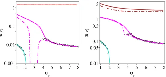
Figure 1. Left: Normalized real part of the KAW frequency ω{pkzcAq for βKe “ 1, τ} “ 1,

Θe“ 1, α “ 89˝, as a function of kdi, calculated using GF4 (black diamond symbols) and GF6L

(blue diamond symbols) models (respectively without and with Landau damping) and with the gyrokinetic dispersion relations GKNL (green solid line) and GK (red solid line). Middle: Damping rate from the GK theory (red solid line) and from the GF6L model (blue diamond symbols). Right: Normalized growth rate of the firehose instability as a function of kdi, for

βKe “ 0.5, τ} “ 10´3, Θe “ 0.16, α “ 89˝, as predicted by GF4 and GF6L models, together

with GKNL and GK dispersion relations, using the same graphic conventions.

essentially decoupled. The influence of the ion closure relation on the KAW properties thus remains limited. Deviations from the gyrokinetic theory at small scales are mostly due to the fact that when reaching these scales ζe “

a me{mi

a

2Θe{βKe ω{p|kz|cAq

becomes non-negligible.

4.3. SW dispersion relation and field swelling instability

Figure 2 concerns a similar comparison in the case of the field swelling instability discussed in Appendix C, for βKe“ 1, τ}“ 1, α “ 89˝, Θe“ 2.2 (left). For both the cases

with and without Landau damping, the relatively good agreement found at large scale between the gyrofluid theories and the gyrokinetic ones deteriorates at smaller scales. The stabilization scale is however correctly captured. This discrepancy is associated with a value of ζi, which is not small enough (in this case, ζe remains reasonably small). We

show in Fig. 2 (right) with Θe “ 2.41, again with βKe “ 1 and α “ 89˝, that a much

better agreement can be found when ions are hotter (τ_}“ 50), which prescribes a small ζi. The case with cold ions (τ} “ 10´5), for which the ion dynamics is decoupled, is

displayed in Fig. 3, showing an even better agreement. The left panel displays the real part of the slow wave for Θe “ 1, obtained with the GKNL model (solid green line)

or the GF4 model (diamond symbols). The right panel shows the growth rate of the field-swelling instability for Θe“ 2.01 (keeping unchanged the other parameters).

5. Conclusion

We derived a 6-field Hamiltonian gyrofluid model, referred to as GF6, retaining the gyrocenter density, the parallel velocity and temperature fluctuations for each species, under the sole assumption that all the other gyrocenter moments are calculated from the quasi-static linear kinetic theory. Such an assumption on the closure turns out to yield exact expressions for all the terms of the model, without, in particular, requiring approximated expressions for the terms involving gyroaverage operators. Nonlinear terms involving more than one gyroaverage operator, in particular, appear in the form of a single canonical bracket, which naturally lets the model fit in the class of Hamiltonian models with a Lie-Poisson structure. The model accounts for equilibrium temperature

Figure 2. Normalized growth rate of the field swelling instability versus kdi for α “ 89˝

and βKe “ 1, Left: Predictions of GF4 and GF6L, compared with those of GKNL and GK

respectively, for τ}“ 1 and Θe“ 2.2. Right: Prediction of GF4 compared with that of GKNL,

for τ}“ 50 and Θe“ 2.41 . Same graphic conventions as in Fig. 1 are used.

Figure 3. Left: Normalized slow-wave frequency versus kdiin regimes where the ions are cold

(τ} “ 10´5), with βKe “ 1 and α “ 89˝, as predicted by the GF4 model and the GKNL

dispersion relation. Right: normalized growth rate of the swelling instability for τ}“ 10´5 and

Θe“ 2.01. Same conventions as in Fig. 1 are used.

anisotropy and also retains both ion and electron FLR corrections, electron inertia and parallel magnetic fluctuations. In a variant of the model (GF6L) parallel Landau damping is retained through a Landau-fluid modelization of the gyrocenter parallel heat fluxes. A second variant of the model (GF4) is obtained by prescribing parallel isothermality, which still falls in the frame of the quasi-static closure and allows for a Hamiltonian formulation. The comparison of the dispersion relations of KAWs and SWs predicted from GF6L or GF4, with those derived from the parent gyrokinetic theory where the plasma response function is replaced by a Pad´e approximant, provides an estimate of the maximal transverse wavenumber beyond which the phase velocity of the corresponding

wave is too large compared with the electron (in the former case) or ion (in the latter case) parallel thermal velocity for consistency with a closure condition based on a quasi-static assumption. It turns out that the agreement extends to transverse scales significantly smaller than the ion Larmor radius in the case of KAWs, mostly because, at least at the linear level, SWs and KAWs are essentially decoupled, making the influence of the ion closure relation on the KAW properties relatively limited. This situation contrasts with the case of the SWs for which the dispersion relation is accurately reproduced only at scales larger than a significant fraction of the ion Larmor radius. Under these conditions, the model reproduces the instabilities induced by temperature anisotropy, such as firehose or field-swelling instabilities. It should nevertheless be noted that, as it assumes small perturbations of an equilibrium state, the model does not permit evolution of the mean temperatures, an effect usually considered as contributing efficiently to the saturation of these instabilities. The subcritical nonlinear regime is however expected to be accurately described. The model will in particular be most useful for studying the coupling of KAWs with SWs which can generate large-scale parametric decay instabilities at small βe, a regime especially relevant in the regions of the solar wind relatively close

to the Sun explored by space missions such as Parker Solar Probe or Solar Orbiter. In general, to the best of our knowledge, our gyrofluid model is the only one, at the present moment, possessing the following features, which could make it a valuable tool for local investigations of basic plasma phenomena of interest for space plasmas: it accounts for equilibrium temperature anisotropies as well as parallel magnetic perturbations; it reproduces, in a rather wide range of values of parameters, compatible with the quasi-static closure, quantitative features of known kinetic linear dispersion relations; the model equations, and in particular the terms involving FLR corrections, are calculated exactly, unlike other gyrofluid models which adopt truncations or approximations of such terms; it possesses a Hamiltonian structure.

Appendix A. Derivation of closure relations from the gyrokinetic

linear theory

We consider the linearization of the gyrokinetic system (2.1)-(2.4) about the equilib-rium stateg_rs“ 0 (or, equivalently, rfs“ 0), with rφ “ rAk“ rBk “ 0. The resulting linear

system can be written in the form B Bt ˜ r fs` qs T0ks v<sub>}</sub> c FeqsJ0sArk ¸ ` v} B Bz ˜ r fs` qs T0ks Feq<sub>s</sub> ˜ J0sφ ` 2r µsB0 qs J1s r B_k B0 ¸¸ “ 0, (A 1) ÿ s qs ż dWsJ0sfrs“ ÿ s q2 s T0Ks ż dWsFeq_s`1 ´ J0s2 ˘ r φ ´ÿ s qs ż dWs2 µsB0 T0Ks Feq<sub>s</sub>J0sJ1s r B<sub>k</sub> B0 , (A 2) ÿ s qs ż dWsv}J0sfrs “ ´ c 4π∇ 2 KArk` ÿ s q2_s ms ż dWsFeq_s ˜ 1 ´ 1 Θs v2_} v2 thks ¸ p1 ´ J0s2q r Ak c , (A 3) ÿ s βKs n0 ż dWs2 µsB0 T0Ks J1sfrs“ ´ ÿ s βKs n0 qs T0Ks ż dWs2 µsB0 T0Ks Feq_sJ0sJ1sφr ´ ˜ 2 `ÿ s βKs n0 ż dWsFeq_s ˆ 2µsB0 T0Ks J1s ˙2¸ r Bk B0 , (A 4)

where we adopted the same notation with the tilde symbol, that we used in Eqs. (2.1)-(2.4), to indicate the dynamical variables rfsof the linearized system and the field

perturbations rφ, rAk and rBk.

We introduce the following Fourier series representation: r fspx, v}, µs, tq “ ÿ kPD r fskpv}, µsqeipk¨x´ωtq, φpx, tq “r ÿ kPD r φkeipk¨x´ωtq, (A 5) r Akpx, tq “ ÿ kPD r Akkeipk¨x´ωtq, Br_kpx, tq “ ÿ kPD r Bkkeipk¨x´ωtq, (A 6)

with ω P C indicating the complex frequency.

For any given k PD, from Eq. (A 1) we obtain the relation r fsk “ r ζs pv}{vthksq ´ rζs v_} c qs T0ks Feq_sJ0pasq rAkk ´ 1 pv}{vthksq ´ rζs v} vthks Feq_s ˜ qs T0ks J0pasq rφk` 2µsB0 T0ks J1pasq as r Bkk B0 ¸ , (A 7) where rζs“ ω{pkzvthksq.

We consider now the quasi-static limit | rζs| ! 1. In this limit, the relation (A 7) reduces

to r fsk “ ´Feqs ˜ qs T0ks J0pasq rφk` 2µsB0 T0ks J1pasq as r Bkk B0 ¸ . (A 8)

In the following, we make use of the relation (A 8), derived from the linear theory, in order to determine the closure relations to insert in the hierarchy of nonlinear gyrofluid equations. For this purpose, we adopt the Hermite-Laguerre expansion of Eq. (3.18) for the perturbation of the distribution function in the linearized system and we write

r fspx, v}, µs, tq “ Feq_spv}, µsq `8 ÿ m,n“0 1 ? m!Hm ˜ v} vthks ¸ Ln ˆ µsB0 T0Ks ˙ fmnspx, tq (A 9) with fmnspx, tq “ ÿ kPD fmnske ipk¨x´ωtq _{(A 10)}

in Fourier representation. From Eqs. (A 9), (A 10), using the orthogonality relations for Hermite and Laguerre polynomials, one obtains

fmnsk “ 1 n0 ? m! ż dWsfrskHm ˜ v_} vthks ¸ Ln ˆ µsB0 T0Ks ˙ . (A 11)

Inserting the relation (A 8) into Eq. (A 11) and using the orthogonality relations for Hermite polynomials, one has

fmnsk “ ´δm0 ˜ G1n qs T0ks r φk` 2ΘsG2n r B_kk B0 ¸ , (A 12)

where the operators G1n and G2n are defined by

G1n “ 2πB0 ms ż dµsfeqspµsqLn ˆ µsB0 T0Ks ˙ J0pasq, (A 13) G2n “ 2πB0 ms ż dµsfeqspµsqLn ˆ µsB0 T0Ks ˙ µsB0 T0Ks J1pasq as , (A 14) with feqspµsq “ ms 2πT0Ks e´ µsB0 T0_{Ks. (A 15)}

Explicit expressions for the operators G1n and G2n can be found by computing the

integrals in Eqs. (A 13) and (A 14), which yields G1npbsq “ e´bs{2 n! ˆ bs 2 ˙n , n ě 0, (A 16) G20pbsq “ e´bs{2 2 , G2npbsq “ ´ e´bs{2 2 ˜ ˆ bs 2 ˙n´1 1 pn ´ 1q! ´ ˆ bs 2 ˙n 1 n! ¸ , n ě 1. (A 17) In order to obtain the expressions (A 16)-(A 17) use was made of the orthogonality of Laguerre polynomials as well as of the relations (Szeg¨o 1975)

J0pasq “ e´bs{2 `8 ÿ n“0 Ln ´ µsB0 T<sub>0Ks</sub> ¯ n! ˆ bs 2 ˙n , (A 18) 2J1pasq as “ e´bs{2 `8 ÿ n“0 Lp1qn ´ µsB0 T_0Ks ¯ pn ` 1q! ˆ bs 2 ˙n , (A 19)

where Lp1qn is a generalized Laguerre polynomial. Making use of the Fourier

representa-tions (A 10) , (A 5) and (A 6) for for fmns, rφ and rBk, respectively, one can deduce from

Eq. (A 12) the relation

fmnspx, tq “ ´δm0 ˜ G1ns qs T0ks r φ ` 2ΘsG2ns r Bk B0 ¸ , (A 20) or, equivalently, fmnspx, tq “ ´δm0Θs ˆ sgnpqsqG1ns φ τ<sub>Ks</sub> ` 2G2nsBk ˙ , (A 21)

where we also made use of the normalization (3.11) for φ and Bk. The operators

G1ns and G2ns are defined, consistently with the definition of G10s and G20s

given in Sec. 3, by G1nsf px, tq “ ř_kPDG1npbsqfkptq exppik ¨ xq and G2nsf px, tq “

ř

kPDG2npbsqfkptq exppik ¨ xq, for a function f and n ě 0 (in the specific case of the

linear dispersion relation, the dependence on t is provided by the factor e´iωt_{, but when}

the relations (A 21) are used as closures for the nonlinear models, the dependence on t is of course left arbitrary).

The relations (A 21) descending from the quasi-static assumption, are adopted as closure relations in GF6 and GF6L for all the moments involved in the model, except for Ns, Ms, Tks, which are derived by solving the evolution equations (3.3)-(3.5). The parallel

heat flux fluctuations Qks, on the other hand, are determined, as already mentioned,

again by a quasi-static closure for GF6 (Eq. (3.23) which follows from Eq. (A 21) for m “ 3, n “ 0) or by the Landau closure (3.35) for GF6L. The closure (3.36) adopted for GF4, is again a quasi-static closure following from Eq. (A 21) when m “ 2 and n “ 0.

Appendix B. Derivation of the model equations

The gyrofluid system (3.3)-(3.8) descends from the parent gyrokinetic system (2.1)-(2.4) upon applying to the perturbations of the distribution functions the expansion (3.18). In order to obtain a closed system with a finite number of equations, such expansion is constrained in the following way. The moments f00s, f10s and f20s (or,

equivalently, by virtue of Eqs. (3.20)-(3.21), the gyrofluid densities, parallel velocities and temperatures Ns, Us and Tks), for each species s, get determined by evolution

equations obtained by making the product of all the terms of the gyrokinetic equation (2.1) with the zero, first and second order Hermite polynomial in the variable v_}{vthks

and integrating over the velocity volume element dWs. For GF6L, the parallel heat flux

Q_ks gets determined by the relation (3.35). All the other moments, on the other hand, are assumed to be given by the relations (A 20), or, in normalized form, by Eq. (A 21), obtained from the linear theory in the quasi-static limit. With this prescription, the expansion (3.18) becomes r fspx, v}, µs, tq “ Feq_spv}, µsq ˜ r Ns n0 px, tq ` v} vthks r Us vthks px, tq `1 2 ˜ v2 } v_th2 ks ´ 1 ¸ r Tks T0ks px, tq ` 1 6 ˜ v3 } v<sub>th</sub>3 ks ´ 3 v} vthks ¸ r Qks n0T0ksvthks px, tq ´ `8 ÿ n“1 Ln ˆ µsB0 T0Ks ˙˜ G1ns qs T0ks r φpx, tq ` 2ΘsG2ns r Bk B0 px, tq ¸¸ , (B 1)

where we made use of the fact that H0pv}{vthksq “ 1, H1pv}{vthksq “ v}{vthks, H2pv}{vthksq “ v 2 }{v 2 thks´ 1 and H3pv}{vthksq “ v 3 }{v 3 thks´ 3v}{vthks.

Inserting the expansion (B 1) into Eqs. (2.5) and (2.1), and integrating over dWsone

obtains B Bt r Ns n0 ` c B0 ˜« G10sφ,r r Ns n0 ff ´ `8 ÿ n“1 « G1nsφ,r qs T0ks G1nsφ ` 2Θr <sub>s</sub>G<sub>2ns</sub> r Bk B0 ff ´ `8 ÿ n“1 « 2T0Ks qs G2ns r Bk B0 , qs T0ks G1nsφ ` 2Θr <sub>s</sub>G<sub>2ns</sub> r Bk B0 ff `T0Ks qs « 2G20s r Bk B0 ,Nrs n0 ff (B 2) ´ « G1nsAr_k, r Us c ff¸ `B rUs Bz “ 0,

where we made use of the definitions (A 13) and (A 14) and of the orthogonality of Hermite polynomials. We remark, at this point, that the sum of the last term in the first line of Eq. (B 2) with the first term on the second line of Eq. (B 2) yields zero, because of the antisymmetry of the canonical bracket r , s. We thus conclude that the quasi-static closure (A 20) has the remarkable property of annihilating, in the continuity equation, all the contributions associated with the moments f0ns, for n ě 1. By virtue of this

cancellation, from Eq. (B 2) we obtain

B Bt r Ns n0 ` c B0 « G10sφ `r T0Ks qs 2G20s r Bk B0 ,Nrs n0 ff ´ 1 B0 ” G10sAr_k, rUs ı `B rUs Bz “ 0. (B 3)

Applying to Eq. (B 3) the normalization (3.9)-(3.12), one obtains Eq. (3.3).

In order to derive Eq. (3.4) we point out first that, with the help of the identities

J0pasq “ e´bs{2 `8 ÿ n“0 Ln ´ µsB0 T<sub>0Ks</sub> ¯ n! ˆ bs 2 ˙n , (B 4) 2J1pasq as “ e´bs{2 `8 ÿ n“0 Lp1qn ´ µsB0 T_0Ks ¯ pn ` 1q! ˆ bs 2 ˙n , (B 5) ż`8 0 dx e´x_L npxqLmpxq “ δmn, (B 6) Lp1q mpxq “ ´ d dxLm`1pxq “ ´ m ` 1 x Lm`1pxq ` m ` 1 x Lmpxq, (B 7)

we obtain the relation (see also Brizard (1992)) c B0 ż dWsFeq_s « J0sφ,r qs T0ks v2_} vthksc J0sAr_k ff (B 8) “ n0 vthks B0 ÿ k,k1_PD ż dˆ µsB0 T0Ks ˙ e´µsB0{T_0Ks ˆ « qs T0ks J0 ˆ k_K ωcs c 2µsB0 ms ˙ r φ, J0 ˜ k_K1 ωcs c 2µsB0 ms ¸ qs T0ks r A_k ff eipk`k1q¨x <sub>(B 9)</sub> “ n0 vthks B0 ÿ k,k1<sub>PD</sub> `8 ÿ m,n“0 ż dˆ µsB0 T0Ks ˙ e´µsB0{T_0Ks ˆ » – qs T0ks e´bs{2 Lm ´ µsB0 T_0Ks ¯ m! ˆ bs 2 ˙m r φ, e´b1s{2 Ln ´ µsB0 T_0Ks ¯ n! ˜ b1_s 2 ¸n r A_k fi fleipk`k 1<sub>q¨x</sub> “ n0 vthks B0 `8 ÿ n“0 « qs T0ks G1nsφ, Gr 1nsAr_k ff , (B 10)

and, by an analogous procedure, the relation

c B0 ż dWsFeqs « 2µsB0 qs J1s r Bk B0 , qs T0ks v2 } vthksc J0sAr_k ff “ n0Θs vthks B0 `8 ÿ n“0 « 2G2ns r Bk B0 , G1nsAr_k ff . (B 11)

Upon multiplying Eq. (2.1) by p1{n0qv}{vthks and integrating over dWs one obtains,

adopting the expansion (B 1) as well as the relations (A 13), (A 14), (B 10) and (B 11), the following equation

B Bt ˜ r Us vthks ` qs T0ks vthks c G10sArk ¸ ` c B0 « G10sφ `r T0Ks qs 2G20s r Bk B0 , Urs vthks ff ` vthks B0 `8 ÿ n“0 « qs T0ks G1nsφ ` 2Θr sG2ns r Bk B0 , G1nsAr_k ff ´ vthks B0 « G10sAr_k, r Ns n0 ` r Tks T0ks ff `vthks B0 `8 ÿ n“1 « G1nsAr<sub>k</sub>, qs T0ks G1nsφ ` 2Θr sG2ns r Bk B0 ff (B 12) ` vthks B Bz ˜ r Ns n0 ` qs T0ks G10sφ ` 2Θr sG20s r B<sub>k</sub> B0 ` Trks T0ks ¸ “ 0.

Also in this case, the quasi-static closure leads to a remarkable cancellation. Indeed, among the nonlinear terms involving only electromagnetic quantities (i.e. rφ, rAkand rBk)

result, Eq. (B 12) reduces to B Bt ˜ r Us vthks ` qs T0ks vthks c G10sArk ¸ ` c B0 « G10sφ `r T0Ks qs 2G20s r Bk B0 , Urs vthks ff `vthks B0 « qs T0ks G10sφ ` 2Θr sG20s r B<sub>k</sub> B0 , G10sAr<sub>k</sub> ff ´vthks B0 « G10sAr<sub>k</sub>, r Ns n0 ` Trks T0ks ff (B 13) ` vthks B Bz ˜ r Ns n0 ` qs T0ks G10sφ ` 2Θr sG20s r B<sub>k</sub> B0 ` Trks T0ks ¸ “ 0.

Equation (3.4) is then obtained from Eq. (B 13) after applying the normalization (3.9)-(3.12).

Equation (3.5) is obtained upon multiplying Eq. (2.1) by p1{n0qpv_}2{vth2ks´ 1q and

integrating over dWs. Making use of the expansion (B 1) and of the orthogonality of

Hermite polynomials one obtains B Bt r Tks T0ks ` c B0 ˜« G10sφ,r r Tks T0ks ff `T0Ks qs « 2G20s r Bk B0 , Trks T0ks ff ´2 « G10sAr_k, r Us c ff ´ « G10sAr_k, r Qks n0T0ksc ff¸ ` vthks B Bz ˜ 2 Urs vthks ` Qrks n0T0ksvthks ¸ “ 0. (B 14)

Adopting the normalization (3.9)-(3.12), Eq. (3.5) follows from Eq. (B 14).

Equations (3.6), (3.7) and (3.8) follow from Eq. (2.2), (2.3) and (2.4), respectively, upon inserting the expansion (B 1), evaluating the integrals and applying the normalization (3.9)-(3.12). With regard to the evaluation of the integrals and the derivation of the equations in the form (3.6), (3.7) and (3.8), we remark that, in addition to Eqs. (A 13)-(A 14), the following relations are of use:

1 n0 ż dWsFeq_sJ02pasq “ Γ0pbsq “ `8 ÿ n“0 G21npbsq, (B 15) 1 n0 ż dWsFeq<sub>s</sub> 2µsB0 T0Ks J0pasq J1pasq as “ Γ0pbsq ´ Γ1pbsq “ G210pbsq ` 2 `8 ÿ n“1 G1npbsqG2npbsq, (B 16) 1 n0 ż dWsFeq<sub>s</sub> ˆ 2µsB0 T0Ks J1pasq as ˙2 “ 2pΓ0pbsq ´ Γ1pbsqq “ G210pbsq ` 4 `8 ÿ n“1 G2_2npbsq. (B 17)

Appendix C. Field-swelling instabilities

C.1. Dispersion relation at the MHD scales

In this Appendix, we first provide a simple derivation of the dispersion relation for fast and slow modes at MHD scales in the presence of temperature anisotropy, starting from the kinetic-MHD equations (see Eqs. (37), (38b), (44 a,b,c) (46)-(48) from Kulsrud (1983), or equivalently Eqs. (1)-(8) from Snyder et al. (1997)).

The transverse velocity can be decomposed into compressible and solenoidal parts by writing

u_K“ ´∇Kχc` ∇Kˆ pχspzq. (C 1)

One immediately gets (see e.g. Eqs. (48),(52) and (56) of Passot & Sulem (2006) where FLR corrections are neglected)

´BtBxxχc` Bxx ´<sub>p</sub> K ρ0 ` c2A B_} B0 ˘ ``c2A` p0K´ p0} ρ0 ˘ Bzz B_} B0 “ 0, (C 2) Bt B_} B0 ´ Bxxχc“ 0, (C 3)

where pKand p} denote the total (ion plus electron) perpendicular and parallel pressure

fluctuations, with the subscript 0 referring to the equilibrium values. Furthermore, ρ0

denotes the equilibrium plasma density.

In Eq. (C 2), the perpendicular pressure fluctuations are given by the drift-kinetic theory, as found e.g. in Eq. (27) of Snyder et al. (1997), in the form

pKr ρ0 “ T0Kr mi ˆ 2p1 ´ ΘrRpζrqq B} B0 ´ Rpζrq qrψ T_}r ˙ , (C 4) together with nr n0 “ p1 ´ ΘrRpζrqq B_} B0 ´ Rpζrq qrψ T}r , (C 5)

where qr “ e for ions and ´e for electrons, respectively. The potential ψ is defined in

terms of the parallel electric field by Ez“ ´Bzψ. These expressions for the perpendicular

pressure and density perturbations identify with the large-scale limit of formulas given in Appendix B of Passot & Sulem (2007). Quasineutrality requires the equality of the electron (ne) and ion (ni) number-density fluctuations, which prescribes

eψ T0ke “ τ} ΘeRpζeq ´ ΘiRpζiq τ_}Rpζeq ` Rpζiq B_} B0 . (C 6)

Plugging the expressions for the pressures in Eqs. (C 2)-(C 3) thus leads to ω2 k2_c2 A “1 ´k 2 z k2 β_}e 2 p1 ´ Θe` τ}p1 ´ Θiqq `k 2 K k2 βKe 2 ” 2p1 ´ ΘeRpζeqq ` τKip2 ´ ΘeRpζeq ´ ΘiRpζiqq ` τ}p1 ` τKiqRpζeq ´<sub>ΘeRpζeq ´ ΘiRpζiq</sub> τ<sub>}</sub>Rpζeq ` Rpζiq ¯ı . (C 7) We note that ζ_i2“ ω 2 2τ_}ω2 s with ωs“ kzcs} where cs} “ d T0ke mi

is the sound speed based on the parallel electron temperature.

C.2. Link with the fluid theory

In order to make a link with fluid theory as performed in Basu & Coppi (1984), we note that keeping all the terms in the ion density and parallel velocity equations (in particular the time derivatives), is equivalent to expanding Rpζiq for ζi large, i.e. in the

adiabatic limit where Rpζiq « ´1{p2ζi2q. It thus follows that the ions cannot be hot, at