Extrasolar planets and brown dwarfs around AF-type stars

HAL Id: hal-01994794

https://hal.sorbonne-universite.fr/hal-01994794

Submitted on 25 Jan 2019

HAL is a multi-disciplinary open access

archive for the deposit and dissemination of

sci-entific research documents, whether they are

pub-lished or not. The documents may come from

teaching and research institutions in France or

abroad, or from public or private research centers.

L’archive ouverte pluridisciplinaire HAL, est

destinée au dépôt et à la diffusion de documents

scientifiques de niveau recherche, publiés ou non,

émanant des établissements d’enseignement et de

recherche français ou étrangers, des laboratoires

publics ou privés.

stars

S. Borgniet, A.-M. Lagrange, N. Meunier, F. Galland, L. Arnold, N.

Astudillo-Defru, J.-L. Beuzit, I. Boisse, X. Bonfils, F. Bouchy, et al.

To cite this version:

S. Borgniet, A.-M. Lagrange, N. Meunier, F. Galland, L. Arnold, et al.. Extrasolar planets and

brown dwarfs around AF-type stars: X. The SOPHIE sample: combining the SOPHIE and HARPS

surveys to compute the close giant planet mass-period distribution around AF-type stars. Astronomy

and Astrophysics - A&A, EDP Sciences, 2019, 621, pp.A87. �10.1051/0004-6361/201833431�.

�hal-01994794�

Astronomy

_&

Astrophysics

© ESO 2019

Extrasolar planets and brown dwarfs around AF-type stars

X. The SOPHIE sample: combining the SOPHIE and HARPS surveys to compute

the close giant planet mass-period distribution around AF-type stars

?

??

S. Borgniet

_{, A.-M. Lagrange}

_{, N. Meunier}

_{, F. Galland}

_{, L. Arnold}

_{, N. Astudillo-Defru}

_{, J.-L. Beuzit}

_,

I. Boisse

_{, X. Bonfils}

_{, F. Bouchy}

_{, K. Debondt}

_{, M. Deleuil}

_{, X. Delfosse}

_{, M. Desort}

_{, R. F. Díaz}

_,

A. Eggenberger

_{, D. Ehrenreich}

_{, T. Forveille}

_{, G. Hébrard}

_{, B. Loeillet}

_{, C. Lovis}

_{, G. Montagnier}

_,

C. Moutou

_{, F. Pepe}

_{, C. Perrier}

_{, F. Pont}

_{, D. Queloz}

_{, A. Santerne}

_{, N. C. Santos}

_{, D. Ségransan}

_,

R. da Silva

_{, J. P. Sivan}

_{, S. Udry}

_{, and A. Vidal-Madjar}

e-mail: simon.borgniet@obspm.fr

2 _{Observatoire de Haute-Provence, Institut Pythéas UMS 3470, CNRS, Aix-Marseille Université, 04870 St-Michel-l’Observatoire,}

France

3 _{Departamento de Astronomía, Universidad de Concepción, Casilla 160-C, Concepción, Chile}

4 _{LAM (Laboratoire d’Astrophysique de Marseille) UMR 7326, CNRS, Aix Marseille Université, 13388 Marseille, France} 5 _{Observatoire Astronomique de l’Université de Genève, 51 Chemin des Maillettes, 1290 Versoix, Switzerland}

6 _{Institut d’Astrophysique de Paris, UMR 7095 CNRS, Université Pierre & Marie Curie, 98 bis Boulevard Arago, 75014 Paris,}

France

7 _{Canada-France-Hawaii Telescope Corporation, 65-1238 Mamalahoa Hwy, Kamuela, HI 96743, USA}

8 _{Cavendish Laboratory, J J Thomson Avenue, Cambridge CB3 0HE, UK}

9 _{Instituto de Astrofísica e Ciências do Espaço, Universidade do Porto, CAUP, Rua das Estrelas, 4150-762 Porto, Portugal}

10_{Departamento de Física e Astronomia, Faculdade de Ciências, Universidade do Porto, Rua do Campo Alegre, 4169-007 Porto,}

Portugal

11_{ASI – Space Science Data Center (SSDC), Via del Politecnico snc, 00133 Rome, Italy}

12_{INAF – Osservatorio Astronomico di Roma, Via Frascati 33, 00078 Monte Porzio Catone, Rome, Italy}

Received 15 May 2018 / Accepted 30 August 2018

ABSTRACT

Context. The impact of stellar mass on the properties of giant planets is still not fully understood. Main-sequence (MS) stars more

massive than the Sun remain relatively unexplored in radial velocity (RV) surveys, due to their characteristics which hinder classical RV measurements.

Aims. Our aim is to characterize the close (up to ∼2 au) giant planet (GP) and brown dwarf (BD) population around AF MS stars and

compare this population to stars with different masses.

Methods. We used the SOPHIE spectrograph located on the 1.93 m telescope at Observatoire de Haute-Provence to observe 125

north-ern, MS AF dwarfs. We used our dedicated SAFIR software to compute the RV and other spectroscopic observables. We characterized the detected substellar companions and computed the GP and BD occurrence rates combining the present SOPHIE survey and a similar HARPS survey.

Results. We present new data on two known planetary systems around the F5-6V dwarfs HD 16232 and HD 113337. For the latter,

we report an additional RV variation that might be induced by a second GP on a wider orbit. We also report the detection of 15 binaries or massive substellar companions with high-amplitude RV variations or long-term RV trends. Based on 225 targets observed with SOPHIE and/or HARPS, we constrain the BD frequency within 2–3 au around AF stars to be below 4% (1σ). For Jupiter-mass GPs within 2–3 au (periods ≤103 _{days), we find the occurrence rate to be 3.7}+3

−1% around AF stars with masses <1.5 M, and to be

≤6% (1σ) around AF stars with masses >1.5 M. For periods shorter than 10 days, we find the GP occurrence rate to be below 3 and

4.5% (1σ), respectively. Our results are compatible with the GP frequency reported around FGK dwarfs and are compatible with a possible increase in GP orbital periods with stellar mass as predicted by formation models.

Key words. techniques: radial velocities – stars: early-type – planetary systems – stars: variables: general

?_{Based in part on observations made at Observatoire de Haute Provence (CNRS), France.}

??_{RV time series of the full sample are only available at the CDS via anonymous ftp tocdsarc.u-strasbg.fr(130.79.128.5) or via}

http://cdsarc.u-strasbg.fr/viz-bin/qcat?J/A+A/621/A87

A87, page 1 of30

Open Access article,published by EDP Sciences, under the terms of the Creative Commons Attribution License (http://creativecommons.org/licenses/by/4.0), which permits unrestricted use, distribution, and reproduction in any medium, provided the original work is properly cited.

1. Introduction

More than three thousand exoplanets and brown dwarfs (BDs) have now been confirmed1_{, while thousands of other Kepler}

can-didates await confirmation. Most of these substellar companions are close (≤5–10 au) to their host star and have been detected via radial velocity (RV) and transit surveys (see e.g. Borucki et al. 2010;Howard et al. 2011;Fressin et al. 2013;Mayor et al. 2014). Giant gaseous planets are at the core of the planetary sys-tems as they carry most of their mass. These close giant planets (GPs) have revealed an unexpected diversity of orbital (period, eccentricity, inclination) and physical (mass, composition) prop-erties. This variety emphasizes the complexity of the different processes and interactions that shape the GP population in terms of formation, migration, dynamical interactions, or influence of the primary host star.

While our understanding of the GP formation and evolu-tion mechanisms has dramatically improved over the past twenty years, the influence of stellar properties on GP distribution remains a key topic. For example, it has been clearly estab-lished that the GP frequency increases with stellar metallicity for solar-like, main-sequence (MS) FGK dwarfs (Santos et al. 2004;

Fischer & Valenti 2005).

However, the impact of the stellar host mass on its compan-ion’s properties is still not fully understood. The core-accretion formation process, which is believed to be at the origin of most of the RV and transit planets, predicts an increase in GP fre-quency with stellar mass (up to 3–3.5 M,Kennedy & Kenyon

2008). This was confirmed by comparing the GP occurrence rates derived from RV surveys of low-mass M dwarfs (see e.g.

Bonfils et al. 2013) and of solar-mass FGK dwarfs (see e.g.

Cumming et al. 2008). Subgiant and giant stars seem to confirm this trend for higher stellar masses, as higher GP occurrence rates than those found around solar-mass dwarfs have been reported for these evolved stars (see e.g.Johnson et al. 2010;Reffert et al. 2015). However, the actual mass and origin of these evolved stars is subject to an ongoing controversy, as several studies argue that these giants do not significantly differ from solar-type stars in terms of mass, and are consequently their descendants (instead of being the descendants of AF MS stars; see the list of references inBorgniet et al. 2017).

AF stars with well-established masses above 1 M on the

main sequence are generally rejected from RV surveys because their specific characteristics (fewer spectral lines and faster rota-tion) hinder classical RV measurements. A recent survey has targeted chemically peculiar Ap stars, which exhibit lower rota-tional velocities and more narrow spectral lines than typical AF MS dwarfs (Hartmann & Hatzes 2015).

Twelve years ago our group developed a tool, Software for the Analysis of the Fourier Interspectrum Radial velocities (SAFIR,Galland et al. 2005b), specifically dedicated to deriv-ing RV measurements of AF MS stars as precisely as possible. For one target, SAFIRcross-correlates each observed spectrum with a reference spectrum built from all the acquired spectra instead of a binary mask, allowing one to reach a better RV pre-cision (closer to the photon noise limit defined byBouchy et al. 2001). Even if this RV precision remains intrinsically degraded compared to cooler and/or slower rotating stars, we developed SAFIR(and other specific tools) to demonstrate that it is indeed possible to search for close (.3 au) massive (≥1 MJup) GP and

BD companions around AF MS stars (Galland et al. 2005a,2006;

Lagrange et al. 2009;Meunier et al. 2012).

1 _{http://exoplanet.eu,Schneider et al.(2011).}

From 2005 to 2016, we carried out a survey targeting GPs and BDs orbiting within ∼3 au around southern AF MS dwarfs with the High-Accuracy Radial velocity Planet Searcher (HARPS, see

Pepe et al. 2002) spectrograph on the 3.6 m ESO telescope at La Silla Observatory in Chile. During this survey, we detected three new GPs around two F5-6V stars (Desort et al. 2008), showed that GPs more massive than Jupiter and BDs are often detectable at periods of up to a thousand days around MS AF dwarfs more massive than the Sun (Lagrange et al. 2009), and derived the first constraints on the occurrence rates of such companions (Borgniet et al. 2017, hereafter PaperIX). Meanwhile, we carried out a survey of northern AF MS stars with the SOPHIEechelle fibre-fed spectrograph (Bouchy & Sophie Team 2006), which is the successor of the ELODIEspectrograph (Baranne et al. 1996) on the 1.93 m telescope at Observatoire de Haute-Provence in France. Most of the observations were made in the course of the SP4 programme within the SOPHIE consortium (Bouchy et al. 2009). The first results of our SOPHIEsurvey, regarding the complex RV variations of HD 185395 and the detection of a ∼3 MJupGP orbiting with a ∼320-day period around HD 113337,

were presented inDesort et al.(2009) andBorgniet et al.(2014), respectively.

This paper first presents our SOPHIE survey and its results, and then presents a statistical analysis combining our

SOPHIE and HARPStargets from Paper IX to make a single,

global study. The SOPHIE-HARPScombination is possible here because (i) the HARPS and SOPHIE instruments work on the same principles, (ii) they have a similar instrumental RV pre-cision (less than 1 m s−1 _{for HARPS versus a few m s}−1 _for

SOPHIE), (iii) our surveys have the same overall characteristics, and (iv) we use exactly the same reduction and analysis that we used for our HARPSsample in PaperIX. In Sect.2, we describe our SOPHIEsample and observations and give a brief outline of our computational tool, our observables, and our RV variability diagnosis. Section3is dedicated to the detection and character-ization of giant planets and other long-term companions within our SOPHIEsurvey. In Sect.4we make a global analysis of the combined SOPHIE+ HARPSsample: (i) we characterize the RV intrinsic variability of our targets, (ii) we derive the search pleteness of our combined survey, and (iii) we combine the com-panion detections and the detection limits to compute the close companion (GP and BD) occurrence rates and estimate their (mass, period) distribution around AF MS stars. We conclude in Sect.5.

2. Description of the SOPHIEsurvey

2.1. Sample

Our SOPHIEsample is made up of 125 AF MS dwarf stars with spectral types in the range A0V to F9V. We detail the physical properties of our sample in AppendixA. We selected our tar-gets using the same selection process as for our HARPSsurvey (see details inLagrange et al. 2009, PaperIXand AppendixB). Briefly, our selection relies on the following criteria: (i) the spectral type; (ii) the distance to the Sun, and (iii) the exclu-sion of known SB2 binary, chemically peculiar stars, or con-firmed δ Scuti or γ Doradus pulsators. We ended up with 125 targets with B − V in the range −0.02 to 0.56, v sin i in the range 3 to 250 km s−1_{, and masses in the range 1 to}

2.5 M(Fig.1). We note that the exclusion of known pulsators

results in a visible dichotomy between our ∼A- and ∼F-type targets.

Fig. 1.Main physical properties of our sample. Left panel: HR diagram of our sample, in absolute V-magnitude vs B−V. Each black dot corresponds to one target. The Sun (red star) is displayed for comparison. Middle panel: v sin i vs B − V distribution. Right panel: mass histogram of our sample (in M).

Fig. 2.Observation summary. Left panel: histogram of the spectrum number per target. Middle panel: histogram of the separate observation epoch

number per target. Right panel: histogram of the time baselines. 2.2. Observations

We observed our 125 SOPHIEtargets mainly between Novem-ber 2006 and April 2014. We made some additional observa-tions in 2015–2016 to complete our survey for the targets with the less data and to further monitor the most interesting tar-gets. We acquired the SOPHIEspectra in high-resolution mode (R ∼ 75000), in the 3872–6943 Å wavelength range. As was done with our HARPStargets, we adapted the exposure times depend-ing on the observdepend-ing conditions and on the target magnitude in order to get a high signal-to-noise ratio (S/N), of at least 100 at λ =550 nm. We made most of the exposures in the simultaneous-Thorium mode, for which the SOPHIEA fibre is centred on the target while the B fibre is fed by a Thorium lamp. This allowed us to follow and correct for a potential instrumental RV drift induced by local temperature or pressure variations, if needed. For very bright targets (very small exposure times), we acquired the spectra in the SOPHIEstandard spectroscopy mode (which is appropriate for very bright targets): the A fibre is centred on the target while the B fibre is not illuminated. Our observing strategy and analysis are fully detailed in PaperIX. Briefly, we acquired at least two consecutive spectra at each epoch/visit during sev-eral consecutive nights to estimate the short-term stellar jitter of our ∼F-type targets, whereas we acquired multiple consecutive spectra per epoch for our ∼A-type targets, to mitigate the effect of pulsations.

The median time baseline of our SOPHIEsurvey is 1448 days or ∼4 yr (the mean time baseline being 1640 days or 4.5 yr), with a median spectrum number per target of 23 (36 on average) acquired during a median number of 11 visits (17 on average, Fig.2).

2.3. Observables

As was done for our HARPS sample, we computed the RV and, whenever possible, the line profiles and the chromospheric emission in the calcium lines of our targets with our software SAFIR(Chelli 2000;Galland et al. 2005b). The main principles of SAFIRare fully detailed in Paper IX. Our main observables are the RV, the spectrum cross-correlation function (CCF) and its full width at half maximum (FWHM), the bissector velocity span (hereafter BIS;Queloz et al. 2001) and the logR0

HK. Our main

(but not the only) diagnosis for classifying the RV variability of our targets and distinguishing between its possible sources is the (RV, BIS) diagram; see PaperIX for a fully detailed descrip-tion of our various observables and of our variability criteria and diagnosis. Very briefly, we classify our targets as RV vari-able if the total RV amplitude and the RV standard deviation are respectively at least six and two times larger than the mean RV uncertainty. A RV–BIS anti-correlation is most likely the indication of stellar magnetic activity, a RV–BIS vertical dia-gram indicates pulsations and a flat RV–BIS diadia-gram points toward companionship; CCF distortions and/or RV–FWHM cor-relation might indicate the presence of a SB2 or SB1 binary. More detailed results on our target observables can be found in AppendixA.

It should be noted that we quadratically add 5 m s−1_of

sys-tematic error to the SOPHIEuncertainties to take into account the SOPHIEinstrumental error (Díaz et al. 2012;Bouchy et al. 2013;

Borgniet et al. 2014). Such an error may be slightly excessive for the latest SOPHIEmeasurements (see below), but we pre-fer to be conservative and keep the same uncertainty for all our data.

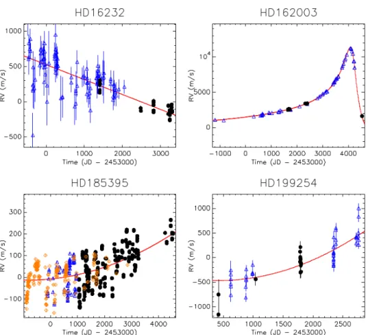
Table 1. Stellar properties of our targets with detected GPs. Parameter Unit HD 16232 HD 113337 Spectral type F6Va _F6Vb V 7.09c _6.03c B − V 0.5c _0.37c vsin i (km s−1_{) 30}c ₆c π (mas) 24.52 ± 0.68d 27.11 ± 0.29d [Fe/H] −0.03e 0.09e Teff (K) 6396 ± 95e 6669 ± 80e log g (dex) 4.44 ± 0.08f _{4.21 ± 0.08}f M? (M) 1.20 ± 0.09f 1.41 ± 0.09f Radius (R) 1.10 ± 0.05f 1.55 ± 0.07f Age (Gyr) 0.9 ± 0.8a _0.15+0.1 −0.05g

References. (a)_{Guenther et al.(2009).}(b)_{Boesgaard & Tripicco(1986).} (c)_{Taken from the CDS. The uncertainties on the v sin i are not provided.}

(d)_{van Leeuwen(2007).}(e)_{Casagrande et al.(2011). The catalog does not}

provide the uncertainties on the metallicity.(f )_{Allende Prieto & Lambert}

(1999).(g)_{Borgniet et al.(2014).}

2.4. SOPHIE+

In June 2011 (BJD 2455730), SOPHIEwas updated (and called

SOPHIE+) by implementing octagonal fibres at the fibre link

(Bouchy et al. 2013). Prior to this update, the SOPHIERV were known to exhibit a systematic bias induced by the insufficient scrambling of the old fibre link. This bias was called the “see-ing effect” as see“see-ing variations at the fibre entrance were caus“see-ing RV variations (Boisse et al. 2011). One way to correct for this bias is to measure the RV in the blue and red halves of each SOPHIEspectral order and compute their difference δRV, which

should be correlated to the original RV if affected by the seeing effect, as detailed inDíaz et al.(2012). We applied the same cor-rection in SAFIR, computing δRVfor all spectra acquired prior

to June 2011, and correcting the RV from the δRVcorrelation if

needed (i.e. if the Pearson’s correlation coefficient was above 0.5 in absolute value). This happened for 16 of our targets for which the δRVcorrelation was >0.5.

3. Detected companions in the SOPHIEsurvey

3.1. Giant planets

In this section we present two planetary systems with three GPs, either confirmed or probable candidates. The host stars’ fundamental properties are detailed in Table 1, and the orbital parameters of the detected and/or candidate GPs in Table2. The RV and line profile data of these systems are shown in detail in AppendixD.

3.1.1. HD 113337 system

Summary of first planet detection. We reported the detec-tion of a giant planet orbiting around HD 113337 and charac-terized it inBorgniet et al.(2014, hereafter BO14). HD 113337 (HIP 63584) is a F6V star with a 1.41 Mstellar mass (Allende

Prieto & Lambert 1999), a slight infrared excess attributed to a cold debris disk (Rhee et al. 2007), and may be relatively young (possible age of 150 ± 100 Myr; see BO14). Based on 266 SOPHIERV measurements spanning six years, we reported clear ∼320-day periodic RV variations along with a longer term, quadratic-shaped RV drift and a flat (RV, BIS) diagram.

We showed that the periodic RV variations are induced by a mpsin i ∼2.8 MJupgiant planet orbiting around HD 113337 with

a 324-day period on an eccentric orbit (e ' 0.46). Based on weak long-term variations observed in the BIS and FWHM, we finally supposed that the long-term quadratic RV variation was more probably induced by a stellar activity cycle than by an additional companion.

New SOPHIEdata. As a target of great interest, we contin-ued to observe HD 113337 with SOPHIEin 2014–2016, adding 35 additional spectra to our database and consequently expand-ing the time baseline by ∼3 yr, to 9.2 yr (3369 days). We display the main SOPHIE spectroscopic observables for this target in Fig. D.1. Most interestingly, the new RV data exhibits a clear rebound on the long-term scale around Julian Day (hereafter JD) ∼2457000. It means that the long-term RV variations can no longer be modelled by a quadratic fit and could possibly be periodic. We computed the RV periodograms according to the Lomb–Scargle definition (Scargle 1982; Press & Rybicki 1989), and also with the CLEAN algorithm (which deconvolves the Lomb–Scargle periodogram from the window function; see Roberts et al. 1987). Both periodograms exhibit two clear peaks (Fig. D.1, top row), one at ∼320 days corresponding to the already-known GP (hereafter HD 113337b), and another at ∼3200 days corresponding to the long-term variations.

The BIS data has a 24.5 m s−1 _{dispersion and does not}

show any high-amplitude variations. However, a slight long-term variation may be present with a BIS extremum between BJD 2455600 and BJD 2456500, approximately (Fig.D.1, sec-ond row). Except for two peaks at ∼2 and ∼3 days which are probably induced by the stellar rotation, the BIS Lomb–Scargle periodogram does not exhibit any significant signal for periods up to 1000 days. However, it shows power between 2000 and 4000 days, i.e. in roughly the same period range as the observed RV long-term variations. When looking at the BIS CLEAN periodogram, the long-term peak is centred at a ∼2000-day peri-odicity (i.e. quite distinct from the ∼3200-day RV periperi-odicity) and is no longer the highest peak in the periodogram (the high-est peak being at ∼2.5 days). The (RV, BIS) diagram is nearly flat (with a −0.12 ± 0.02 linear slope and a Pearson correlation coefficient of -0.32), thus ruling out stellar activity as the only source of the RV variations.

The FWHM time series exhibits a high-amplitude (∼250 m s−1_{) long-term variation, with a minimum between}

BJD 2455700 and BJD 2456200 (Fig. D.1, third row). In the same way as the BIS, the FWHM Lomb–Scargle periodogram exhibits power between 2000 and 4000 days, and the FWHM CLEAN periodogram exhibits a clear, single peak around 2200 days. There is no other significant signal at shorter periods; the peaks present in the Lomb–Scargle periodogram around 200–400 days and at ∼30 days are aliases induced by the tem-poral sampling (see window function). The Pearson coefficients for the (RV, FWHM) and (BIS, FWHM) couples are 0.25 (no correlation) and −0.49 (anti-correlation), respectively. This suggests a common origin for the long-term (high-amplitude) FWHM and (low-amplitude) BIS variations (possibly an activity cycle) while giving further credence to another origin to the RV variations.

HD 113337 does not show any chromospheric emission in the calcium H and K lines (Borgniet et al. 2014). The logR0

HKhas

a mean value of −4.76 and does not exhibit any significant signal.

A second GP around HD 113337. Given the new

SOPHIE RV data, we tried to fit HD 113337 RV

Table 2. Best orbital solutions.

Parameter Unit HD 16232ba _{HD 113337b HD 113337c}

Status Probable Confirmed Possible

P day 345.4 ± 3.7 323.4 ± 0.8 3264.7 ± 134.3 T0 BJD-2453000 912.8 ± 42.5 2757.5 ± 4 5236.8 ± 217.1 e 0.18 ± 0.13 0.36 ± 0.03 0.18 ± 0.04 ω ◦ −22.9 ± 44.1 −130.9 ± 4.9 −46 ± 13 K m s−1 _{176.6 ± 31.5 76.1 ± 2.9 76.7 ± 2.4} Lin. m s−1_yr−1 _{−44.1 ± 10.2 0 –} Quad. m s−1_yr−2 _{0 0 –}

Nm 110 (fromKane et al. 2015) 301 –

σ_O−C m s−1 _{128 (228.4)}b _{22.3 (67.4)}b _–

Reduced χ2 _{4.4 (25.4)}b _{2.9 (8.6)}b _–

mpsin i MJup 6.8 ± 1.4 3 ± 0.3 6.9 ± 0.6

aP au 1.03 ± 0.01 1.03 ± 0.02 4.8 ± 0.23

Notes. (a)_{The orbital parameters for HD 16232b were computed with yorbit based on the RV measurements given byKane et al.(2015) and the}

stellar mass value fromAllende Prieto & Lambert(1999).(b)_{The number in parentheses refers to the model assuming a constant velocity.}

To perform the Keplerian fits, we used the yorbit software (Ségransan et al. 2011), as we did in our previous studies (see e.g. BO14 and Paper IX). Our two-planet best solu-tion gives orbital parameters for planet b that are in agree-ment with the values that we derived in BO14 in terms of period (323 ± 1 days against 324 ± 2 days, respectively) and minimal mass (3 ± 0.3 MJup against 2.8 ± 0.3 MJup,

respectively). Interestingly, the eccentricity of planet b is sig-nificantly reduced by going from a one-planet to a two-planet solution (from 0.46 ±0.04 to 0.36±0.03, respectively). If consid-ering that the RV long-term variations are induced by a second GP (hereafter planet c), our best model would correspond to a period of ∼3265 ± 134 days and a 6.9 ± 0.6 MJup minimal

mass on a slightly eccentric (e ' 0.2) orbit. The RV residuals of the two-planet Keplerian fit show a remaining dispersion of ∼23 m s−1_{(Fig.D.1, fifth row), with a significant anti-correlation}

with the BIS (Pearson coefficient of −0.44). The periodograms of the RV residuals mainly show small peaks at ∼2 and ∼4 days, and at ∼90 days. None of these periodicities can be properly fit-ted with yorbit. We attribute the short-period peaks to the stellar rotation as they are also present in the BIS periodogram. The origin of the remaining ∼90-day peak is less clear, but a similar peak is present in the BIS periodograms (Fig.D.1, second row). Thus, we do not find any significant sign of a third companion-induced periodicity. The orbital parameters we deduced from the two-planet Keplerian fit are fully detailed in Table2.

While the long-term RV variation can be modelled well by a Keplerian fit corresponding to a second GP, other possible origins can also be considered, due to the presence of FWHM (and, on a much smaller scale, BIS) long-term variations. We review below the different hypotheses and their pros and cons (second GP included), and explain why we consider the second GP hypothesis to be the most convincing one.

Case of an activity cycle. Magnetic activity cycles are char-acterized by the rise and fall in the number of magnetically active structures on the stellar photosphere (such as dark spots and bright faculae) over durations much longer than the stellar rotation period. They can induce RV and/or line profile and/or logR0

HK variations. Activity cycles with associated timescales

of a few years are relatively common among FGK MS dwarfs (see e.g.Schröder et al. 2013). For example, reconstructed solar RV exhibit a peak-to-peak RV amplitude of 8–10 m s−1 _over

solar cycle 23 (Meunier et al. 2010). Given that HD 113337 vsin i of 6 km s−1is higher than SOPHIEinstrumental resolution (∼4 km s−1_{), magnetic stellar activity should induce both RV and}

line profile (BIS and/or FWHM) variations (see e.g.Desort et al. 2007;Lagrange et al. 2009, and PaperIX).

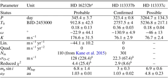
In this hypothesis, an activity cycle with a duration approxi-mating that of the candidate planet c period would explain both the FWHM and BIS long-term variations (and their correlation) as well as the RV long-term variations. We consider though that this interpretation has an important weakness: the RV corrected from the Keplerian fit of planet b only and the FWHM are not correlated (Pearson’s coefficient <0.1, see Figs.D.1and3). This is due to the RV and FWHM long-term variations being signifi-cantly shifted in phase (considering a period of ∼3265 days from the two-planet Keplerian fit). A phase shift of 15 to 30◦_between

RV, BIS, and FWHM activity-induced variations can be expected in the case of short-term stellar activity linked to the stellar rota-tional period (see e.g.Santos et al. 2014;Dumusque et al. 2014, who show that an active region crossing the visible stellar disk induces a RV shift and a line profile deformation with a slight phase shift). However, such a phase shift cannot be present in the case of a long-term activity cycle where the RV and line profile long-term variations are induced by the changing active region filling factor of the stellar disk along the cycle (Borgniet et al. 2015), being thus correlated (Dumusque et al. 2011). In the case of HD 113337, we derived the Pearson’s coefficient of the RV residuals of planet b versus FWHM while shifting in phase the FWHM along the ∼3265-day period deduced from the two-planet Keplerian fit (Fig.3). The highest correlation (∼0.65) is reached for a phase shift of ∼0.45 (or 1470 days), while the high-est anti-correlation (approximately −0.65) is reached for a phase shift of ∼0.7 (or 2290 days). While we still do not understand everything about stellar magnetic activity cycles, we consider that the observed shift between the RV and FWHM long-term variations is a strong argument against the activity cycle origin for the RV long-term variations, given our present knowledge (Dumusque et al. 2011). We note that long-period RV planets have already been distinguished from activity cycles by look-ing for the presence of a phase shift between the RV and the logR0

HKtaken as an activity proxy (Wright 2016).

Case of a faint binary. A faint, low-mass stellar compan-ion to HD 113337 in a (nearly) pole-on configuratcompan-ion could A87, page 5 of30

Fig. 3.Top panel: HD 113337 RV residuals from the Keplerian fit of planet b only vs time (black dots) and HD 113337 FWHM vs time (green triangles, same scale as RV). The Keplerian fit of candidate planet c is overplotted to the RV residuals of planet b (red). The average FWHM (∼13.7 km s−1_{) has been set to 0 for clarity. Middle panel: FWHM vs RV}

residuals of planet b. Bottom panel: Pearson’s correlation coefficient of RV residuals of planet b vs FWHM for different FWHM phase shifts, considering a ∼3265-day period (black solid line). The actual Pearson’s coefficient (for no FWHM phase shift) is displayed as a black dot. be just bright enough to slightly blend the primary spectrum, and thus induce the long-term FWHM and (low-amplitude) RV variations. HD 113337 v sin i is quite low for a F6V spectral type (seeBorgniet et al. 2014), meaning that the system could

be seen inclined (assuming that the star rotates in the same plane as the planetary system). Furthermore, HD 113337 is host to a cold debris disk that is most likely also inclined (K. Su, priv. comm.). However, in such a configuration, the RV and FWHM companion-induced variations would also have to be correlated (see Sect. 3.3.11), which is not the case here. Moreover, given the ∼7 MJup minimal mass of the

sec-ond candidate companion, the system inclination would have to be lower than 3◦ _{to allow for an actual companion mass}

of ∼150 MJup, which makes it quite improbable statistically.

Stellar mass-luminosity relations (Baraffe et al. 1998) taken for an age between 120 and 500 Myr show that a com-panion mass of 150 MJup would translate into a contrast of

6 magnitudes with the primary in the H band, and so even greater in the V band. This would make the effect of the companion light on the primary spectrum completely negligi-ble (especially when using a reference built from the primary spectra for the cross-correlation). Thus, we find the hypothesis of a low-mass stellar companion difficult to support given the observations.

Case of planet c. The RV and FWHM long-term variations are phase-shifted, which is not coherent with a magnetic activity cycle (see above). Furthermore, if plotting the BIS versus the RV residuals of planet b (Fig.D.1, fourth row), we find a still nearly flat diagram with a linear slope of −0.14 ± 0.02 and a correla-tion coefficient of −0.29. These values are very close to those we find for the (RV, BIS) diagram (see above), meaning that the horizontal spread in the (RV, BIS) diagram (characteristic of the presence of a companion) may well be induced by more than one planet. On the contrary, the RV residuals of the two-planet fit plotted versus the BIS show a linear slope of −0.49 ± 0.05 and an enhanced anti-correlation (−0.44, see above), meaning that the remaining RV dispersion is likely induced by stellar activity. We consider that the presence of a second GP in the system is thus a very convincing explanation for the RV long-term vari-ations and the shapes of the RV and RV residuals versus BIS diagrams. The additional presence of a long-term activity cycle would then explain the long-term FWHM and BIS variations, and the anti-correlation present between the RV residuals and the BIS.

To conclude here, we decided to classify HD 113337 as a can-didate two-planet system (planet b being confirmed and planet c still a candidate).

Additional remarks. In addition to the SOPHIEobservations, we are carrying out a multi-technique study (optical interferome-try, disk imaging, and deep imaging of the outer environment) of the HD 113337 system. The aim of this study is to bring as many constraints as possible on the system characteristics (stellar fun-damental parameters, age, inclination, etc.) and to fully cover the companion (mass, separation) space. This will be the topic of a forthcoming, dedicated paper.

3.1.2. Giant planet around HD 16232

HD 16232 (30 Ari B, HIP 12184) is a F6V dwarf star around which Guenther et al. (2009) reported the detection of a sub-stellar companion of ∼10 MJup minimal mass, based on RV

observations. This companion was further characterized thanks to new RV measurements (for a total of 110 spectra; seeKane et al. 2015, hereafter K15). These authors made a new esti-mation of the companion’s orbital parameters, making it of planetary nature, and additionally detected a long-term linear RV trend likely induced by a distant stellar companion. The

Fig. 4.HD 16232 phased RV. RV from K15 are displayed as blue dots, while our SOPHIE RV are displayed as black diamonds. The data are phased along the orbit of HD 16232b according to the Keplerian fit of K15 RV in Table2(the corresponding best model is displayed in red). Keplerian+linear fit performed by K15 thus gives mpsin i =

6.6 ± 0.9 MJup, P = 345.4 ± 3.8 days, and e = 0.18 ± 0.11,

cor-responding to a 1.01 ± 0.01 au semi-major axis (sma) for HD 16232b.

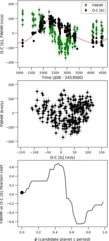
As part of our SOPHIEsurvey, we acquired 27 spectra on HD 16232, covering a 1893-day baseline. These data are enough to allow us to clearly see the long-term RV trend first detected by K15 in our SOPHIERV (Fig.D.2, third row). Furthermore, we find that the SOPHIEBIS versus RV diagram looks composite, with a horizontal spread indicative of a companion and a verti-cal spread induced by stellar activity and/or low-level pulsations. The SOPHIEBIS and FWHM do not show any significant sig-nal. We characterize the binary companion at the origin of the long-term RV trend in more detail in Sect.3.3.2. However, we do not detect any signal other than the binary-induced trend in our SOPHIERV (Fig. D.2, sixth row). This non-detection may be induced by our smaller number of observations compared to K15 and because our GP detectability is significantly degraded by the presence of the additional RV trend induced by the distant stellar companion. When plotting both RV data sets phased along the period from K15 (Fig.4), we find that our SOPHIERV and the best model from K15 are not in perfect agreement; however, it is unclear whether this is induced by a phase shift between our data and the fit or by the relatively high stellar noise in the data. If combining both RV data sets with yorbit, we do not achieve a good one-planet Keplerian fit. We note that we obtain a much better RV accuracy than K15 thanks to the use of SOPHIEand SAFIR. The Lomb–Scargle periodogram of the SOPHIERV is completely dominated by the window function, due to the pres-ence of the RV linear drift. On the contrary, the Lomb–Scargle and CLEAN periodograms of the more consequent K15 RV data set exhibit a clear peak at the planet period.

To investigate the impact of our temporal sampling on HD 16232b detectability, we computed the expected RV given K15 orbital fit at the epochs of our SOPHIEobservations. To do so, we extrapolated the Keplerian+linear fit from K15 to our observation epochs, and then added RV white noise with the same dispersion as the short-term (one night) RV jitter we obtained in our SOPHIERV data. These extrapolated RV look the same as our SOPHIERV, the RV linear drift being detectable, but not the planet-induced periodic RV variations (Fig. D.2, second row). Moreover, the Lomb–Scargle periodogram of the

extrapolated RV look very much the same as for our SOPHIERV (i.e. it is dominated by the window function), meaning that the GP detected by K15 is most probably non-detectable here, given our temporal sampling, our small number of observations compared to K15, and the level of short-term RV stellar jitter. Additional SOPHIEobservations sampled over the orbital period of HD 16232b could raise the ambiguity.

In the context of the following statistical analysis, we nonetheless decided to include HD 16232b as a strong can-didate GP. Based on the Keplerian fit by K15, we computed HD 16232b minimal mass considering a stellar mass of 1.2 Mto

be fully consistent with our stellar mass values, finding a slightly increased mpsin i = 6.8 ± 1.4 MJup. We include the detailed

parameters of the Keplerian fit in Table2. 3.2.θ Cyg: a system with complex RV variations

We detail here our results on HD 185395 or θ Cyg, a target that we observed extensively along our SOPHIEsurvey and that exhibits intriguingly complex RV and line profile variations. The RV and line profile data of θ Cyg are illustrated in detail in AppendixD.

The HD 185395 system. We presented our first results on θCyg (F4-5V, 1.37 M) inDesort et al.(2009, hereafter D09).

We made a first analysis of the RV based on 91 ELODIEspectra and our first 162 SOPHIEspectra. We showed in D09 that both

ELODIE and SOPHIEdata sets exhibit a strong quasi-periodic

RV signal, with a ∼220 m s−1 _{amplitude and a main}

periodic-ity of ∼150 days. Along with these RV variations was a flat (RV, BIS) diagram, the BIS variations being of much smaller amplitude (∼50 m s−1_{) than the RV. We argued in D09 that given}

the 7 km s−1 _{vsin i of the target, such a flat (RV, BIS) diagram}

would usually be a clear sign that the RV variations are induced by a planetary companion and are not of stellar origin. However, we also showed that despite this flat (RV, BIS) diagram, the BIS exhibits a strong periodicity of around 150 days, making the ori-gin of this periodicity puzzling. Furthermore, the ∼150-day RV variations could not be easily fitted with Keplerian models, with no stable and/or satisfying solution. We concluded in D09 that the origin of these complex RV and BIS variations could not yet be assessed. In addition, we reported the detection by imaging of a wide stellar companion to θ Cyg, that yet could not be respon-sible for the ∼150-day RV and line profile variations. θ Cyg was also independently followed in RV by another team (Howard & Fulton 2016). Based on 223 RV measurements obtained at the Lick Observatory, these authors also detected the long-term RV drift, as well as the quasi-periodic RV variations at ∼150 days, that they deemed statistically non-significant.

Finally, θ Cyg has been a target of interest in optical and IR interferometry. Multiple VEGAobservations allowedLigi et al.

(2012) to make a first estimation of θ Cyg angular diameter. Furthermore, the unusually high jitter and a possible periodic variability in the squared visibility measurements led the authors to speculate on the presence of a low-mass, unseen close stellar companion as the possible source of the RV and interferomet-ric jitter. However, the more recent study ofWhite et al.(2013), based notably on IR closure phase (CP) measurements made with the Michigan Infrared Combiner (MIRC, Monnier et al. 2004) interferometer on CHARA, found no evidence for a close stellar companion to θ Cyg. Based on the CP, these authors derived upper limits on a potential companion brightness, and found that a companion would have to be fainter than the primary by at least 4.7 magnitudes in the H band between 0.2 and 0.4 au, and fainter by at least 3.4 magnitudes between 0.4 and 0.7 au. A87, page 7 of30

Using stellar mass-luminosity relations (Baraffe et al. 1998) for an age of ∼1 Gyr, this translates into upper masses of 0.3 and 0.5 M, respectively.

New SOPHIEdata. We acquired 164 additional spectra on θCyg from 2009 to 2016, raising the total number of SOPHIE spectra to 326, and extending the SOPHIE time baseline to 3482 days (∼9.5 yr). We display the main SOPHIE spectro-scopic observables in Fig.D.3. The new SOPHIERV data set show both a long-term drift of slightly quadratic shape as well as the quasi-periodic ∼150-day variations. The quadratic trend is probably induced by the wide stellar companion imaged by D09 (see details in Sect. 3.3.10). Once corrected from this quadratic trend, the remaining RV variations have a total ampli-tude of 275 m s−1 _{and a dispersion of 64.5 m s}−1_{. The RV}

Lomb–Scargle periodogram exhibits several peaks above the 1% FAP between 100 and 500 days, but only a single peak at 150 days remains when cleaning the periodogram from the window function (CLEAN, Fig.D.3).

HD 185395 BIS shows only low-amplitude variations (rms 12.5 m s−1_{), thus leading to a flat (RV, BIS) diagram, indicative}

of a companion. However, the BIS Lomb–Scargle periodogram exhibits a single peak at a 145-day periodicity (in agreement with D09) which is also present in the CLEAN periodogram. The FWHM shows periodic variations with a 207 m s−1 _total

amplitude (rms 38 m s−1_{), corresponding to a single peak at}

149 days on the FWHM periodograms. The amount of corre-lation between the RV corrected from the quadratic fit and the FWHM is low (−0.3), but slightly higher than between the uncor-rected RV and the FWHM (−0.2). Both the BIS and FWHM data can be fitted fairly well with a nearly sinusoidal model with yorbit, with periods of 144 and 148 days, respectively, and marginally compatible phases. Finally, we recall that θ Cyg does not show any chromospheric emission in the calcium lines (hlogR0

HKi = −4.82).

Origin of the RV variations. As already shown by D09, a purely stellar origin to the ∼150-day RV and line pro-file variations is unlikely. Given θ Cyg v sin i of ∼7 km s−1_,

the rotational modulation of stellar magnetic activity should induce RV-correlated BIS variability, which is inconsistent with the flat (RV, BIS) diagram. Stellar granulation is not known to induce such high-amplitude RV variations at such a long period, whereas magnetic activity cycles last much longer given our present knowledge (several years, seeBaliunas et al. 1995). Finally, most stellar pulsations (i.e. solar-like or γ Dor-type) happen at much shorter periodicities; Kepler data have revealed solar-like oscillations on θ Cyg, but no other clear pulsation pattern (Guzik et al. 2011).

A second hypothesis could be the presence of a close, unseen low-mass stellar companion, which was not explored by D09. Such a companion would be just bright enough to slightly blend the primary spectrum and induce the ∼150-day periodic varia-tion in both the RV and the line profile observables without sig-nificantly altering the CCF shape.Santerne et al.(2015) showed that under some configurations, such an unresolved double-lined spectroscopic binary (hereafter SB2) would produce only a very weak correlation between the RV and the BIS, making it looking like a planetary signal. However, these authors also emphasized that even in such configurations, the FWHM should still be cor-related to the RV, while here the θ Cyg RV-FWHM correlation is weak. In contrast, a more convincing example of a RV–FWHM correlation probably induced by a spectroscopic binary can be found for HD 191195 (Sect. 3.3.11). For masses between ∼0

(i.e. negligible compared to the primary) and 0.5 M, such a

companion on a (nearly circular) 150-day orbital period would have a sma between 0.6 and 0.7 au, respectively. This falls into the separation range covered by the interferometric detection limits (≤0.5 M) fromWhite et al.(2013). The H-band contrasts

provided by these authors may well translate into larger con-trasts in the V band (i.e. the SOPHIErange) that would exclude significant effects on the CCF and RV. While not conclusive, this is another argument against the stellar companion hypothesis.

Finally, the planetary (or multi-planetary) hypothesis was already well explored by D09, but with no satisfying results. We tried to fit various Keplerian models with yorbit to θ Cyg RV (from 1 to 4 planets, with/without trends) and considered the cases detailed by D09, but to no avail. Furthermore, we also considered the ELODIERV data set from D09, and the RV data set published byHoward & Fulton(2016). Both these data sets exhibit RV variations of ∼300 m s−1 _{amplitude with a periodic}

character at about 150 days. We also tried to fit these different RV data sets with yorbit, either separately or by combining them. However, we did not obtain a satisfying solution. Furthermore, the main ∼150-day RV periodicity seems rather variable on our timebase, going from ∼125 to ∼180 days if dividing our timebase in several slices (AppendixD).

In conclusion, we consider that the origin of θ Cyg mid-term RV variations cannot be definitely determined. The variability of the RV variation period, the similarity of the RV, BIS and FWHM periodograms and the flat (RV, BIS) diagram make it a truly puzzling case.

3.3. RV long-term trends and stellar binaries

In this section, we describe fourteen massive and/or distant com-panions that we confidently identified in our survey. Given our data, most of them must be spectroscopic binaries (SB), while the others are candidate SB. We proceeded in the same way as done and explained before in PaperIX:

1. we identified the companion presence based on various diagnosis – RV variations, flat (RV, BIS) diagram, CCF variability, RV-FWHM correlation;

2. we distinguished between double-lined (SB2) and single-lined (SB1) binaries based on the presence or absence, respectively, of CCF distortions and/or RV-FWHM correla-tion;

3. if possible, we fitted the RV with various models (linear, quadratic, or Keplerian) using both our SOPHIE data and, whenever possible, other RV data sets available in the lit-erature. We then explored the RV residuals looking for lower-mass companions;

4. for our targets with long-term (linear or quadratic) RV trends, we constrained the companion properties (mpsin i,

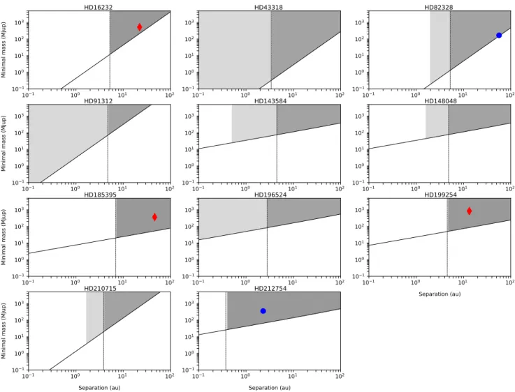
sma) given the available data, as we did in PaperIX. Briefly, we assumed the companion period to be at least equal to the observation time baseline, and the RV amplitude induced by the companion to be at least equal to the span of the observed RV trend, considering a circular orbit. We then deduced the corresponding minimal mass versus sma rela-tion (see PaperIXfor details). If appropriate, we looked for additional constraints from the literature.

3.3.1. HD 10453

HD 10453 (HIP 7916, F5V) shows high-amplitude (∼2.2 km s−1 _{peak-to-peak) RV variations over our 1590-day}

Fig. 5.Candidate binary companions (first part). From top to bottom rows: HD 10453, HD 20395, HD 43318, HD 82328, HD 143584. From left to right columns: RV time series, BIS vs RV, FWHM vs RV, stacked CCF. The best yorbit fit of the RV variations is overplotted in red to the RV. On the RV–FWHM diagram, the RV–FWHM correlation is overplotted in red if the absolute Pearson correlation coefficient is ≥0.6.

BIS and FWHM variations (Fig. 5) that are characteristic of a SB2 binary. We tried to fit the RV variations with yorbit using a Keplerian model. When letting free all the orbital parameters, the best model corresponds to a companion with mpsin i = 31.1 MJup, P = 249.2 ±20.5 days and e ' 0.76. However,

given the obvious SB2 nature of this companion considering the line profile variations, and that our temporal sampling far from covers the orbital phase of the binary secondary component, we consider that the actual companion mass has to be much larger than this estimation. We note that if running yorbit with various forced periods in the range of 100–3000 days, the solutions we find are almost as good as the free-parameter solution in terms of χ2_{, highlighting our incomplete temporal sampling.}

HD 10453 is a known binary. A stellar companion was resolved by speckle interferometry at a projected separation of ∼0.05” (∼2 au,Hartkopf et al. 2012) whileRiddle et al.(2015) imaged a stellar companion at a projected separation of ∼0.18” (∼7 au). Given the uncertainties on our orbital parameters, we cannot conclude whether the RV variations are induced by the companion detected by Hartkopf et al. (2012) or Riddle et al.

(2015), or whether the HD 10453 system has more components.

3.3.2. HD 16232

As presented in Sect. 3.1.2, we detect a long-term linear trend in our SOPHIE RV, along with a composite (RV, BIS) diagram indicative of a companion-induced trend (Fig.D.2). A linear RV trend was already reported byKane et al.(2015). To derive the best constraints on this companion, we combined our

SOPHIERV data set with the RV from K15 and fitted a linear RV

drift with yorbit. Such a combination of different RV data sets is possible as yorbit includes the RV offsets between the data sets as fitting parameters. The best solution is a linear trend with a −77.4 ± 3.2 m s−1_yr−1_{slope and a 802 m s}−1_{amplitude over the}

combined RV data set (Fig.6). The companion responsible for this RV trend has then to be more massive than 10 MJupand has

to be orbiting further out than 5.2 au (Fig.7).

A stellar companion to 30 Ari B has been imaged at a projected separation of ∼0.54” (∼22 au, Riddle et al. 2015, K15), with a mass estimated to be roughly 0.5 M (Roberts

et al. 2015). In addition, Kane et al.(2015) estimated that the mass of the imaged companion would have to be higher than 0.29 M(∼304 MJup) to explain the RV linear trend they detected.

Fig. 6. Targets with combined RV data sets. In all panels, RV data from our SOPHIE survey are plotted as black dots, and the yorbit fit we derived from the combined RV data sets (either linear, quadratic, or Keplerian) is overplotted in red. Top left panel: HD 16232 – RV data from Kane et al. (2015) are plot-ted as blue triangles. Top right panel:

HD 162003 – RV data from Endl et al.

(2016) are plotted as blue triangles. Bottom left panel: HD 185395 – our ELODIE RV data (Desort et al. 2009) are plotted as blue triangles and RV data fromHoward &

Fulton (2016) are plotted as orange

dia-monds. Bottom right panel: HD 199254 – our HARPS RV data (PaperIX) are plotted as blue triangles.

The mass and separation estimated byRoberts et al.(2015) for the companion they imaged are compatible with our constraints on the minimal mass and sma of the companion responsible for the long-term RV trend detected both in our SOPHIEdata and in K15 data (Fig.7).

3.3.3. HD 20395

HD 20395 (14 Eri, HIP 15244, F5V) shows high-amplitude (∼6.4 km s−1_{) RV variations along with a flat (RV, BIS)}

dia-gram, large variations in the CCF, and an apparent RV–FWHM anti-correlation (Fig.5) that are characteristic of a spectroscopic binary. We used the yorbit software to fit the RV variations. The best solution corresponds to a low-mass stellar companion with P = 675.2 ± 5.9 days, mpsin i ∼163 MJup, and e = 0.33 ±

0.02 (corresponding to a ∼1.7 au sma). However, given that our orbital phase coverage is not complete, we cannot exclude longer periods (and higher masses) for HD 20395B. If con-straining the companion orbital period to wider ranges (up to 2.104_–3.104 _{days) with yorbit, reliable orbital solutions can be}

found (with sma up to ∼15 au, mpsin i up to ∼350 MJup, and

eccentricities up to 0.8). HD 20395 has been reported as an astro-metric binary based on its proper motion (Makarov & Kaplan 2005; Frankowski et al. 2007), but without estimations of the orbital parameters.

3.3.4. HD 43318

HD 43318 (HIP 29716, F5V) shows a small (5 ± 0.7 m s−1_yr−1₎

long-term linear drift in its RV over our ∼1800-day timebase, along with a possibly composite (RV, BIS) diagram (Fig.5). We thus classify this trend as a candidate companion-induced one. When corrected from the linear trend, the RV residuals show a

dispersion two times smaller than the RV, and the Lomb–Scargle periodogram of the residuals show significantly less power at periods >100 days. Given the small amplitude of the RV trend over our timebase, the candidate distant companion can be either of GP, BD or stellar nature (Fig. 7). HD 43318 has not been reported as a binary before.

3.3.5. HD 82328

θ UMA (HIP 46853, F7V) shows a linear RV drift with a 78 m s−1 _{amplitude over our 3368-day timebase, which is best}

fitted with a long-term linear trend (Fig. 5). Assuming that the period of the companion responsible for the RV trend is at least equal to the total observation timebase, the companion can then be either of BD or stellar nature and has to be orbit-ing further than 5.3 au from the primary (Fig. 7). HD 82328 is a known physical binary with a ∼500 _{projected separation}

(Allen et al. 2000). Recently, Tokovinin (2014) has estimated the orbital parameters of the companion based on the absolute V-magnitudes of the components and assuming that the pro-jected separation corresponds to the actual sma of the compan-ion, finding P ∼ 322 yr and mpsin i = 0.16 M. Such a companion

is compatible with the detected RV trend (Fig.7). 3.3.6. HD 91312

HD 91312 (HIP 51658, A7IV) exhibits a large RV drift (of ∼4.1 km s−1 _{amplitude) over our 2635-day timebase (Fig. 8).}

As we cannot compute the line profiles for this target (too few spectral lines are available for SAFIRcomputation), we cannot check the (RV, BIS) diagram. Even so, we conclude that this RV drift is most probably induced by a companion because its ampli-tude is far larger than the short-term RV dispersion induced by

101 ₁₀0 ₁₀1 ₁₀2 101 100 101 102 103

Minimal mass (Mjup)

HD16232 101 ₁₀0 ₁₀1 ₁₀2 101 100 101 102 103 HD43318 101 ₁₀0 ₁₀1 ₁₀2 101 100 101 102 103 HD82328 101 ₁₀0 ₁₀1 ₁₀2 101 100 101 102 103

Minimal mass (Mjup)

HD91312 101 ₁₀0 ₁₀1 ₁₀2 101 100 101 102 103 HD143584 101 ₁₀0 ₁₀1 ₁₀2 101 100 101 102 103 HD148048 101 ₁₀0 ₁₀1 ₁₀2 101 100 101 102 103

Minimal mass (Mjup)

HD185395 101 ₁₀0 ₁₀1 ₁₀2 101 100 101 102 103 HD196524 101 ₁₀0 ₁₀1 ₁₀2 Separation (au) 101 100 101 102 103 HD199254 101 ₁₀0 ₁₀1 ₁₀2 Separation (au) 101 100 101 102 103

Minimal mass (Mjup)

HD210715 101 ₁₀0 ₁₀1 ₁₀2 Separation (au) 101 100 101 102 103 HD212754

Fig. 7.Constraints on the mpsin i and sma of the companions to our targets with RV linear or quadratic trends. Dark grey: possible (mass, sma)

domain for the companion given the available RV data, assuming a circular orbit and an orbital period at least equal to our total time baseline. Light grey: extended (mass, sma) domain in the case of orbital periods smaller than our total time baseline can still be considered, given the observation temporal sampling. Red diamonds: previously imaged companions from the literature: HD 16232 – DI fromRoberts et al.(2015); HD 185395 – DI fromDesort et al.(2009); HD 199254 – DI fromDe Rosa et al.(2014). Blue dots: companions previously detected with astrometry and/or RV from the literature: HD 82328 – astrometry fromTokovinin(2014); HD 212754 – RV fromGriffin(2010), and astrometry fromGoldin & Makarov

(2007) andTokovinin(2014).

stellar pulsations for this spectral type. This long-term RV drift is best fitted by a linear trend with a −566 ± 25 m s−1_yr−1_slope;

once corrected from the drift, the RV dispersion decreases from 1.75 km s−1_{to 415 m s}−1_.

HD 91312 is a known wide (2300 _{or ∼796 au) visual binary,}

which is dynamically linked according toKiyaeva et al.(2008). The very large projected separation of this companion makes it unlikely to be at the origin of the RV drift we detect. This RV trend is then likely induced by an unknown companion. Assum-ing an orbital period larger than our time baseline, this compan-ion has then to be of stellar mass and has to orbit further than 4.7 au around the primary (Fig.7). Interestingly, HD 91312 is still young (∼200 Myr) and shows an IR excess characteristic of the presence of a cold debris disk, according toRhee et al.(2007). A recent SED analysis (Rodriguez & Zuckerman 2012) gives a dust radius of 179 au; this could then be a circumbinary disk. 3.3.7. HD 143584

HD 143584 (HIP 78296, F0IV) exhibits high-amplitude (∼2 km s−1_{) RV variations over our 2596-day timebase on both}

) RV variations over our 2596-day timebase on both the short and long term, along with a composite (RV, BIS) diagram (Fig. 5). This is best explained by the presence of both a massive companion and stellar pulsations. The RV variations are best fit-ted with a long-term quadratic trend, even if periods shorter than our time baseline could still be possible. The dispersion of the

Fig. 8.HD 91312 RV time series. The assumed linear fit is overplotted

in red to the RV.

the short and long term, along with a composite (RV, BIS) dia-gram (Fig. 5). This is best explained by the presence of both a massive companion and stellar pulsations. The RV variations are best fitted with a long-term quadratic trend, even if peri-ods shorter than our time baseline could still be possible. The dispersion of the RV residuals is 291 m s−1_{, compared to the}

592 m s−1_{RV dispersion. Assuming an orbital period larger than}

our time baseline, the companion responsible for the RV long-term variations would have to be of stellar nature and would have to orbit further than 4.5 au from the primary (Fig.7). HD 143584 has not been reported as a binary before.

3.3.8. HD 148048

ηUmi (HIP 79822, F5V) exhibits long-term RV variations that are best fitted by a quadratic trend of 1600 m s−1_{amplitude over}

our 2988-day timebase. The (RV, BIS) diagram is composite with a horizontal spread induced by a companion and a vertical spread induced by stellar pulsations (Fig.9). Assuming an orbital period larger than our time baseline, the companion responsible for these RV variations would have to be of stellar nature and would have to orbit further than 4.8 au from the primary (Fig.7). HD 148048 has not been reported as a binary before.

3.3.9. HD 162003

ψ1 Dra A (HIP 86614, F5IV-V) shows high-amplitude (∼2 km s−1_{), long-term RV variations over our 2890-day time}

baseline, along with a flat (RV, BIS) diagram (Fig.9) characteris-tic of a companion. Furthermore, the RV and FWHM variations are strongly correlated (Pearson’s coefficient of 0.75), which make it a slightly SB2 binary.

HD 162003 has previously been reported as a spectro-scopic binary. Based on ∼40 RV measurements spanning over ∼1550 days,Toyota et al.(2009) detected a long-term RV trend of quadratic shape that they attributed to an unseen companion of mpsin i ∼ 50 MJup, with a sma lower than 140 au (assuming a

circular orbit) so that it remains on a stable orbit given the exis-tence of the wide binary ψ1 _{Dra B (HD 162004) at a projected}

separation of ∼3000_{(∼667 au) from HD 162003.Gullikson et al.}

(2015) detected this unseen companion (hereafter ψ1_{Dra C) by}

looking for a secondary peak in the CCF of HD 162003 spectra, in a way similar toBouchy et al.(2016). From this analysis, they estimated that ψ1_{Dra C had a mass of ∼0.7 M}

, making it of

stel-lar nature, and a sma of ∼9 au. Finally,Endl et al.(2016) directly detected ψ1 _{Dra C with speckle imaging on the one hand, and}

85 RV measurements spanning 15 yr (2000–2015) on the other hand, estimated the orbital parameters mpsin i ∼ 550 ± 5 MJup,

e = 0.67, and P = 6650 ± 160 days, corresponding to a ∼8.7 ± 0.1 au sma. We combined our SOPHIEdata with the RV from

Endl et al.(2016) and fitted a single Keplerian model to the com-bined RV data set with yorbit. Our best solution corresponds to a companion with a 661 ± 107 MJup minimal mass, a sma of

24.3 ±3.8 au and an eccentricity e = 0.87±0.02 (Fig.6). We con-clude that the RV variations that we detect in our SOPHIEdata are induced by ψ1 _{Dra C. However, the differences between}

our Keplerian model and the one derived by Endl et al.(2016) show that the sampling of the companion orbit is still not com-plete enough to adequately cover the period, meaning that large uncertainties still remain on its orbital parameters.

3.3.10. HD 185395

As presented in Sect. 3.2, we detect a long-term quadratic RV drift in addition to the RV mid-term complex variability of

θCyg. This specific RV long-term trend is induced by a distant companion, as shown by the flat (RV, BIS) diagram (Fig.D.3). To derive the best constraints on this companion, we combined our SOPHIERV data set to the RV acquired with ELODIEbefore (Desort et al. 2009) and to the RV data fromHoward & Fulton

(2016). This allowed us to expand the timebase to 5422 days (14.8 yr). Over the combined RV data set, the RV quadratic trend induced by the distant companion has an amplitude of ∼370 m s−1_{(Fig. 6). The companion responsible for this trend}

is then either of BD or stellar nature and has to orbit further than 7 au from the primary (Fig.7).

A distant stellar companion to θ Cyg was imaged byDesort et al.(2009) as a projected separation of 46.5 au from the pri-mary. Based on the measured contrast between the two compo-nents and on stellar evolutionary models, these authors deduced a mass of ∼0.35 Mfor the companion. These estimated mass

and projected separation are compatible with the constrains we derive from the RV long-term trend (Fig.7).

3.3.11. HD 191195

HD 191195 (F5V, 1.49 M) exhibits complex RV variations, with

a RV peak-to-peak amplitude of 272 m s−1 _{and a dispersion}

of 56.5 m s−1 _{(Fig. D.4). We consequently followed this}

tar-get intensively, acquiring 265 spectra over a 3191-day (∼8.7 yr) time baseline. The RV Lomb–Scargle shows multiple peaks between 100 and 103 _{days, but they are all aliases of a single}

∼300-day periodicity, as shown by the RV CLEAN periodogram. The BIS does not show high-amplitude variations (dispersion of 18 m s−1_{), hence the flat (RV, BIS) diagram. As did the RV,}

the FWHM exhibits high-amplitude (266 m s−1 _{peak-to-peak)}

complex variations. The FWHM Lomb–Scargle and CLEAN periodograms are strikingly similar to those of the RV, with a clear, single peak at ∼300 days in the CLEAN periodogram. We emphasize that HD 191195 RV and FWHM are strongly anti-correlated, with a Pearson’s correlation coefficient of −0.65 (Fig.D.4).

Given HD 191195 v sin i of 5.5 km s−1_{, the flat (RV, BIS)}

dia-gram points towards a companion as the source of the observed RV variability. We tried to fit single- or multi-companion Keplerian models to HD 191195 RV, including one to three planets and an additional linear or quadratic trend. However, none of them was able to reproduce convincingly the RV variations. We consider that this complex RV variability is induced by a faint stellar companion rather than by a plan-etary companion. This is strongly supported by the observed RV–FWHM anti-correlation, which can be explained by an unre-solved SB2 binary (seeSanterne et al. 2015, and the discussion about θ Cyg in Sect. 3.2). Given the relatively small v sin i of HD 191195, we might be seeing this possible binary system under an inclined or even close to pole-on configuration, which would explain such a low RV amplitude for a companion of stellar nature. HD 191195 has not been reported as a binary before.

3.3.12. HD 196524

β Del (HIP 101769, F5IV) shows high-amplitude (2 km s−1₎

RV variations over our 1179-day timebase, along with a flat (RV, BIS) diagram characteristic of a companion (Fig.9). The RV are best fitted by a quadratic model. Assuming an orbital period larger than our time baseline, the companion responsible for this RV trend would have to be of stellar mass and would have to orbit further than 2.8 au from the primary (Fig.7).

Fig. 9.Candidate binary companions (second part). From top to bottom rows: HD 148048, HD 162003, HD 196524, HD 210715, HD 212754. From left to right columns: RV time series, BIS vs RV, FWHM vs RV, stacked CCF. The best yorbit fit of the RV variations is overplotted in red to the RV. On the RV–FWHM diagram, the RV–FWHM correlation is overplotted in red if the absolute Pearson correlation coefficient is ≥0.6.

HD 196524 was already known as a spectroscopic binary (Pourbaix et al. 2004). Based on astrometric data,Malkov et al.

(2012) estimated its period to be of ∼26.7 yr, its eccentricity of 0.36, and its sma of ∼0.4400_{(∼13.6 au). At such a separation and}

given the mass constraints we bring, the companion would have a mass greater than ∼200 MJup(Fig.7).

3.3.13. HD 199254

We have already detected HD 199254 (HIP 103298, A5V) as a spectroscopic binary thanks to our HARPSRV (see PaperIX). We have also observed this target with SOPHIEand we detected a long-term, high-amplitude RV drift. When combining the

SOPHIE and HARPS RV data and fitting a trend model with

yorbit, we found the best solution to be a slightly quadratic trend of 923 m s−1_{amplitude over the total time baseline of 2400 days}

(Fig. 6). Given our combined RV data, the companion respon-sible for such a RV trend is of stellar nature and orbits further than 4.5 au from the primary (Fig. 7). A stellar companion

with properties compatible with these constraints was imaged around HD 199254 by De Rosa et al. (2014), see details in PaperIX.

3.3.14. HD 210715

HD 210715 (HIP 109521, A5V) exhibits a clear RV linear drift of 1.2 km s−1_{amplitude over the 1880-day timebase. Even if the}

(RV, BIS) diagram is dominated by a vertical spread induced by stellar pulsations characteristic of its stellar type (Fig.9), we con-sider that the RV long-term trend is induced by a distant massive companion.

HD 210715 has been reported as an astrometric binary (Makarov & Kaplan 2005; Frankowski et al. 2007), but no constraints on the companion parameters are available in the lit-erature. Assuming an orbital period larger than our time baseline, the unseen companion responsible for the RV long-term trend would have to be either of BD or stellar nature and would have to orbit further than 3.9 au from the primary (Fig.7).

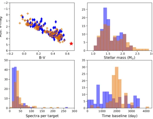
Fig. 10. Properties of our combined sample (SOPHIE +HARPS). Top left panel: position of our targets in an H–R diagram. Blue diamonds: SOPHIE targets; orange crosses: HARPS tar-gets. The Sun is displayed (red star) for com-parison. Top right panel: stellar mass histogram of our combined sample. Blue: SOPHIE tar-gets; orange: HARPS targets. Bottom left panel: spectrum number per target. Bottom right panel: timebase histogram.

3.3.15. HD 212754

We acquired only 19 RV measurements over 68 days on HD 212754 (HIP 110785, F7V), but we are able to detect a high-amplitude (2 km s−1_{) RV drift of quadratic shape, along with a}

flat (RV, BIS) diagram and large CCF variations that are indica-tive of a spectroscopic binary (Fig.9). Given our small timebase, we were not able to fully determine the orbital parameters of the companion. This companion has to orbit further than 0.4 au from the primary and is most probably of stellar nature (Fig.7), given the CCF variations.

HD 212754 is a known SB1 (Griffin 2010) and astromet-ric binary (Goldin & Makarov 2007) with an orbital period of ∼931 days, an eccentricity of 0.3–0.4 and a secondary minimal mass of 0.34 M (Tokovinin 2014) at a separation of ∼59 mas

(∼2.3 au). This already known stellar companion is most likely at the origin of the detected SOPHIERV variations.

4. Combined analysis of the SOPHIE+ HARPS surveys

Here, we combine our SOPHIE AF survey with the similar HARPSsurvey described in PaperIXto make a global analysis in terms of achieved companion detections, sensitivity and statis-tics in the 1- to 1000-day period range. In addition to the two GPs detected in this period range in this SOPHIEsurvey (HD 113337b and HD 16232b), we include the three confirmed GPs detected in our HARPSsurvey around two F6V targets (HD 60532b, c and HD 111998b) in the following analysis.

4.1. Characteristics of the combined survey

We combine the 125 AF dwarf stars of our SOPHIEsample to the 109 targets of our HARPSsurvey (PaperIX). We note that nine of our SOPHIEtargets were also part of our HARPS sam-ple: HD 13555, HD 25490, HD 29488, HD 102647, HD 197890, HD 199254, HD 211976, HD 218396, and HD 222368. Our com-bined AF sample is thus made of N = 225 distinct targets. In the case of the targets with both HARPSand SOPHIEobservations,

we selected the instrument for which we had the most RV data and the longest time span (i.e. we used the SOPHIE data for HD 102647 and HD 218396, and the HARPSdata for the seven other targets) and use the corresponding data in the following.

We do not combine HARPSand SOPHIERV data for these targets as it is not possible here to compute an accurate value of the zero-point between the two RV data sets, the SAFIRRV being relative RV. Furthermore, our detection limits are com-puted based on an analysis of the RV periodogram (Sect.4.3). In this context, a HARPS+ SOPHIERV combination might lead to a biased combined periodogram and thus biased detection lim-its. Hence, using only the RV data set with the most data and the longest time span ensures an unbiased periodogram, but it will lead to slightly more conservative detection limits. Our analysis of the combined survey is then based on 107 targets observed with HARPSand 118 targets observed with SOPHIE. The com-bination of these two samples is possible because we use the same target selection process (Appendix B). Both samples are thus very similar in terms of stellar physical properties (Fig.10). The median time baseline of our SOPHIEsurvey is 1448 days (mean time baseline 1640 days), with a median spectrum number per target of 23 (average 36) acquired during a median number of 11 visits (average 17). These values are lower than those obtained for our HARPSsample (see PaperIXand Fig.10). This differ-ence is mostly explained by the increased performance and better observing conditions of HARPS compared to SOPHIE. When combining the two surveys, we obtain a median timebase of 1888 days (average 1832) and a median number of 30 spectra acquired per target.

4.2. Stellar intrinsic variability

To characterize the stellar intrinsic variability of our targets, we display in Fig.11the RV dispersion (after having removed the companion-induced RV variations) and the mean RV uncertain-ties (accounting only for the photon noise) of our targets versus their main physical properties (B − V, v sin i, M?), as we did