Economics
Advances
Volume7, Issue 1 2007 Article8
Firm Size, Productivity, and Manager Wages:
A Job Assignment Approach
Volker Grossmann
∗∗University of Fribourg, [email protected]
Recommended Citation
Volker Grossmann (2007) “Firm Size, Productivity, and Manager Wages: A Job Assignment Ap-proach,” The B.E. Journal of Theoretical Economics: Vol. 7: Iss. 1 (Advances), Article 8.
Volker Grossmann
Abstract
Ability of managers and other nonproduction professionals is key for the productivity of firms. Hence, the assignment of heterogeneous nonproduction workers across firms determines the distri-bution of productivity. In turn, the transmission of productivity differences into profit differences – resulting from product market competition – determines firms’ willingness to pay for higher man-agerial skills. This paper explores the equilibrium assignment of nonproduction workers across ex ante identical firms which results from this interaction between product market and the market for nonproduction skills. The analysis suggests that, typically, large and productive firms coexist with small, low-productivity firms. Consistent with empirical evidence, a skewed distribution of firm size tends to arise. Moreover, the model predicts a positive relationship of firm size to productiv-ity, manager qualproductiv-ity, and manager remuneration. Finally, according to comparative-static analysis, higher intensity of product market competition can account for increases in the compensation at the top of the wage distribution.
KEYWORDS: asymmetric equilibrium, firm size, job assignment, manager wages, productivity
∗I am grateful to two anonymous referees, John Morgan (the editor) as well as to Christian Bayer, Johannes Binswanger, Josef Falkinger, Burkhard Heer and David Stadelmann for detailed com-ments on previous versions of the paper. Moreover, I am indebted for helpful discussions to Tomer Blumkin, Hartmut Egger, Armin Falk, Gilles Saint-Paul, Dennis Snower, John Sutton, Jian Tong, and seminar participants at the University of Southampton, the University of Zurich, the Econometric Society European Meeting (ESEM), the Annual Meeting of the European Economic Association (EEA), the Annual Meeting of the European Association for Research in Industrial Economics (EARIE), the Spring Meeting of Young Economists, and the CESifo Workshop on Employment and Social Protection in Munich. Financial support from EARIE associated with the Young Economists’ Essay Award received for an earlier version of this paper, entitled “Managerial Job Assignment and Imperfect Competition in Asymmetric Equilibrium”, is gratefully acknowl-edged. Author correspondence: University of Fribourg, Switzerland; CESifo, Munich, Germany; Institute for the Study of Labor (IZA), Bonn, Germany. Postal address: Volker Grossmann, De-partment of Economics, University of Fribourg, Bd. de P´erolles 90, G424, CH-1700 Fribourg, Switzerland. E-mail: [email protected].
1
Introduction
Managers and other nonproduction professionals in firms organize produc-tion, develop firm-specific know-how and design products, thereby determin-ing a firm’s productivity. Not surprisdetermin-ingly, empirical evidence from longi-tudinal microdata suggests that differences in both productivity and size of firms are driven by differences in manager quality (see e.g. the survey by Bartelsman and Doms, 2000). Moreover, there is a strong complementarity between skills and profitable innovations within firms (see Leiponen, 2005, and the references therein). This raises the question why large and produc-tive firms with highly-qualified nonproduction workers coexist with small, low-productivity firms.
This paper argues that such an asymmetric outcome naturally arises from the following interaction between competition of firms in monopolistic prod-uct markets and the market for heterogeneous nonprodprod-uction workers. On the one hand, assignment of nonproduction workers across firms determines the distribution of firms’ productivity. On the other hand, the transmission of productivity differences into profit differences — resulting from product market competition — determines firms’ willingness to pay for higher nonpro-duction skills.
It is shown that the equilibrium assignment of nonproduction skills, which results from this interaction, tends to be asymmetric when differences among firms in productivity become increasingly magnified in profit differences. That is, when gross profits of a firm are strictly convex as a function of its productivity, in equilibrium typically large and productive firms coexist with small, low-productivity firms — despite symmetry of potential entrants ex ante. Employing a specification where the price elasticity of product demand is constant (Dixit and Stiglitz, 1977), this property tends to arise when the price elasticity is sufficiently high and in line with observed price mark-ups.
In standard imperfect competition models, in which the number of active firms is determined by some exogenous entry cost, symmetry of potential en-trants typically leads to symmetric free-entry equilibria.1 A recent exception
is Yano (2006) who proposes a game-theoretic price competition model in which (a small number of) firms choosing a large-scale technology coexists
1For instance, see “love of variety” models of monopolistic competition (Spence, 1976;
Dixit and Stiglitz, 1977), “ideal variety” models (Lancaster, 1979; Helpman, 1981) or “location” (spatial) models (Hotelling, 1929; Salop, 1979).
with (a large number of) firms choosing a small-scale technology. In contrast, in the present paper asymmetry arises from firms’ hiring of nonproduction workers in general equilibrium rather than from technology choice.
The question why high-ability workers cluster in some firms and low-ability workers in others, and the implications for the distribution of firm size and the wage structure, have gained considerable attention (e.g., Kre-mer 1993; KreKre-mer and Maskin, 1996; Grossman and Maggi, 2000; Saint-Paul, 2001; Prat, 2002).2 The previous job assignment literature, by focussing on models with perfect product markets, suggests that asymmetric sorting of workers in firms is driven by technological complementarity and intrafirm spillovers among workers. In contrast, this paper argues that firm hetero-geneity arises from the incentive of firms to enter product market competition with high productivity. Intrafirm spillovers in the development of intrinsic firm characteristics are shown to contribute to the emergence of an asym-metric equilibrium, but are not necessary for its emergence.3
The paper aims to address a number of stylized facts related to the (asym-metric) assignment of key workers. Results are consistent with a positive relationship of firm size to productivity, manager quality, and wages of production workers. Also in line with empirical evidence, the sorting of non-production skills into firms tends to generate a skewed distribution of firm size (where size is measured by total employment in a firm). Moreover, al-lowing for multiple market locations, it is shown that high-productivity firms enter more market locations than low-productivity firms, i.e., have more es-tablishments. Finally, the analysis attempts to shed light on the dramatic shifts in the distribution of income in the U.S. and elsewhere. Evidence by Piketty and Saez (2003, 2007) suggests that particularly the share of wage income accrued to the upper decile of the wage distribution has increased. The proposed framework is particularly designed to address top wage in-come shares, due to its focus on high-skilled nonproduction workers. The
2For a comprehensive review of the less recent literature on job assignment, see
Sat-tinger (1993). Skewed wage distributions are usually derived from a magnification of skill differences into increasingly larger earning differentials. In seminal work on this idea, Rosen (1981) derives a strictly convex mapping from individual ability to individual earn-ings from the ability of more talented individuals (acting as atomistic firms) to cover a wider range of markets. In Rosen (1982), a similar magnification effect arises with respect to manager remuneration due to a complementarity between supervisory skills and the span of control.
3In contrast to the literature, such spillovers may occur among nonproduction rather
analysis suggests that higher intensity of product market competition leads to increases in the compensation at the top of the wage distribution.
Rather than stressing product market forces, Murphy and Zabojnik (2004) argue that technologically-driven increases in the demand for managerial skills which are transferable across firms and industries, relative to the de-mand for firm-specific skills, can account for the surge in top manager wages. Grossman and Maggi (2000) explore a perfect competition model in which, in line with the previous job assignment literature, workers with similar ability are matched together in firms if there is technological skill complementar-ity, whereas substitutability leads to cross-matching of workers. They show that in economies in which skills are relatively diversely distributed (like the U.S.) trade liberalization leads to wage increases for low-skilled individuals, whereas the effects on wages for the highest-skilled individuals are ambigu-ous.
The paper is organized as follows. Section 2 presents a basic model which is characterized by a specific product demand structure and technology. Sec-tion 3 analyzes the equilibrium assignment of nonproducSec-tion skills and dis-cusses the wage structure. It also examines whether the equilibrium job assignment is welfamaximizing. Section 4 derives comparative-static re-sults. Section 5 generalizes the basic model. Section 6 discusses the empirical relevance of the results. The last section briefly concludes.
2
The Basic Model
There is a continuum of identical market locations, indexed by m, which are represented as points in the unit interval. In each location m, there is a representative consumer whose preferences are reflected by utility function
Um = ⎛ ⎝ Nm Z 0 (xi,m) σ−1 σ di ⎞ ⎠ σ σ−1 , (1)
σ > 1, where xi,m is the quantity of good i ∈ [0, Nm] in market m. Measure
Nm is called the number of products in m.
There is a large number of identical potential entrants in the economy and entry is free. Opening up a firm may require to incur conventional fixed costs F ≥ 0. Let I = [0, I] be the set of firms which actually enter. There
are no flows of consumption goods across market locations, i.e., firms have to produce in each location the output they want to sell. In order to open an establishment in a single location, firms have to incur set up costs. These depend on the measure of market locations in which a firm decides to operate, called market range. Formally, let Mi ⊆ [0, 1] be the set of market locations
in which firm i ∈ I is active and let qi be the measure of Mi.4 Firm i’s
set up costs associated with a market range qi are given by Q(qi), where
Q(0) = 0 and Q(·) is both an increasing and convex function. Q and F may be interpreted as capital costs which are sunk when firms enter product market competition.
The analysis is confined to single-product firms. If firm i has an estab-lishment in m, it produces according production function
xi,m = αili,m, (2)
where li,m denotes i’s labor input in m. Productivity αi is the same for a
firm i in all markets m ∈ Mi.
There is a unit mass of individuals, endowed with one unit of labor, which they inelastically supply to a perfect labor market. Individuals are immobile across market locations. They differ in skill level h, like managerial quality or technical ability, relevant for the productivity of a firm. With respect to other tasks, labor is homogenous (as in Lucas, 1978, among others). Let g(h) be the mass function of the distribution of h, with support being the set H = {h1, h2, ..., hK
}, 0 ≤ h1 < h2 < ... < hK <
∞. Firms can perfectly observe h and workers seek the highest wage.
Firms hire an exogenous mass s > 0 nonproduction workers, called man-agers. The average skill level of these workers, ¯hi, determines productivity of
a firm in each market location.5 This reflects the idea that managers develop
common assets of a firm, which are applicable for all of its establishments.6
4More precisely, M
i∈ M, where M is a σ-algebra of Borel sets such that every element
is in the unit interval and qi is a Lebesgue measure.
5Taking the number of assigned workers in a firms as exogenous is a standard
assump-tion in the job assignment literature (e.g., Kremer 1993; Kremer and Maskin, 1996; Gross-man and Maggi, 2000; Saint-Paul, 2001; Prat, 2002). Certainly constituting a limitation, it contributes to the tractability of the analysis.
6In fact, empirical evidence suggests that productivity in single plants of a firm is
positively related to the average productivity of all other plants of this firm (Baily et al., 1992).
Formally, suppose
αi = a(¯hi), (3)
where a(·) is a strictly increasing function.
Firms are profit-maximizers and are engaged in monopolistic competition in each market location they are active. Production labor is chosen as nu-meraire good, i.e., the wage rate for production labor W = 1. As shown in Appendix A, with utility function (1) and production function (2), profits of firm i in m are given by
πi,m = li,m σ− 1 with li,m = (αi) σ−1Lm Ξm , (4) where Lm ≡ RNm
0 lj,mdj is the aggregate amount of production labor employed
in market m and Ξm ≡
RNm
0 (αi)σ−1di. As workers are immobile and of unit
mass, and since market locations are identical, in equilibrium, for all m, Lm = L = 1− sI.
The timing of events evolves according to the following stages, with de-cisions at each stage made simultaneously by firms.
• At stage 1, each firm i ∈ I hires managers with skills from the set H. Wage costs for nonproduction workers are sunk at later stages.
• At stage 2, firms decide in which markets to be active, i.e., each firm i∈ I chooses a set Mi ⊆ [0, 1].
• At stage 3, firms enter monopolistic product market competition. For instance, (productivity-enhancing) organizational or research activi-ties in firms take place prior to product market competition. Treating associ-ated wage costs for managers as sunk (stage 1) borrows from the IO literature on investment games which treats R&D and marketing outlays as endoge-nous sunk costs (e.g., Shaked and Sutton, 1982, 1983; Sutton, 1998). The model thus leads back endogenous sunk costs to individual characteristics, accounting for individual heterogeneity and observing resource constraints. The timing of events is also motivated by endogenous growth models in which technical change is driven by in-house R&D (e.g., Young, 1998), undertaken one period in advance of production and competition.
3
Equilibrium Analysis
For the equilibrium analysis of the basic model, we focus for simplicity on the case of two types of workers, K = 2, and specify
a(h) = h, Q(qi) = κ (qi) η
, (5)
where κ > 0 and η > 1. Section 5 analyzes a generalized model which does neither rely on these specifications nor on the specific stage 3 profit given by (4).
That η > 1 (i.e., a strictly convex shape of Q(·)) may be justified by logistic problems of firms to coordinate and govern single plants or branches, which may outweigh potential scale economies (e.g. Coase, 1937; Porter, 1986; Williamson, 1975). That function a is linear ensures that results on possibly asymmetric assignment of nonproduction workers to firms are not driven by intrafirm spillovers. Such spillovers could be captured by assuming that a is strictly convex. (See Remark 4 in section 5 for an elaboration and discussion in light of related literature.)
In equilibrium, as all firms maximize profits, each firm must have the same stage 3 profit, πi,m, in all markets it is located.7 Otherwise, there would be
‘arbitrage’ possibilities. Hence, in addition to Lm = L = 1− sI, we have
Ξm = Ξ, according to (4). This implies
πi,m=
(αi)σ−1
σ− 1 L
Ξ ≡ π(αi). (6)
Firms take aggregates L and Ξ as given at stage 2. We mostly focus on an interior solution for optimal market range qi, which maximizes qiπ(αi)−Q(qi).
(Remarks 1-3 discuss if and how the main results are modified when there are corner solutions.) Using (5), first-order condition π(αi) = Q0(qi)implies
qi = (π(αi)/κη)
1
η−1 ≡ q(αi). (7)
Thus, an important first result (generalized in section 5) is that firms with higher productivity (αi) have higher market ranges. This is because profits
7Suppose to the contrary that π
i,m > πi,m0 for m, m0 ∈ Mi. In this case, as market
locations are ex ante identical, there must be some firms which entered market m0 but not
m. However, this cannot hold in equilibrium when, as supposed, profits are higher in m than in m0. Thus, in equilibrium, π
per market location, π, are rising with αi. As αi = a(¯hi), specification a(h) =
h implies αi = ¯hi. Thus, stage 2 profits are given by f (¯hi) ≡ q(¯hi)π(¯hi)−
Q(q(¯hi)), called gross profits hereafter (as sunk costs for managers are not
included). Using Q(q) = κqη as well as (6) and (7), we obtain
f (¯hi) = η− 1 κη−11 µ L (σ− 1)ηΞ ¶ η η−1 (¯hi) (σ−1)η η−1 . (8)
3.1
Sorting in Equilibrium
We are now ready to derive the sorting of managerial skills into firms. For this, it is useful to first characterize the wage schedule, by relying on intuitive arguments. Rigorous proofs of the results in this subsection are provided for the generalized model in section 5.
As there is free entry, gross profits of a firm with average skill level ¯hi,
f (¯hi), must equal total wage costs for managers plus entry costs, F . That is,
net profits are zero and the average wage per manager is given by [f (¯hi)−
F ]/s. Firms take wages of managers, denoted by w(h) for skill type h ∈ H, as given (perfect labor market). As shown in section 5 (Lemma 2), if both skill types, h1, h2 are employed in the same firm, then the wage schedule is
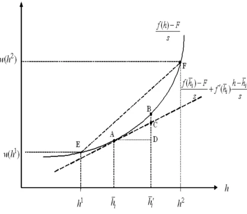
w(h) = f (¯hi)− F s + f 0(¯h i) h− ¯hi s , h∈ {h 1, h2 }. (9)
This can be seen intuitively. First, with this wage schedule, [f (¯hi)− F ]/s
is the average wage per manager, i.e., the requirement holds that net profits equal zero. Second, the equilibrium wage differential w(h2)
− w(h1)between
two types is proportional to the skill differential h2 − h1 whenever a firm employs both types as managers. This must be the case because productivity of a firm is determined by the average skill level of its managers.
If only one skill type h ∈ {h1, h2} is employed in a given firm, then w(h) = [f (h)− F ]/s is implied by free entry (zero net profits). If no firm hires more than one type of manager, the equilibrium job assignment is called hypersegregated, as there is complete segregation of firms by managerial skill. If all firms are identical in the skill mix they hire and thus their managers have the same average skill, equilibrium job assignment is called symmetric. It turns out that profit function (8) gives rise to a unique equilibrium with either hypersegregation or symmetry.
Proposition 1. (Sorting in basic model.) There exists a unique equilib-rium in which job assignment is hypersegregated if σ > 2−1/η and symmetric if σ < 2 − 1/η.8
Proof. Follows from Lemma 2 and Proposition 7 below (generalized model).
According to Proposition 1, if σ > 2 − 1/η, an asymmetric equilibrium with two types of firms necessarily arises, where firms differ in productiv-ity. The low-productivity firm hires only managers of skill h1 and the
high-productivity firm only managers of skill h2. This can be understood by the
intuitive properties of the wage schedule. Suppose to the contrary that there is a firm which hires both skill types as managers. If σ > 2−1/η, gross profits of firm i, f (¯hi), are strictly convex in the average skill level hired, according
to (8). In Fig. 1, wages w(h1) and w(h2) lie on the tangent (indicated by
the dotted line) of [f (h) − F ] /s at h = ¯hi (point A), according to (9). Now
suppose firm i would raise its average skill level from ¯hi to ¯h0i by replacing
some managers of type h1 by some of type h2 > h1. In Fig. 1, this leads to
additional average wage cost per manager of CD and to additional gross prof-its (net of F ) per manager of BD. As BD > CD, this means that, whenever firm i employs both skill types as managers, a profitable deviation exists. However, this contradicts the hypothesis that both types of skill are hired in equilibrium, since in equilibrium a profitable deviation must not be possible. Thus, if an equilibrium exists, it is unique and supports hypersegregation. It is also easy to see that the equilibrium with hypersegregation indeed exists. Under hypersegregation, zero profits command that wages w(h1) and w(h2)
are as depicted in Fig. 1. Given these wages, any deviation from hiring only skill h1 or only skill h2 means that average wage costs per manager are on
the line between points E and F and therefore would exceed gross profits (net of F ) per manager, £f (¯hi)− F
¤
/s, for any average skill level ¯hi ∈ (h1, h2).
Consequently, if f (h) is strictly convex, a profitable deviation does not exist for any firm under hypersegregation.9
Proposition 1 also provides an interesting insight for the emergence of
8We neglect the knife-edge case where σ = 2 − 1/η.
9Conversely, if f (h) is strictly concave, i.e., σ < 2 − 1/η, then under a symmetric job
assignment no profitable deviation exists for a single firm. That all firms must have the same average skill level in equilibrium follows from the fact (established in the proof of Proposition 7) that the wage schedule in a more profitable firm cannot be less steep than in a less profitable firm.
Figure 1: Equilibrium with hypersegregated job assignment.
segregation of firms by skill under monopolistic competition à la Dixit and Stiglitz (1977). In this framework, σ is the constant price elasticity of de-mand, as implied by utility function (1). If σ is high, then products are good substitutes such that monopoly power of firms is low, all other things equal. If σ is sufficiently high, such that f (h) is strictly convex, then a given difference in productivity among firms becomes increasingly magnified into differences in gross profits. Consequently, all firms have an increasingly stronger incen-tive to raise the average skill level of its managers. The transmission from higher product market competition to labor market competition breaks the ex ante symmetry among firms. As well known, the price mark-up (price over marginal costs) with constant price elasticity σ of product demand is
σ/(σ − 1). Empirical studies strongly suggest that the price mark-ups in manufacturing industries and in the private economy as a whole are quite small and clearly well below two (see e.g. Basu and Fernald, 1997, and the references therein). In the basic model, this means σ > 2, which is sufficient for hypersegregation, according to Proposition 1.
Remark 1. If there are strong scale economies in entering market lo-cations, Q is not necessarily convex. If we relax the assumption that Q is strictly convex, then we obtain a corner solution where all firms are active in all market locations, i.e., qi = 1 for all i. Whenever there is such a corner
solution, f (¯hi) = (σ−1)−1(¯hi)σ−1L/Ξ−Q(1), according to (6). Thus,
hyper-segregation occurs if and only if σ > 2 (f is strictly convex) and symmetry if and only if σ < 2 (f is strictly concave). Hence, the threshold intensity of product market competition which must be exceeded to obtain asymmet-ric sorting (σ = 2) is higher than the threshold σ = 2 − 1/η in the case where there is no corner solution for market ranges under the specifications in (5). Notably, however, in any case hypersegregated job assignment holds for empirically relevant price markups.
We know already that high-productivity firms are active in more market locations than low-productivity firms. If σ > 2−1/η, the market ranges of the two firm types are given by q(h1)and q(h2), respectively, where q(h2) > q(h1).
It follows that high-productivity firms also have larger size when firm size is measured by total employment (as often done in empirical studies). To see this, recall from (4) that, for a firm i, stage 3 profits in m are πi,m =
li,m/(σ− 1). The amount of labor employed by firm i in an establishment
is thus proportional to stage 3 profits and in equilibrium given by l(¯hi) ≡
(σ− 1)π(¯hi). Thus, clearly, the higher productivity αi = ¯hi of a firm is, the
more labor it employs in each establishment and thus also in total. Using l(¯hi) = (σ−1)π(¯hi)together with (6) and (7), we find that total employment
in firm i is given by lT otal(¯hi)≡ s + q(¯hi)l(¯hi) = s + µ (L/Ξ)η (σ− 1)κη ¶ 1 η−1 (¯hi) (σ−1)η η−1 . (10)
To establish the empirical relevance of the model (section 6), the following result (immediately implied by (10)) will be helpful.10
10The result also holds for the case where q
Proposition 2. (Firm Size.) If σ > 2, then firm size, lT otal(¯h i), is
increasing and strictly convex in ¯hi.
3.2
Does Equilibrium Job Assignment Maximize
Wel-fare?
The previous literature suggests that, under perfect competition, equilib-rium job assignment is efficient (e.g. Grossman and Maggi, 2000; Saint-Paul, 2001). The next result shows that this does not necessarily hold in the frame-work analyzed here. The welfare analysis is confined to the case where firms maximize profits at the product market competition stage. This ensures that a potential inefficiency of equilibrium is not driven by the well-known fact that output and prices, resulting from imperfect product market competition, are generally set at inefficient levels.
Consider a social planer which maximizes welfare by choosing, for the equilibrium number of firms, firms’ market ranges under both hypersegre-gated and symmetric job assignment (which are the two possible outcomes which can occur in equilibrium, according to Proposition 1), taking into ac-count subsequent monopolistic product market competition. The optimal job assignment pattern is found by comparing the two resulting welfare lev-els (one for hypersegregation, one for symmetry). Numerical analysis (the most relevant results are reported in Appendix B) suggests that the corre-sponding, maximal welfare level is typically higher than equilibrium welfare, for two reasons. First, given the equilibrium allocation of skills (hyperseg-regation or symmetry), market ranges are too low from a social point of view. That is, the number of products offered in each market location is too low, as consumers “love variety” in the analyzed model.11 Second, it may
be the case (although not necessarily so) that welfare is maximized under symmetry rather than hypersegregation, although the equilibrium job as-signment is hypersegregated (i.e., although σ > 2 − 1/η). Similarly, a social planer may prefer hypersegregation to symmetry, although the equilibrium job assignment is symmetric (i.e., although σ < 2 − 1/η). These insights are summarized as follows.
Proposition 3. (Welfare.) Consider welfare-maximizing job assignment case, lT otal(¯h
i) ≡ s + (σ − 1)π(¯hi), which is strictly convex in ¯hiif σ > 2, according to (6). 11Hence, clearly, if the social planer could affect costs to enter market locations, by
and market ranges for the equilibrium number of firms, given that firms max-imize profits at the product market competition stage. Equilibrium market ranges are generally not welfare-maximizing for a given job assignment. The equilibrium job assignment may or may not be welfare-maximizing.
The proof of this and all subsequent formal results are relegated to Ap-pendix B.
Remark 2. Contrary to the case where market ranges of firms are lim-ited, in a corner solution where qi = 1for all i, the equilibrium job assignment
is always efficient in the basic model. To see this, note that in the monopo-listic competition model of Dixit and Stiglitz (1977), with I goods and firms, utility function (1) implies that welfare, U , reads U = E/[R0I(pi)1−σdi]1/(1−σ),
where E = L + R0I(π(αi)− κ − F ) di is aggregate nominal income (use
W = 1 and Q(1) = κ) and pi = (1− 1/σ)−1(1/αi) is the price for good
i (see Appendix A). Using (6), Ξ =R0I(αi)σ−1di and L = 1 − sI, we obtain
E = (1− 1/σ)−1(1− sI) − (κ + F )I. Thus, combining p
i = (1− 1/σ)−1(1/αi)
with αi = ¯hi, for any firm number I, U is maximized if
RI
0 b(¯hi)di, where
b(h) ≡ hσ−1, is maximized. As b(h) is strictly convex if σ > 2 and strictly
concave if σ < 2, for any given mass of workers with skill h1 and h2, U is maximized under hypersegregation if σ > 2 and under symmetry if σ < 2. From Remark 1, we know that hypersegregation indeed holds in equilibrium if σ > 2 and symmetry prevails in equilibrium if σ < 2.
4
Comparative-Statics
Interestingly, starting from a symmetric equilibrium (which exists for a suffi-ciently low value of σ), the model is capable to generate the following result. If the price elasticity of demand σ increases such that the equilibrium becomes asymmetric, some firms may actually increase their size, lT otal, by attracting
better managers on average, while other firms see their size shrink. Thus, somewhat paradoxically, a higher intensity of product market competition, in the sense that the price elasticity of product demand becomes higher and thus price mark-up becomes lower, may give rise to the emergence of large, high-productivity firms in the first place.
The remainder of this section examines, for a given type of equilibrium (hypersegregation and symmetry), the determinants of both market ranges
of firms and wage dispersion between high- and low-skilled workers. In par-ticular, it addresses evidence on an increase in wages at the top of the wage distribution, typically earned by nonproduction workers like managers (see Piketty and Saez, 2003, 2007, further discussed in section 6). Two candidate explanations, both related to the intensity of product market competition, are explored: first, an increase in σ, reflecting lower price mark-ups, and second, a downward shift in κ, reflecting a reduction in institutional barriers to enter market locations.
As markets are symmetric ex ante, suppose the composition of firm types is the same at each market location in equilibrium. Also, to make the analysis interesting, the focus is on the case where both skill types, h1 and h2, are hired as managers. Intuitively and as shown in the generalized model, all high-skilled types are then employed as managers. Moreover, in a perfect labor market, a low-skilled manager receives the same wage as production workers, i.e., w(h1) = W = 1. w(h2) thus measures the wage premium for a
high skill.
Before examining this wage premium, the next proposition provides com-parative-static results for market ranges and the equilibrium number of firms, I. Market ranges are identical across firms in an equilibrium with symmet-ric job assignment. In an equilibrium with hypersegregated job assignment, they are given by q(h1) and q(h2) for low- and high-productivity firms,
re-spectively.
Proposition 4. (Market ranges). (i) In equilibrium with symmetric job assignment, the market range of firms is decreasing in κ. (ii) In equilibrium with hypersegregated job assignment, market ranges q(h1) and q(h2) are also
decreasing in κ. The relative market range q(h2)/q(h1) is increasing in σ
and independent of κ. (iii) The equilibrium number of firms ( I) is unrelated to κ under both hypersegregated and symmetric job assignment.
Proposition 4 is consistent with the notion that firms extend their market range if entry barriers to open establishments decline. For any given mar-ket range qi, a decrease in κ lowers both the absolute costs Q(qi) and the
marginal costs Q0(q
i) to enter market locations. Intuitively, an exogenous
decrease in Q would raise the number of firms, I. A decrease in Q0 would
increase market ranges and thereby, if Q remained the same, lower the num-ber of entering firms by reducing profits in each location. Taken together,
in the analyzed model, the equilibrium number of firms in the economy is unaffected whereas market ranges unambiguously increase. In an equilibrium where job assignment is hypersegregated, a decrease in κ implies that market ranges of high- and low-productivity firms increase in the same proportion such that the relative market range of the two types of firms, q(h2)/q(h1), is unaffected. In contrast, if the price mark-up decreases (increase in σ), productivity differences among firms become increasingly magnified in profit differences. This transmits into rising differences in market ranges among firms. Hence, q(h2)/q(h1)is increasing in σ.
We next turn to the effect of changes in σ and κ on the wage premium for a high skill, w(h2).
Proposition 5. (Wage inequality). Under both hypersegregated and symmetric job assignment, w(h2) is increasing in σ and unrelated to κ.
Although the result holds for both types of equilibrium (hypersegregation and symmetry), the intuition for the positive impact of an increase in σ (de-crease in price mark-up) on wage premium w(h2) is rather different across
the two types of equilibrium. If equilibrium job assignment is hypersegre-gated, an increase in σ implies larger magnification effects of differences in productivity on profit differences. This means that, after an increase in σ, a given relative skill h2/h1has a higher effect on the equilibrium skill premium,
as profits are related to manager wages.
In a symmetric equilibrium, the effect of a higher σ on w(h2) is more
subtle. According to (9) and w(h1) = 1, we have w(h2)
−1 = f0(¯h)(h2
−h1)/s,
where ¯h denotes the common average skill of the firms’ managers. A higher σ implies that ceteris paribus less firms are able to enter the economy, due to a first-order effect on stage 3 profits. A lower firm number I has two counteracting effects on wage premium w(h2). First, since less low-skilled
managers are hired, average skill ¯h increases, which means that marginal profit, f0, declines. (Recall from Proposition 1 that f is strictly concave in
a symmetric equilibrium.) This has a negative effect on w(h2). However, a
lower I ceteris paribus raises gross profits and under the specifications of the model also increases marginal profit, f0. This has a positive effect on w(h2),
which turns out to dominate the first effect.
In sum, the effect of a increase in the price elasticity of demand on the wage premium seems less robust in the case with symmetric firms than in the case with hypersegregation. However, the case with symmetric firms
is also the less relevant case from an empirical point of view, as discussed in section 3.1. In any case, one may conclude from the analysis that an increased intensity of product market competition which leads to lower price mark-ups has the potential to explain the observed increases in the premia for nonproduction skills.
In contrast, a decrease in barriers to enter markets, reflected by a lower κ, leaves the skill premium w(h2) unaffected. In the case of hypersegregation,
zero net profits in equilibrium imply that relative gross profits, f (h2)/f (h1), must equal relative sunk costs, (sw(h2) + F )/(s + F ). Since gross profits are
proportionally affected when κ changes, w(h2)does not change. In symmetric
equilibrium, as the discussion of the effect of a change in σ has suggested, w(h2) can only change in equilibrium when the number of firms, I, changes.
However, I is independent κ (Proposition 4).
Remark 3.12 In the case where all firms are active in all market locations (i.e., q(¯h) = 1 under symmetry and q(h1) = q(h2) = 1 under
hypersegrega-tion), w(h2)is again increasing in σ. With respect to the impact of a change
in κ, Proposition 5 does not hold. Since Q(1) = κ, a marginal change in κ is qualitatively similar to a change in sunk cost to open a firm, F , as mar-ket ranges cannot react if qi for all i. In this case, w(h2) is increasing in κ.
However, this result seems to be of minor interest.
5
Generalized Model
The central Proposition 1 in section 3 has been derived from intuitive rea-soning. This section provides a rigorous treatment, including the derivation of the wage schedule. It abstains from making specifications on functions a and Q and allows for more than two skill types, K > 2. Moreover, it works with profit functions at the product market competition stage 3 in a reduced form, rather than with (4).
In line with the analysis of the basic model, we require that the following holds. First, obviously, an equilibrium at stage 3 has to exist. Second, stage 3 profits of a firm are the same in any market location the firm is active (no arbitrage at stage 2). Third, differences among firms can be characterized by a single quality index, αi = a(¯hi), again called productivity, where stage 3
12The following claims can be proven in a way which is analogous to the proof of
profits of firm i are increasing in αi. Finally, if productivity or market ranges
increase for a non-zero mass of rival firms, stage 3 profits of a firm decline. More precisely, define a mapping z ≡ (α, q) which for each firm j gives us a pair (αj, qj); α: I → R+, j 7−→ αj; q: I → (0, 1], j 7−→ qj.13 We assume:
Assumption 1. For any z, there exists a real-valued function π( αi| z),
so that πi,m = π( αi| z) for all m ∈ [0, 1] if i is active in m, and π satisfies the
following properties: (i) ∂π( αi| ·)/∂αi > 0; (ii) for z = (α, q), z0 = (α0, q0),
we have π( ·| z) = π(·| z0) if α
j = α0j and qj = q0j for almost all j ∈ I, and
π(·| z) > π(·| z0) if α
j ≤ α0j and qj ≤ q0j with at least one strict inequality
holding for a positive mass of firms j ∈ I.
At stage 2, optimal market range q( αi| z) ≡ arg max0≤qi≤1{qiπ( αi| z) −
Q(qi)} is given by first-order condition
π( αi| z) ≥ Q0(qi), (11)
which is binding if qi < 1, i ∈ I.14 Note that q( αi| z) < 1 is possible only if
Q(qi) is strictly convex for at least some qi ∈ (0, 1].15 Given mapping α, in
equilibrium, the optimal choices of firms’ market range, leading to z, must be consistent with stage 3 profits under these optimal choices, π( αi| z). Denote
equilibrium profits of a firm i ∈ I at stage 2 (gross profits) by16
Π( αi| z) ≡ q(αi| z)π(αi| z) − Q(q(αi| z)). (12)
Proposition 6. (Gross profits and market ranges). For all i ∈ I, in equilibrium at stage 2, (i) ∂q( αi| z)/∂αi ≥ 0, and (ii) ∂Π(αi| z)/∂αi > 0.
Proposition 6 confirms in a more general way the result from the basic model that high-productivity firms do not only have higher gross profits
13In the basic model, mapping z has determined aggregate variables L and Ξ, which
have been taken as given by firms in their decisions at stages 1 and 2.
14Apply the Kuhn-Tucker theorem. Clearly, π( α
i| z) > Q0(0) and thus qi> 0 for a firm
i in any equilibrium, because otherwise a firm would not enter the economy in the first place.
15To see this, suppose to the contrary that Q(·) would not be strictly convex somewhere.
Then π( αi| z) ≥ Q0(1) and qi= 1 would hold. 16Note that Π( α
i| z) > 0 for all i ∈ I, according to (11), π( αi| z) > Q0(0), the convexity
˜ ˜
but also, if anything, wider market ranges than low-productivity firms. If Q(·) is strictly convex everywhere, then αi > αj implies qi > qj whenever
qj < 1. To derive more generally than in section 3 the conditions under
which in equilibrium firms may indeed differ in productivity αi, the following
auxiliary result will prove helpful. Lemma 1. (Convexity). If ∂2π( α
i| z)/∂α2i > 0 then ∂2Π( αi| z)/∂α2i >
0.
The firms’ decision problem at stage 1 is to hire a mass s of managers, which determines productivity, αi. First, define a class of “assignment
func-tions”
G≡ {g : H → [0, s] | ˜g(h) ≤ g(h) for all h ∈ H and X
h∈H
˜
g(h) = s}. (13)
(Recall that g(h) is the supply of workers with managerial skill h ∈ H in the economy.) ˜G describes the feasible hiring policies of a firm. At stage 1, each firm i ∈ I chooses an assignment function ˜gi ∈ ˜G. Depending on
this hiring policy, the average skill level of managers in firm i is given by ¯
hi = (1/s)
P ˜
h∈Hhgi(h). As αi = a(¯hi), the set of functions {g˜i ∈ ˜G| i ∈ I},
determines the mapping α. It is helpful to redefine gross profits as function of a firm’s average skill level ¯hi, i.e.,
f ( ¯hi ¯¯¯ z)≡ Π(a(¯hi) ¯¯¯ z). ˜ ˜ (14) There is an outside earnings option for all individuals not assigned as man-agers which is normalized to unity, W = 1. We are now ready to set up conditions for an equilibrium at stage 1. Equilibrium values are indicated by superscript (*).
Definition 1. (Equilibrium at stage 1). An equilibrium set of assignment functions {g∗
i ∈ G | i ∈ I}, together with a mapping w: H → R+ (wage
schedule), fulfills the following conditions: (a) Net profits are zero, i.e., for all i ∈ I, f ( ¯h∗i¯¯¯z∗) =X h∈H w(h)˜g∗i(h) + F, (15) where ¯h∗ i = (1/s) P ˜
h∈Hhg∗i(h) and z∗ = (α∗, q∗), with α∗i = a(¯h∗i) and
q∗
and for all i ∈ I, f ( ¯h0i ¯¯¯ z∗)≤ X h∈H w(h)˜gi0(h) + F, (16) where ¯h0 i = (1/s) P ˜
h∈Hhgi0(h). (c) For all h ∈ H, the following holds: w(h) ≥
1; if w(h) > 1, thenRi∈Ig˜∗
i(h)di = g(h); if
R
˜
i∈Ig˜∗i(h)di < g(h), then w(h) = 1.
Condition (a) of Definition 1 means that the sum of fixed entry costs F and the total wage bill for managers employed in a firm (i.e., endogenous sunk cost at stage 1) is equal to its gross profit, i.e., net profits of all firms are zero in equilibrium because of free entry. As potential entrants are identical ex ante, the only possibility for a firm to earn higher profits than other firms is to attract higher-skilled managers on average. Higher gross profits of a firm transmit into a higher average wage per manager of a firm. Condition (b) reflects that, at stage 1, each firm maximizes profits taking both z = z∗
and the wage schedule w(h), h ∈ H, as given. To motivate this, note that for any given wage schedule w(h), h ∈ H, no firm i wants to deviate from g∗
i ∈ ˜G (which leads to average skill ¯h∗i) if and only if
f ( ¯h∗i¯¯¯z∗)−X
h∈H
w(h)˜g∗i(h)≥ f(¯h0i¯¯¯z∗)−X
h∈H
w(h)˜gi0(h) (17)
for all alternative assignment functions ˜g0i ∈ ˜G(leading to ¯h0i). Inequality (16)
follows from (17) by using (15). According to condition (c), all h ∈ H from the potential pool of managers must at least receive the outside option, W = 1. (This implies that sunk costs at stage 1 are bounded from below by s+F .) Condition (c) also says that all workers of type h are employed as manager if their wage exceeds outside wage option W = 1. To motivate this, suppose w(h) > 1 andRi∈I˜gi∗(h)di < g(h). This means that there is excess supply for
nonproduction positions as workers seek the highest wage. However, this is inconsistent with a Walrasian equilibrium in the labor market. In contrast, if w(h) = 1 for some type h, then this type is indifferent whether or not to be assigned as manager.
We are now ready to derive the equilibrium wage structure. Define Si ≡
{h ∈ H : ˜gi∗(h) > 0}, the set of skill levels hired as manager in equilibrium
by firm i ∈ I. The set of skills assigned to nonproduction tasks reads Θ ≡ ∪i∈ISi. At stage 1, each firm i ∈ I chooses an assignment function ˜gi ∈ ˜Gby
maximizing net profits f ( ¯hi
¯¯¯
z)−Ph∈H˜gi(h)w(h)− F , taking as given z and
wage schedule as follows.
Lemma 2. (Wage schedule). In equilibrium, for all i ∈ I, (i)
w(h)≥ f ( ¯h ∗ i ¯¯¯ z∗)− F s + ∂f ( ¯hi ¯¯¯ z∗) ∂¯hi ¯¯¯ ¯¯¯ ¯¯ hi=¯h∗i h− ¯h∗ i s (18)
for all h ∈ Θ, with equality if h ∈ Si; (ii) there exists hk ∈ H such that
h ∈ Θ for all h ≥ hk and h /
∈ Θ for all h < hk; (iii) w(h) > 1 for all
h > hk; (iv) w(¯h∗ i) = £ f ( ¯h∗ i ¯¯¯ z∗)− F¤/s.
Lemma 2 confirms and generalizes the wage schedule discussed in section 3 for the basic model. According to part (i) of Lemma 2, within a firm, the wage schedule of managers is colinear. As already mentioned in the discussion of (9), this is an implication of the assumption that productivity of firm i, αi, depends on the average skill level, ¯hi, it hires. The right-hand
side of (18) gives the marginal benefit from hiring a nonproduction worker of type h for a firm with average skill level ¯h∗
i under the zero-profit condition
(15). Thus, in equilibrium, type h is not employed in such a firm if wage w(h) exceeds this marginal benefit. Part (ii) states that there exists an endogenous minimum skill level hk assigned as nonproduction worker and all individuals
with h > hk are hired as manager. According to part (iii), workers whose
skill exceeds hk have strictly higher earnings than their outside opportunity
in equilibrium (whereas w(hk) = 1if some workers of type hkare not assigned
as nonproduction worker, according to condition (c) of Definition 1). Finally, part (iv) states that any worker of type ¯h∗
i must obtain a wage rate equal to
the average wage per nonproduction worker in firm i (whether or not type ¯
h∗
i is actually employed in firm i).
Recall that an equilibrium job assignment is called hypersegregated if all firms hire a single skill type only and is called symmetric if average equilib-rium managerial skill, ¯h∗
i, is the same for all i ∈ I. Armed with the results
of Lemma 2, we can confirm Proposition 1 from the basic model, for an arbitrarily high number of skill types K, as follows.
Proposition 7. (Sorting). In any equilibrium, job assignment is hy-persegregated (symmetric) if gross profit function f ( ¯hi
¯¯¯
z∗) is strictly convex
(strictly concave) in ¯hi.
3, π( αi| ·), are strictly convex as function of αi (which holds for σ > 2 in
the basic model, according to (6)) and a(h) = h as assumed in section 3, then f ( ¯hi
¯¯¯
·) is strictly convex in ¯hi, according to (14) and Lemma 1. As
a result, and in line with Proposition 1, firms are completely segregated by skill in equilibrium. In turn, firms differ in gross profits and, possibly, in market ranges, according to Proposition 6. If the equilibrium job assignment is hypersegregated, wages of managers are related to gross profits according to w(h) = [f ( h| ·) − F ] /s, h ∈ Θ.
Remark 4. According to the preceding analysis, product market char-acteristics (reflected by stage 3 profits π( αi| ·)) are the driving force towards
asymmetry. One purpose of this paper (in addition to address important stylized facts, see section 6) is to demonstrate that asymmetric sorting can arise under empirically observed price markups and imperfect competition even in absence of technological complementarities (e.g. if a(h) = h). To see the relation to previous job assignment literature, which highlighted the role of technological complementarities for asymmetric job assignment equilibria rather than the role of the product market, consider the following pure labor market model. Let a¡¯hi
¢
now denote output of a homogenous (numeraire) good, produced under perfect competition, where ¯hi is the average skill level
of workers producing this good. (There are no nonproduction workers.) That is, in terms of the present analysis, f ( ¯hi
¯¯¯
·) ≡ a¡¯hi
¢
, F = 0 and W = 0. As argued in Saint-Paul (2001), in this model the case a00(·) > 0 leads to
sim-ilar results as the supermodular production function introduced by Kremer (1993). It has the interpretation that workers exert intrafirm spillovers on each other at all skill levels. According to Proposition 7, in such a labor market model, the way workers are sorted in equilibrium immediately fol-lows from the properties of production function a(·), i.e., hypersegregation (symmetry) occurs if a00(·) > (<)0. By design, only technology plays a role
for the sorting of workers.
The final result provides a sorting property which allows for the general case where the gross profit function is not strictly convex everywhere or strictly concave everywhere, i.e., there is not necessarily hypersegregation or symmetry in equilibrium.
Proposition 8. (General sorting property). In equilibrium, if ¯h∗ i > ¯h∗j
for some i, j ∈ I and hl
∈ Si, then h ≤ hl for all h ∈ Sj; moreover, if
¯
Although the context is different (see Remark 4), the result is in line with the labor market model in Saint-Paul (2001). It says that in any asymmet-ric equilibrium apart from hypersegregation, no skill level hired by a more productive firm can be lower than the highest skill hired by a less productive firm. Similarly, no skill level hired by a less productive firm can be higher than the lowest skill hired by a more productive firm. This implies that we can partition the set of skills hired as manager, Θ, into adjacent subsets and that firms which differ in productivity hire managerial skills from different subsets.
6
Relation to Stylized Facts
This section relates the implications of the analysis to five widely-recognized stylized facts.
1. Size distribution of firms. As frequently found in numerous studies, the size distribution of firms within industries is highly skewed.17 The predictions of the basic model are consistent with this observation. To see this, suppose strict convexity of stage 3 profits, and thus of gross profits, as a function of a firm’s productivity (Lemma 1). For observed price mark-ups, this is the case in the basic model (σ > 2). Strict convexity of profit functions gives rise to hypersegregation of the equilibrium job assignment (Propositions 1 and 7). Also suppose the mass function g(h), which characterizes the supply of manager skills, is decreasing for all h ∈ Θ (i.e., in the upper tale of the skill type distribution which contains the types hired as managers). That is, there are many mediocre and relatively few brilliant managers. Then, since firm size lT otal(h) of a firm which only hires managers of skill h is increasing in
h, the density function of firm size in the economy is decreasing (where size is measured by total employment). According to Proposition 2, as lT otal(h) is strictly convex, in addition, the firm size distribution function tends to be convex. Consequently, the firm size distribution tends to be skewed to the right.
For instance, suppose that g(h) is co-linear for h > hk, i.e. has the form
g(h) = β− γ · h, β, γ > 0. Denote the number of firms with firm size lT otal
by m(lT otal). According to (10), lT otal(h) has the form lT otal(h) = s + c· hυ with c > 0 and, if σ > 2, υ > 1. Define the inverse of this function,
˜
h(lT otal)
≡£(lT otal
− s)/c¤1/υ. Under hypersegregation, there are g(h)/s firms which hire only skill h > hk as manager. Hence, the number of firms with
size lT otal is given by
m(lT otal) = g(˜h(l T otal)) s = ˜β− ˜γ · £ (lT otal − s)¤1/υ, (19) ˜
β ≡ β/s, ˜γ ≡ γ · c−1/υ/s. Thus, m0(lT otal) < 0 and, as υ > 1, m00(lT otal) >
0. These properties prevail more generally whenever g(h) is decreasing and convex (or at least not “too concave”).
2. Firm size and productivity. Baily et al. (1992) find that the size of U.S. manufacturing firms is positively related to their total factor productiv-ity (see their Tab. 8 and 9). Moreover, Roberts and Supina (2000) report a negative correlation between marginal costs and firm size among U.S. manu-facturing firms. Our analysis consistent with empirical findings of a positive relationship between firms’ productivity and size (Proposition 2).
3. Sorting of managers. Evidence from matched employer-employee data strongly suggests that larger firms employ workers with higher aver-age skill levels (e.g., Abowd, Kramarz and Margolis, 1999; Troske, 1999). O’Shaughnessy, Levine and Capelli (2001) explicitly look at a measure for managerial skills, which is an index combining formal education with job requirements like problem-solving skills and predictability of tasks, known as ‘Hay points’. They find that average managerial skill levels substantially dif-fer across firms. This supports the asymmetric sorting hypothesis elaborated upon in this paper.
4. Firm size and wages. The analysis suggests that the higher the aver-age skill of manaver-agers in a firm i is, the higher are both the averaver-age waver-age per manager, [f (¯hi)− F ]/s, and firm size, lT otal(¯hi). Indeed, a positive
relation-ship between firm size and wages is a stylized fact (e.g., Abowd, Kramarz and Margolis, 1999; Troske, 1999). For instance, Troske (1999) controls for many firm-specific characteristics which have been suggested by economic theory on size-wage differentials, still finding a substantial impact of firm size on wages. A considerable part of this ‘size premium’ seems to be re-lated to imperfectly observable skills, like managerial talent, together with a clustering of skilled workers in large firms. Consistent with this explana-tion, O’Shaughnessy, Levine and Capelli (2001) find that their measure of managerial skills (‘Hay points’) is a good predictor for wages. Also at the CEO level, larger firms pay substantially higher salary (Conyon and Murphy,
2000).
5. Rising top wage income shares. Finally, Piketty and Saez (2003, 2007) provide evidence that the income share of the top decile of the U.S. pre-tax wage income distribution has increased dramatically in the last decades. For instance, whereas the top decile share of wage and salary income was 28 percent in 1980, it fairly gradually increased to 36 percent in 2000. Moreover, whereas average wage income increased only slightly in this time period, CEO pay has increased dramatically. According to Piketty and Saez (2007), average wage income of a full time-equivalent increased from US$ 33,023 in 1980 to US$ 38,846 in 2000 (in 2000 dollars). In the same time period, the average wage of the top 100 CEO’s increased from US$ 3.34 million to US$ 40.38 million.18 Conyon and Murphy (2000) show that manager wages have
surged recently also in the UK. Proposition 5 has addressed these important trends. It suggests that wage premia for nonproduction skills have surged as a consequence of increases in the intensity of product market competition which is reflected by a decrease in price mark-ups (increase in σ). Recent evidence by Cunat and Guadalupe (2006) supports the view that changes in the product market have affected the compensation at the top of the distribution. They find that an increase in foreign competition (captured by a firm-specific measure of import penetration) increases the remuneration of CEO’s in a firm and raises the reward for talent. That changes in product markets can account for the upward trend in manager remuneration until the year 2000 is an alternative to explanations which rest on technological changes (e.g. Acemoglu, 2002; Murphy and Zabojnik, 2004).
7
Conclusion
Ability of managers and other nonproduction professionals is key for the productivity of firms. Hence, the assignment of heterogeneous nonproduction workers across firms determines the distribution of productivity. In turn, the transmission of productivity differences into profit differences — resulting from product market competition — determines firms’ willingness to pay for higher nonproduction skills.
18The upward trend in wage payments at the top in the U.S. seems to have reversed
recently, however. Evidence suggests that the top decile wage income share has been 33.9 percent in 2002 (down from 36 percent in 2000) and the top 100 CEO’s earned on average “only” US$ 18.5 million (Piketty and Saez, 2007).
This paper has proposed a theory which suggests that the coexistence of large, high-productivity firms and small, low-productivity firms may derive from an asymmetric equilibrium assignment of nonproduction skills which results from this interaction. The analysis has shown that an asymmetric equilibrium assignment typically arises — despite symmetry of potential en-trants ex ante — when gross profits of a firm are strictly convex as a function of the firm’s productivity. In the monopolistic competition framework of Dixit and Stiglitz (1977), this property arises for observed price mark-ups.
It has been argued that the predictions of the model are consistent with a number of stylized facts: a skewed firm size distribution as well as a positive relationship of firm size to productivity, manager quality, and manager re-muneration. Comparative-static exercises suggest that observed increases in the compensation at the top of the distribution can be led back to a higher intensity of product market competition which is reflected by lower price mark-ups.
Appendix
A. Derivation of Equation (4)
Let Em be total consumption expenditure in m and pi,m the price for variety
i in market m. (1) implies that firm i faces in market m demand function xi,m =
Em(pi,m)−σ
RNm
0 (pi,m)1−σdi
, (A.1)
Firms take both aggregate expenditure Em and the denominator in (A.1) as
given when setting prices. With marginal cost 1/αi, we obtain the standard
mark-up price (Dixit and Stiglitz, 1977) pi,m=
1 αi
σ
σ− 1, (A.2)
i ∈ [0, Nm]. Using both equations (A.1) and (A.2), for any i, j ∈ [0, Nm],
xi,m/xj,m = (αi/αj)σ. Moreover, according to production function (2), we
Lm = RNm 0 lj,mdj = li,mα1−σi RNm 0 (αj)σ−1dj, which yields li,m = Lm(αi)σ−1 RNm 0 (αj)σ−1dj . (A.3)
Now use (2) and (A.2) to find that profit of firm i in m, πi,m = (pi,m −
1/αi)xi,m is given by πi,m = li,m/(σ− 1). This, together with (A.3), confirms
(4). ¥
B. Proofs
Proof of Proposition 3: We need to find welfare under both symmetry and hypersegregation for a given allocation of skills and market ranges. First, note that, with single-product firms, Rm∈[0,1]Nmdm =
R
i∈Iqidi holds. Let us
focus on the case where the firm composition is the same in each market and therefore Nm = N for all m. Thus, the number of products in each market
is
N = Z
i∈I
qidi. (A.4)
Moreover, substituting (A.1) into (1), welfare in each market (suppressing index m) is given by U = E/[R0N(pi)1−σdi]1/(1−σ). Expenditure E is equal
to nominal wage income of production workers, L (recall W = 1), plus total gross profits of firms net of F (being equal to manager wages under free entry). Thus, E = L + R0I(qiπ(αi)− Q(qi)− F ) di. Using (6) as well as
(A.2) and observing αi = ¯hi, we obtain
U = ⎛ ⎝L + I Z 0 ∙ qi(¯hi)σ−1 σ− 1 L Ξ − Q(qi) ¸ di− IF ⎞ ⎠σ− 1 σ Ξ 1 σ−1, (A.5)
where Ξ = R0N(¯hi)σ−1di. Denote by ˆg(h1) the mass of workers with skill h1
hired as manager. The mass of workers with skill h2 hired as manager is
equal to total supply of skill h2, g(h2). Thus, the equilibrium number of
firms in the economy reads
I = g(hˆ
1) + g(h2)
ˆ ˆ
Welfare under symmetry: The average managerial skill under symmetry is given by
¯ h = h
1g(h1) + h2g(h2)
g(h1) + g(h2) . (A.7)
Moreover, we have Ξ = N ¯hσ−1. In addition, (A.4) implies N = qI, where q
denotes the common market range of all firms under symmetry. Hence, using Q(q) = κqη in (A.5), welfare under symmetry, denoted by U
Sym, is USym = µ L− σ− 1 σ IF − σ− 1 σ κq η ¶ (qI)σ−11 ¯h, (A.8) ˆ ˆ
where ¯h is given by (A.7), I by (A.6) and L = 1 − sI.
Welfare under hypersegregation: Under hypersegregation, there are firms g(h1)/s firms which hire type h1 and g(h2)/s firms which hire type h2. De-note by q1 and q2 the market range of the former and the latter firm type,
respectively. Hence, according to (A.4), the number of products (and active firms) in each market location is
N = q
1g(h1) + q2g(h2)
s . (A.9)
In each location there is a share N/I of the existing firms. Using Ξ = RN
0 (¯hi)σ−1diwith ¯hi = h
1 for the ˆg(h1)/sfirms which hire type h1 and ¯h i = h2
for the g(h2)/s firms which hire type h2 we have
Ξ = N I µ ˆ g(h1) s (h 1)σ−1+g(h2) s (h 2)σ−1 ¶ . (A.10) ˆ ˆ
Substituting (A.6) and (A.9) into (A.10), we obtain Ξ = q 1g(h1) + q2g(h2) g(h1) + g(h2) µ ˆ g(h1) s (h 1)σ−1+ g(h2) s (h 2)σ−1 ¶ . (A.11)
Moreover, under hypersegregation,
I Z 0 qi(¯hi)σ−1di = ˆ g(h1) s q 1(h1)σ−1+ g(h 2) s q 2(h2)σ−1. (A.12)
hypersegregation, denoted by UHyp, is UHyp = σ− 1 σ Ξ 1 σ−1 Ã L + L Ξ ˆ g(h1) s q 1(h1)σ−1+g(h2) s q 2(h2)σ−1 σ− 1 − ˆ g(h1) s κ(q 1)η −g(h 2) s κ(q 2)η − IF ¶ , (A.13)
where Ξ is given by (A.11), I by (A.6) and L = 1 − sI.
Equilibrium market range q and firm number I under symmetry: Un-der symmetry, using Ξ = N ¯hσ−1, we obtain π(¯h) = (σ − 1)−1h¯σ−1L/Ξ =
(σ − 1)−1L/N. Optimality condition (7) implies q(¯h) = ¡π(¯h)/(κη)¢η−11 .
Substituting π(¯h) = (σ − 1)−1L/N into this equation, using N = qI as well
as L = 1 − sI, and solving for q, we obtain q = ∙ 1− sI κη (σ− 1) I ¸1 η (A.14) for the equilibrium market range under symmetry. We next derive ˆg(h1)and
thereby I. According to (9), we have sw(h) + F = f (¯h) + f0(¯h)(h− ¯h), h∈ {h1, h2
}. Using the expression for f(¯hi)in (8), this can be written as
sw(h) + F = f (¯h) ∙ 1 + (σ− 1)η η− 1 µ h ¯ h − 1 ¶¸ . (A.15)
Substituting Ξ = N ¯hσ−1 and L = 1 − sI into (8) and using N = qI together with the expression for q from (A.14), we find
f (¯h) = (η− 1)(1 − sI)
(σ− 1) ηI . (A.16)
Combining (A.15) and (A.16) implies w(h) = (η− 1)(1 − sI) (σ− 1) ηsI ∙ 1 +(σ− 1)η η− 1 µ h ¯ h − 1 ¶¸ −F s. (A.17)
use of the fact that w(h1) = 1, we find 1 = (η− 1) [1 − ˆg(h 1) − g(h2)] (σ− 1) η(ˆg(h1) + g(h2)) µ 1− (σ− 1)η η− 1 ¶ ˆ + 1− ˆg(h 1) − g(h2) h1g(h1) + h2g(h2)h 1 − Fs. (A.18) (A.18) implicitly defines ˆg(h1) under a symmetric job assignment in
equilib-rium.
Equilibrium market ranges and firm number under hypersegregation: Sub-stituting π(αi) = (σ− 1)−1(αi)σ−1L/Ξ into q(αi) = (π(αi)/κη)
1
η−1 from (7),
we find that q(h1)and q(h2) are given by
q(h1) = ∙ (h1)σ−1 (σ− 1)κη L Ξ ¸ 1 η−1 , q(h2) = µ h2 h1 ¶σ−1 η−1 q(h1). (A.19)
Observing that net profits are zero due to free entry and using w(h1) = 1,
we have f (h1) = s + F, where f (h1) = η− 1 κη−11 µ (L/Ξ)(h1)σ−1 (σ− 1)η ¶ η η−1 , (A.20)
according to (8). From (A.19), we get L/Ξ = (q(h1))η−1(σ− 1)κη/(h1)σ−1.
Substituting this into (A.20), condition f (h1) = s + F can be solved for q(h1)
to obtain q(h1) = ∙ s + F (η− 1)κ ¸1 η . ˆ (A.21) Now substitute (A.11) together with (A.21) and L = 1−sI = 1−g(h1)−g(h2) into the expression for q(h1) in (A.19). Then use q(h2) = (h2/h1)ση−1−1q(h1)
with q(h1) as given by (A.21) together with the fact that, in equilibrium, q1 = q(h1) and q2 = q(h2). This yields ˆg(h1), which is implicitly given by
(σ− 1)(1 + F/s)η η− 1 " ˆ g(h1) + g(h2) µ h2 h1 ¶σ−1 η−1# " ˆ g(h1) + g(h2) µ h2 h1 ¶σ−1# = £1− ˆg(h1) + g(h2)¤ £g(hˆ 1) + g(h2)¤. (A.22) Numerical results: The numerical results in Tab. 1 and 2 follow from the expressions derived, for the parameter specifications: F = 0.1, κ = 1, η = 4, h1 = 1, h2 = 2, g(h2) = 0.05. Variables with a ‘hat’ denote
welfare-maximizing levels. That is, ˆq1 and ˆq2 are the welfare-maximizing market
ranges of firms which hire only managers with skill h1 and h2, respectively, given that job assignment is hypersegregated. ˆq is the welfare-maximizing market range under symmetric job assignment. ˆUHyp and ˆUSym are resulting
utility levels. Variables without a ‘hat’ denote equilibrium levels.
I q USym qˆ1 qˆ2 qˆ UˆHyp UˆSym
s = 0.1 4.1 0.52 2.172 0.57 0.62 0.82 1.868 3.838 s = 0.6 0.92 0.71 0.154 0.64 0.76 0.81 0.211 0.206
Table 1: σ = 1.5 (symmetric equilibrium job assignment)
I q(h1) q(h2) U
Hyp qˆ1 qˆ2 qˆ UˆHyp UˆSym
s = 0.1 2.2 0.51 0.64 0.851 0.56 0.67 0.72 0.862 1.046
s = 0.6 0.59 0.70 0.88 0.263 0.78 0.92 0.71 0.269 0.234
Table 2: σ = 2 (hypersegregated equilibrium job assignment)
As η = 4, Proposition 1 implies that equilibrium job assignment is hy-persegregated if σ > 1.75 and symmetric if σ < 1.75. Tab. 1 and 2 show that equilibrium market ranges are too low from a social point of view un-der the equilibrium job assignment. Moreover, according to Tab. 1, which refers to σ = 1.5, if s = 0.6, then ˆUHyp > ˆUSym, although equilibrium job
assignment is symmetric. However, if s = 0.1, then ˆUHyp < ˆUSym,
show-ing that equilibrium job assignment may be welfare-maximizshow-ing (although equilibrium market ranges are not). According to Tab. 2, which refers to σ = 2, if s = 0.1, then ˆUHyp < ˆUSym, although equilibrium job assignment
is hypersegregated. However, if s = 0.6, then ˆUHyp> ˆUSym. This concludes
the proof. ¥
Proof of Proposition 4: Part (i). Equation (A.18) implies that ˆg(h1)
is independent of κ. Hence, from (A.6), also I is independent of κ. Using (A.14), this implies that in equilibrium q is decreasing in κ. This confirms part (i).
Part (ii). Since q(h2)/q(h1) = (h2/h1)ησ−1−1 and h2 > h1, q(h2)/q(h1) is
increasing in σ. Using (A.21) and q(h2) = (h2/h1)ση−1−1q(h1) from (A.19), we
find that both q(h1) and q(h2)are decreasing in κ. This confirms part (ii).
Part (iii): For the symmetric equilibrium job assignment, see the proof of part (i). For the hypersegregated equilibrium job assignment, (A.22) implies that ˆg(h1)and therefore I are independent of κ. This concludes the proof.¥
Proof of Proposition 5: The result is first proven for the hyperseg-regation case. In this case, free entry implies f (h1) = s + F and f (h2) =
sw(h2) + F. Hence, according to (8), ∙ f (h2) f (h1) = ¸ µ h2 h1 ¶(σ−1)η η−1 = w(h 2) + F/s 1 + F/s . (A.23)
Comparative-static results for the hypersegregation case follow.
For the symmetry case, substituting (A.6) and (A.7) into (A.17) and evaluating at h = h2, we obtain w(h2) = (η− 1)(1 − ˆg(h 1) − g(h2)) (σ− 1) η(ˆg(h1) + g(h2)) µ 1− (σ− 1)η η− 1 ¶ + ˆ 1− ˆg(h1) − g(h2) h1g(h1) + h2g(h2)h 2 −Fs. (A.24)
Using (A.18), this can be rewritten as
ˆ w(h2) = 1− ˆg(h 1) − g(h2) h1g(h1) + h2g(h2)(h 2 − h1). (A.25) ˆ ˆ
The right-hand side of (A.25) is decreasing in ˆg(h1)and independent of both
σ and κ. Moreover, recall from Proposition 1 that 1 > (σ − 1)η/(η − 1) must hold in the symmetry case. Hence, the right-hand side of (A.18) is decreasing in ˆg(h1). Applying the implicit function theorem to (A.18), we
thus find ∂g(h1)/∂σ < 0. In addition, ∂g(h1)/∂κ = 0. Using these facts
together with (A.25) confirms the result also for the symmetry case. ¥ Proof of Proposition 6: Part (ii) is proven first. If qi = q( αi| z) ∈