The Development of a Decision Support Software Application
to Improve Capital Equipment Management
by
Eric C. Selvik
B.S. in Mechanical Engineering Stanford University, 1993
Submitted to the Sloan School of Management and the Department of Mechanical Engineering in Partial Fulfillment of the Requirements for the Degrees of
Master of Science in Management and Master of Science in Mechanical Engineering
In conjunction with the Leaders for Manufacturing Program at the Massachusetts Institute of Technology
May 1999
@1999 Massachusetts Institute of Tec nology. ALL RIGHTS RESERVED.
Signature of Author - q
lMIT Sloan School of Management peartment of Mechanical Engineering May 15, 1999 Certified by
Professor Arnold Barnett MIT Sloan School of Management Thesis Supervisor Certified by
Associate Professor Duane Boning
MIT Department of Electri Engineering and Computer Science
Thesis Supervisor
Read by1
Rab-Stanley Gershwin, Senior Research Scientist
MIT Department of Mechanical Engineering Thesis Reader
Accepted by r - -
-Professor Ain Sonin Chairman, Committee on Graduate Students MIT)4epptment of Mechanical Engineering Accepted by
Larry Abeln, Director of Master's Program MIT Sloan School of Management
- w.15*'
The Development of a Decision Support Software Application to Improve Capital Equipment Management
by Eric C. Selvik
Submitted to the Sloan School of Management and the Department of Mechanical Engineering in Partial Fulfillment of the Requirements for the Degrees of
Master of Science in Management and
Master of Science in Mechanical Engineering
Abstract
A shift from a factory-constrained to a market-constrained business environment has driven Intel
to modify its operational focus to emphasize reduced costs, higher equipment utilization, and increased return on capital investment. Current methods of planning and managing factory
capacity have not been able to eliminate WIP bubbles and other operating inefficiencies that result in elevated costs and reduced predictable capacity.
A new Intel technique called the 80% Confidence methodology provides novel ways of
considering equipment availability by measuring and tracking the A80 Indicator, which is the 20e percentile of the daily average tool set availabilities. By focusing on the worst days of equipment availability, the A80 indicator represents a minimum availability that can routinely be expected, and therefore makes capacity planning more predictable.
This thesis describes the development of a Web-based software application, called the Equipment Management Improvement Tool (EMIT), that improves equipment management decisions by predicting equipment A80 availability given preventative maintenance schedules and basic
reliability parameters. It discusses the background, motivation, development methods, and results of the development, and illustrates one of many practical applications through a case study of the effects of a PM schedule change on A80 availability. The thesis offers suggestions for
improvements, and forwards future areas for extension of the application functionality. Thesis Supervisor: Arnold Barnett, Professor of Management Science
Acknowledgements
Hearty thanks are in order for my thesis advisors, Arnie Barnett and Duane Boning, who were very supportive, and instrumental in making my internship and this thesis a valuable and
enjoyable learning experience.
I would also like to thank all of the kind people at Intel Ireland who made my internship and this
thesis possible. In particular, I would like to express appreciation to Rick Babikian, Calum Cunningham, Brian Kelly, and Frank Daly for their ideas, support, direction, and effort. Special thanks to Helen, Martha, Timothy, Bernie, Karen and Maria for taking me in and making
breakfast my favorite meal of the day.
I would also like to acknowledge the support and resources made available to me through the
Leaders for Manufacturing Program, a partnership between MIT and major U.S. manufacturing companies.
I raise a toast to Arthur Guinness for his lovely pints of creamy stout that helped make the gray go away.... Slainte!
TABLE OF CONTENTS
ABSTRACT ... ... ---...-- - - - .3
ACKNOW LEDGEM ENTS... ...-- - - -. 4
1. INTRODUCTION AND BACK GROUND ... 7
1.1 THESIS OVERVIEW ... ... ---... 7
1.2 THESIS ORGANIZATION ...--.---.. ---... 9
1.3 HISTORY OF INTEL ...- - --- ----... 10
1.4 CURRENT BUSINESS ENVIRONMENT... 11
2. THE PROBLEM ...-...--- .. . ---... 14
2.1 VARIABLE OUTPUT AND W IP BUBBLES ... 14
2.2 THEORY OF CONSTRAINTS... ---... 15
2.3 CAPACITY CALCULATIONS ...---... ---... 16
2.4 THE A80 M ETRIC ...--. . ---... ... 20
2.5 W HAT IS A80 OR 80% CONFIDENCE?... . . . . . .. . .. . .. . .. . 21
2.6 BENEFITS OF A80 AND 80% CONFIDENCE M ETHODS... 22
3. TH E PROJECT ... ... ---... 24
3.1 PROBLEM STATEMENT ...---.. ---... 24
3.2 PROJECT OBJECTIVE...---... 24
3.3 PURPOSE...---... ... ... 25
3.4 PROJECT SCOPE AND DESIGN CRITERIA... ... 25
4. THE APPROACH ...- -... ----... 27
4.1 PRODUCT DEFINITION ...- ... -. - ---... 27
4.2 PRODUCT PLACEMENT ...- ... -... 28
4.3 DATA COLLECTION AND INTERPRETATION ... 29
4.4 DEVELOPMENT SOFTWARE SELECTION ... 30
4.5 M ODEL ASSUMPTIONS...---... 31
5. THE RESULT: EQUIPMENT MANAGEMENT IMPROVEMENT TOOL ... 33
5.1 SUMMARY OF KEY FUNCTIONALITY ... ... 33
5.2 USING EM IT ... 34
5.3 INPUTS ...----.--.--.-.-... 35
5.4 DATA RETRIEVAL: DOWNTIME EVENT SORTING TOOL ... 36
5.5 HOw EM IT W ORKS ...---... ... 38
5.6 EXAMPLE...-- .... ---... 40
5.7 M ODEL OUTPUT...- 41
6. DISCUSSION ... .... ---... --.... ... 45
6.1 INTERPRETATION OF THE OUTPUT ... 45
6.2 W H Y 80% CONFIDENCE ... 46
6.3 TBF AND TTR: M OVING AWAY FROM M EAN STATISTICS ... 48
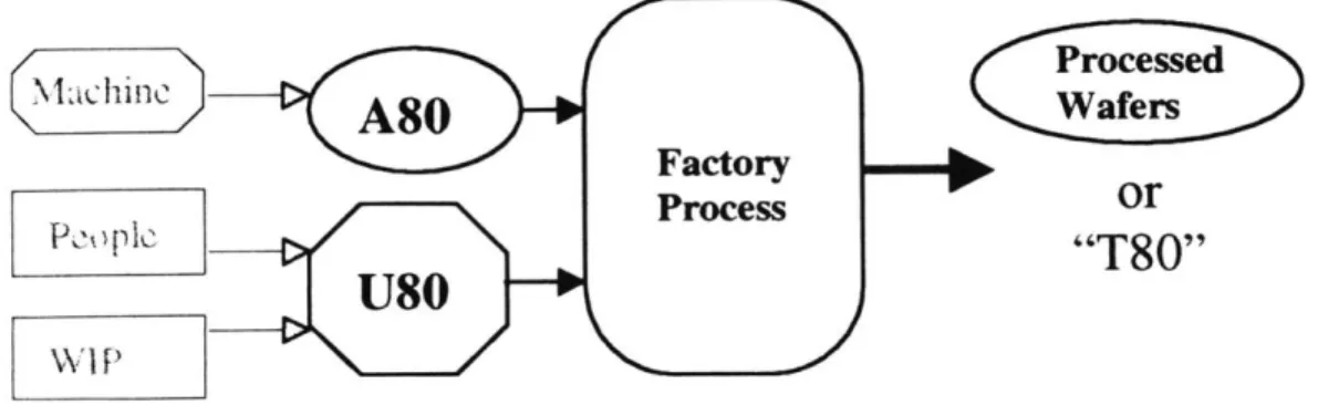
6.4 FuTURE CONSIDERATIONS: U80 AND T80... 49
7. RECOM M ENDATIONS ...----....- . --... ---... 52
7.1 APPLICATION IMPROVEMENTS... ... -.... ... 52
7.2 DATABASE AND ACCURACY IMPROVEMENTS ... 52
7.3 M ODEL GRANULARITY... ... - - - - -- - ---...53
7.4 USER INTERFACE IMPROVEMENTS ... 53
7.5 DATA ACQUISITION IMPROVEMENTS...54
7.7 OTHER POTENTIAL FEATURES ... 55
8.0 SUM M ARY ... ... 56
APPENDIX A: CASE STUDY OF PM POLICY CHANGE ... 58
A .1 SIMULATION SET UP ... 58
A .2 SIMULATION RESULTS ... 59
A.3 DIscusSION ... 60
1.
Introduction and Background
1.1 Thesis Overview
The shift from a factory-constrained to a market-constrained business environment and the drop in prices for PC microprocessors has eroded the incredible profitability that Intel has achieved for many years. In its effort to maintain its high profit margins on products while ensuring quality and delivery, Intel has endeavored to find areas for cost reduction and increase in return on assets. Given that Machinery and Equipment account for 37% of Intel's total assets (1997 Intel Annual Report), it is no surprise that equipment management has become a prime focus area for
streamlining and improvement projects. For semiconductor manufacturers like Intel, equipment management decisions such as how much capacity to keep, how often to perform preventative
maintenance, how much inventory buffer to maintain, and what trade-offs to make between technology and manufacturability have become critical to maintaining competitiveness.
A recent technique for improving operations in equipment-intensive, high-volume manufacturing
is Intel's A80 Equipment Availability indicator and Methodology. Developed in 1994 at Intel's Fabl0 in Ireland, this methodology builds on the recognition that for high-volume manufacturing over long periods of time, predictable manufacturing performance is as important as high mean performance. The A80 indicator (or 80% Confidence) seeks to focus Intel's operations and capital equipment management on predictable equipment capacity by creating a new tool availability
metric by which equipment performance is measured. Now, instead of looking at average availability as a measure of the performance of a tool set, Intel looks at the A80 Indicator, a statistic which reports the 20* percentile of the daily tool group availability over a 28-day rolling period. The A80 statistic captures an indication of both the mean and the variation of the
availability of equipment. Therefore, striving to maximize A80 forces equipment management policies to consider both the elevation of the mean and reduction of the variation. By
concentrating on the A80 statistic, Intel ensures that 80% of the time a required level of
equipment is available for processing, and therefore has greater predictable capacity to efficiently manufacture product and meet customer demand.
This changed focus in measuring equipment availability and utilization has brought into question the methods used in planning and executing scheduled preventative maintenance (PM). It was realized that how you schedule the PMs for your tool set will have performance effects on A80 (your predictable capacity), while not necessarily affecting the average availability. It is possible, therefore, that bottlenecks are designed into the manufacturing system simply in how the
preventative maintenance is managed, resulting in WIP bubbles, lost throughput, and other operating inefficiencies. It is clear that new methods must be discovered to maximize A80 when managing the interplay of downtime events for capital equipment.
To address the complexities of equipment management decisions, a software application was developed that computes the expected A80 availability performance of capital equipment given basic inputs about the scheduled and unscheduled events that characterize the machine. The development project took place in Intel's Fab 10 in County Kildare, Ireland, from June through December 1998, and resulted in the introduction of the software application called the Equipment Management Improvement Tool (EMIT) to the Intel intranet.
This thesis describes the background, motivation, developmental process, and results of the development of the EMIT software application. The thesis also discusses recommended
improvements to the application, and suggests future functionality to extend the usefulness of the model.
1.2 Thesis Organization
The thesis is divided into seven chapters, followed by a case study described in an appendix.
e Chapter 1 provides an overview of the thesis, a brief history of Intel, and the motivation for
the project out of the current business environment.
* Chapter 2 discusses the problems surrounding machine unavailability and the methods of measuring and rating machine performance. A more in-depth introduction of A80 is offered, as well as examples of the potential benefits from this metric
e Chapter 3 describes the problem statement, objective, purpose, scope, and general motivation
for the project.
" Chapter 4 discusses the approach used to solve the problem, decision points in the
development process, and the assumptions imbedded in the resulting application.
* Chapter 5 provides a full description of the resulting software application, with discussion on the inputs, outputs, and how the application works.
* Chapter 6 discusses the interpretation of the output, addresses some of the potential weaknesses in the model, and offers some larger take-aways and visions for future consideration.
e Chapter 7 recommends improvements that can readily be achieved with the EMIT application,
* The Appendix A describes the set up and results of a sample use of the application in analyzing the potential effects on A80 availability that a change in PM policy will have.
1.3 History of Intel
Intel Corporation was founded in 1968 by Robert Noyce and Gordon Moore in Mountain View,
CA. Through well-known products such as the Pentium, Pentium Pro, Pentium II, and now
Pentium III, Intel has grown to become the world's largest semiconductor manufacturer. With nearly 80% of the world market, Intel is the undisputed leader in the production of
microprocessors.
Intel's first products were primarily memory chips and microcontrollers. In 1971, Intel produced the first microprocessor (named the 4004) and by the late 1980's the company was focused on the production of the microprocessor and other logic chips which provide the 'brains' inside of computers. As the personal computer market blossomed, so did the demand for faster, more powerful microprocessors. This increased demand for processing capability drove Intel to introduce new, more powerful and complicated processors through the accelerated development of circuit designs and fabrication processing technologies. For many years, Intel has maintained the dominant position in this market through carefully planned and controlled releases of new technology that has kept them constantly ahead of their competition. Their technological superiority also allowed them to maintain high profit margins on their products (58% gross margins), capitalizing on the premium that consumers where willing to pay for increased processing capability. Intel had long operated in a factory constrained business environment,
meaning that the demand for their products outweighed their capacity to produce, and that they could sell every chip they produced at a premium. Consequently, Intel was incredibly profitable.
For the years 1987 - 1997, Intel's closing stock price achieved a compound annual growth rate of
42% (from Intel website, www.intc.com). As depicted in Figure 1.1, 1998 marked the 12' consecutive year of record revenues for Intel.
Figure 1.1: Intel Net Revenues
30000 25070 26270 25000 2 20847 20000 16202 15000 1 100002 Z 5844 5000 -0 07 3127 -1907 1987 1988 1989 1990 1991 1992 1993 1994 1995 1996 1997 1998 Year
1.4 Current Business Environment
A recent change in the personal computer market has driven Intel to refocus its business
strategies. The emergence of a new market segment - the sub $1000 PC market - has left Intel vulnerable. This market uses lower performance processors than the high-end that Intel has
traditionally led the development in. Intel underestimated the significance and size of this market, and largely ignored it, choosing to move ahead with higher performance, more expensive
microprocessors for higher-end computers.
The emergence of this new market segment and a simultaneous downturn in the overall demand in the PC industry placed Intel in a market-constrained business environment, characterized by
oversupply of their high margin chips. This substantial change in the business environment requires a significant modification in the way Intel runs its business. Instead of excessive demand, Intel faces overcapacity. Instead of competing on technology, they are forced to
compete on cost. Gone are the days when the marginal revenue far exceeded the cost to produce a chip and nearly any expense could be justified for technological advances and increased output. Intel now faces steadily falling prices for personal computers that result in lower prices for
microprocessors. In order to compete in the new sub-1000 PC market and avoid losing a large percent of its market share to its competitors, Intel must significantly reduce the cost to
manufacture its chips. Specific implications of this objective are a reduced investment in capital equipment and more efficient and cost effective use of existing capital equipment. Furthermore,
costs can be reduced through improved WIP and inventory management and an increased focus on total cost of ownership and return on investment for all decisions, including equipment purchase, staffing, and factory loading.
This new frame of mind is a difficult cultural change for such a large company that for so long maintained a very different mental model of what it took to compete and succeed in the
semiconductor manufacturing industry. In the past, issues of manufacturability were routinely subverted to technological increases because the marginal cost to produce was always far below marginal revenue on each chip. This technological focus had strong influences on many
operational areas within Intel. Equipment purchase decisions, staffing decisions, and
improvement project selection were driven by technology issues, many times "to the exclusion of availability" and other manufacturability aspects.
This paradigm shift represents the high-level motivation for this thesis project - helping Intel make better decisions about how they manage their equipment in order to increase efficient use, decrease total cost of ownership, increase the return on investments, and better manage WIP and inventory.
2.
The Problem
2.1 Variable Output and WIP Bubbles
One of the major problems in manufacturing systems that increases costs and reduces efficiency is variable or unpredictable process output. At Intel's wafer fabrication facilities, one of the most visible results of unpredictable output is the formation of "WIP bubbles", large WIP build-ups that propagate through the manufacturing system. Figure 2.1 depicts a sample WIP profile snapshot from Fab 10, where the WIP level at each process step is shown normalized to the planned, or balanced level.
Figure 2.1: Inventory Profile
NWIPBubbles"
3 5000->% 4000 3000 C 2000 -1000 -10 04 -1000 - -- - - - -w' -2000 ---3000 -E -4000-0 1 2 3 4 5 6 7 8 9 10 11 12 13 14 15 16 17 18 19 20
Process Step
As depicted in the graph, the WIP bubbles cause the WIP profile to deviate considerably from the balanced condition. These WIP bubbles have many negative effects on the manufacturing
system, including increased throughput time for a lot that severely limits responsiveness to rapidly changing demand, slower detection of quality problems [Wein], and the need to keep excess capacity which amounts to higher capital equipment expenditures.
In addition, there are the less quantifiable but significant negative consequences of general chaos in the factory from over-stressed equipment and workers, and scheduling problems for both human and capital resources.
2.2 Theory of Constraints
At Intel, it is felt that predictability is a key to manufacturing success. Statistical process control
is used throughout to track processes and reduce process variability. Factories are designed and managed using elements of the Theory of Constraints, whereby the system is balanced with respect to the output of the bottleneck process.
The Theory of Constraints (TOC), developed by Eli Goldratt, forwards that within any system there is always at least one weak link that constrains the overall output of the system. The system can produce no more than the constraint (known as the bottleneck) can deliver, no matter how productive or efficient the other links in system operate. Therefore, in order to maximize the output of the system, it is imperative to identify the constraint and maximize its output.
In order to increase the throughput of a manufacturing system, Goldratt offers the following steps for Constraint Management:
1. Identify the system constraints
2. Exploit the constraint
3. Subordinate all other processes to the constraint.
4. Elevate the constraint
According to this theory, the proper amount of capacity at each process step can be determined to balance the manufacturing system by the constraint, thereby increasing throughput and
minimizing WIP. Despite using the Theory of Constraints to balance the factory throughput, Intel finds that WIP bubbles continue to propagate through their fabs, and in addition, the bottleneck seems to move among different processing steps.
The WIP bubble problem can, in general, be traced to an incomplete understanding of the
capacity of the fabrication system, and specifically the capacity at each of the process steps. One could argue that these WIP fluctuations would not occur if sufficient capacity were maintained at each step to deal with upstream variability in process output. However, semiconductor
manufacturing equipment is very expensive, with typical single tool prices of $500,000 to $3 million, and entire fab costs in the neighborhood of $5 billion. Given these hefty equipment costs and the current business environment of cost cutting, one must look carefully at the financial and operational trade-offs on carrying "burst capacity," or extra machinery to deal with WIP
fluctuations.
A more cost-effective approach is to try to optimize the capacity of the equipment already in place
and understand what the key variables are that affect the throughput performance of the system.
2.3 Capacity Calculations
When trying to understand the mismatch in predicted and actual capacity, an obvious place to start is to look at the method used to calculate capacity of a tool set or system. According to the Theory of Constraints, the identification of the system constraint and near constraints is
accomplished by finding the process steps that have the lowest capacity. Intel often designs factories so that the process step with the lowest capacity is that which has the highest cost or most technology intensive equipment. By setting the capacity of the factory by the capacity of the intended or designed constraint, Intel can determine the theoretical capacity needed at each of the other process stations in order to maintain a smooth WIP flow through the system.
Intel uses the following equation to calculate tool set capacity:
Capacity = (RR * U/A * Avail * 168 * #tools)/ (# step * LY) Where
RR = run rate in wafers per hour
U/A = utilization to availability ratio: time the machine is processing WIP/ time machine is ready to process WIP
Avail = tool set availability (%)
168 = hours per week of theoretical process time
# tools = number of machines in the tool set
# step = number of times a wafer is processed by tool set in mfg. process
LY = line yield (% of good wafers passed on to next process step)
In accordance with TOC, the U/A of the constraint tool set is set to 1.0 (100% utilization) in order to achieve the goal of maximizing constraint output (TOC Step 2: Exploit the Constraint). For non-bottleneck tool sets, a design U/A of 0.85 is used. This provides "protective capacity" to ensure that the processes upstream of the constraint will keep the bottleneck fed, and the downstream tools can easily handle the WIP processed by the bottleneck and move it quickly away from the constraint. (TOC Step 3: Subordinate non-constraints to the constraint)
Assuming for now that the U/A is fixed, the other variables in the capacity equation are
the process) Line yields are generally very high, with little variability, and there are many processes in place to continue to improve this indicator. The most impact in the capacity variation, then, comes from the availability.
The long-term average availability will vary depending on the downtime events that occur with the machine, which can be generally classified as scheduled, unscheduled, and non-scheduled events. Scheduled events are periods when the machine is not available for a planned reason, and would include time the machine is down for preventative maintenance, performance monitors, engineering testing, and scheduled qualifications. Unscheduled events are times of unplanned machine downtime, and include activities when the machine is in repair, is waiting for product, or is waiting for a technician. The non-scheduled downtime includes events like factory shutdowns and automation work. The non-scheduled downtime accounts for a very small percentage of the total machine downtime and for practical purposes can be treated like unscheduled downtime.
The availability statistic that is generally used to determine capacity is the long-term average availability:
Availability = Total tool uptime! total time
where uptime is the time that a tool is able to process WIP, whether or not it does so. The average availability is a good general indicator to determine total system output capabilities and long-term throughput expectations for equipment sets, systems, and factories. However, using the average availability implies that 50% of the time the equipment availability is below the expected level, which implies that half the time the tool set or system will not have the capacity level that was calculated. This "time insensitivity" of availability leads to problems with unpredictable
throughput, since one will inevitably have machine availability when there is no WIP to process, and one will not have machine availability when there is WIP. When one of these conditions
occurs, WIP backs up at process stations and causes WIP bubbles to propagate through the manufacturing system.
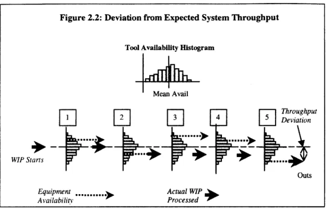
Figure 2.2 below illustrates this effect. A tool set might have an availability distribution like that
shown in the top of the figure. Consider a system of five tool sets with a variable availability that are balanced so that their average availability gives them sufficient capacity to maintain the desired throughput. A given amount of material is started based on the balanced factory capacity which is determined by the factory constraint. Even though the first machine has higher than average availability, only the WIP that was started is available to process, and so only that amount
is passed to the next tool set for processing. The second tool set experiences below average availability, and therefore only part of the WIP can be processed. The rest waits in a buffer in front of the process step. The third tool set is performing very well, but it is being fed only a fraction of the WIP it is capable of processing, and it can only process that which is passed to it from the upstream process. A similar circumstance occurs at tools set 4 and 5 where a below average availability day again reduces system output. We can see at the last station that the actual system output is well below the expected amount, and the throughput deviation can be traced to the machine availability mismatch with the WIP availability. In general, the downside variation reduces factory output, and upside variation is often lost elsewhere in the manufacturing system.
Figure 2.2: Deviation from Expected System Throughput
Tool Availability Histogram
Mean Avail WIP Siarts Equipment ,____,... Availability Outs Actual WIP Processed
2.4 The A80 Metric
Realization that the mean statistic was not robust in determining system capacity led Intel to begin
investigating new techniques to help mitigate the unpredictability problem. One such technique is Intel's A80 Equipment Availability Indicator and 80% Confidence Methodology. Developed in 1994 in Intel's Fabl0 in Ireland, this methodology seeks to focus Intel's operations and capital equipment management techniques on predictable equipment capacity by creating a new tool availability metric by which equipment performance is measured. This metric, known as the A80, calls attention to the days of low equipment availability, and seeks to improve equipment
2.5 What is A80 or 80% Confidence?
A80 is essentially a statistic representing the 20& percentile of the daily average availability data
of a tool set over a rolling 28-day period. The daily average availability is found by summing the
total uptime for all individual machines in a tool set and dividing by the total machine hours, which is the number of machines times 24 hours.
Daily Average = XAi where Ai is the daily availability for the ?'h tool in a set of n tools
Availability n * 24
For instance, a set of 5 tools might have a daily total of 100 hours of uptime, so the daily tool set availability would be
A = 100/5*24 = 86.6%
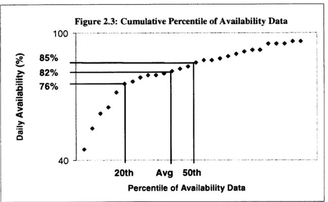
To find the A80 of a tool set, the daily tool set availabilities are listed in ascending order, and the 20* percentile of the data set is calculated (the sixth lowest availability). This is the availability at which one has 80% confidence that the tool set has performed.
For example, consider a 28-day period with the following daily tool set availabilities listed in ascending order, :
45,66,62,65,72,76,77,79,80,80,81,82,83,84,86,87,87,88,89,90,91,92,92,95,95,95,96,96
The A80, calculated as the 20 percentile of the data set is 76%, as shown in Figure 2.3. Also shown are the 50* percentile (85%) and mean availability (82%) of the data set for comparison.
2.6 Benefits of A80 and 80% Confidence Methods
By focusing on the A80 and achieving the 80% Confidence availability goals, Intel has found that
their tool performance is more predictable, and that WIP levels and system throughput vary less. Furthermore, the effort to increase A80 has led to a set of 80% Confidence Methodologies which have helped better utilize equipment and avoid some capital investment in increased capacity.
An example of an immediate benefit of the A80 analysis is the improved diagnosis of the constraint tool set in a manufacturing system. Consider the three tool sets illustrated in Figure 2.4. When comparing the mean availabilities, Tool C appears to be the bottleneck, and therefore one would subordinate the system to its throughput. One would also focus projects on improving
Figure 2.3: Cumulative Percentile of Availability Data 100 -85% _+++_ 82%, 76% cc 40 20th Avg 50th
the availability of this tool in order to increase system throughput (elevate the constraint). However, if the A80 statistic is compared, Tool A emerges as the constraint tool set, perhaps because Tool A has a high mean but highly variable availability and output. Using Tool A instead of the more predictable Tool C as the system constraint would have major changes in the
3. The Project
The equipment management challenges that erratic WIP levels invite, along with the general trend to cut costs and increase return on investment, necessitate the discovery and testing of new
equipment management methods to maximize A80 and improve equipment performance.
However, difficulties arise when trying to predict A80 availability. Percentile statistics are much less tractable than mean-based indicators, and require a more complicated approach to modeling and prediction.
In response to this need for a tool for analyzing A80 performance, the following project definition was established:
3.1 Problem Statement
There exists no tool for accurately planning and optimizing the interplay of downtime events for processing equipment when considering A80 availability. Current equipment availability
applications provide summary data on past equipment performance, but are not geared to forward-looking equipment issues such as preventative maintenance (PM) design improvement testing,
PM optimization, or equipment purchase decision inputs.
3.2 Project Objective
The objective of the project is to develop a software application that accurately models and predicts A80 equipment availability given basic reliability parameters. This tool will help to improve A80 equipment availability by assisting in the simultaneous management of machine maintenance activities and random machine failures.
3.3 Purpose
The purpose of the application is to deliver expected A80 equipment availability statistics based on equipment performance characteristics and PM schedules, and to predict the effects of equipment management policy changes on availability performance and WIP levels for systems of tool sets.
The information gathered using the application would be used in many ways. One important use is to discover and test new WIP and PM management methods to improve equipment availability. Another very practical use is to compare expected outcomes of candidate improvement projects to prioritize the highest-leverage activities, resulting in better use of engineering time. Also, the application output will enable analysis of factory capacity and inventory profiles to better understand interactions among systems of tools. Additionally, the application can be used analyze and compare expected equipment A80 performance when considering the purchase of new tools.
3.4 Project Scope and Design Criteria
To bound the project and provide some criteria to guide and motivate the development, the project scope was set by a few general guidelines. It was decided that the application should be
Windows compatible and/or a Web based platform for compatibility with current Intel IT norms. The target customer for the application was set initially as Intel internal, with possible extension to external customers. These target users for the application include Equipment Engineers, Manufacturing Engineers, Production Supervisors, the WIP Management Team, and the Capital Equipment Development Group. One last high-level criteria was that the application should be general enough to model any type of semiconductor processing or other capital equipment. This
would enable use by any equipment group within Intel, as well as the potential to develop the application into a new product for sale to other companies and industries.
4. The Approach
4.1 Product Definition
At the outset of the project, many key attributes for the product were undefined. Very little was understood about what exactly the software program should do, how it would work, what inputs and outputs were required, who the users would be, what their needs were, and how this product would fit with Intel's current suite of tools.
In order to understand what the needs were for such a product and put some definition on functionality and scope, extensive interviews were conducted with a wide variety of key constituents and potential users. The people interviewed included
e Equipment Engineers for Metal Etch, Planar, and CVD equipment groups
* Technicians for Planar equipment (on shop floor)
" Manufacturing engineer, Industrial Engineer
* Members of WIP management team
" Equipment Manager of Stepper supplier
e Equipment Engineer of supplier
" Functional Area Manager (Lithography)
e Manufacturing Engineering Manager
e Automation group engineer
" Process engineer, planar equipment
The interviews served the purposes of identifying the target user group and understanding the users' needs for a software tool, what inputs they would have available, and what outputs they would expect and find useful. Furthermore, it ensured that the development would produce a product that people would use, that did not duplicate existing applications, and that fit well with existing systems.
information, and easy processes for entering information into the model. Another important need was fast output, with no more than 10 minutes necessary to run a simulation. Of course, the model must be technically sound in order to be convincing enough to motivate changes. Finally, it was preferred that, as much as possible, the output be displayed in charts and graphs.
4.2 Product Placement
Another important consideration was how this particular software product would relate to existing tools used by Intel employees to model and analyze equipment availability information. There already existed the Improvement Engineering Applications (IEN Apps) that allowed engineers to analyze past data on equipment performance. These applications queried Intel databases and calculated availability statistics for any tool set in Intel's virtual factory, reporting the results in tabular and graphical format. Using these applications, employees could track equipment performance (average availability, A80, line yield) and monitor indicator trends.
There is another application at Intel that is used to model factory performance. It is a very
complicated discrete event simulator that models all facets of and transactions in the factory. This model uses as an input very specific information about the tool characteristic, equipment failures, PM schedules, run rates, as well as staffing schedules, technician ability level, and other detailed information about process variables. The output contains specific directions on optimal factory loading and staffing plans. However, this application is quite complicated, requires heavy
computing capability, is difficult to learn, and takes significant amounts of time to set up and run.
The proposed application seemed to comfortably fill the open space for a tool that provided A80 modeling capability, but that was quick, accessible, and easy to use.
4.3 Data Collection and Interpretation
Intel has a very well developed process control and data collection system called Workstream that controls and tracks activities that occur to every entity (wafer or tool) on the factory floor.
Furthermore, there are query systems that allow users to pull data and track tools over time. These provide a rich source of data for performing process and equipment analysis.
When analyzing data for the development of this product, one of the challenges was to interpret the data into actual events. If a query is run to look at all events for a tool when it is logged "down" (i.e. not available), the Workstream database will show many entries for one event. For
instance, if a tool fails and must be repaired, it must first be logged 'down to production', then logged in a repair state. The repair state might have several different repair entries and some nested testing states, and the tool might be logged in a waiting state for a part. When the tool is repaired, it might be logged into a different state in order to enter the information about the repair that was just completed. In this way, many entries describe one repair event, and this series of data entries varies significantly from event to event and tool to tool. Time was spent on the factory floor understanding some of the nuances of how the tools are actually logged on the floor. For instance, some technicians might follow a preventative maintenance routine exactly as is directed by the procedure. This might require performing an activity, returning to the
Workstream workstation to enter that the activity had been completed, and then reading the next activity, going back to the tool to complete that activity, and returning to the workstation to enter information about the completion of that particular instruction. Although this is the standard
frequently is time consuming and frustrating for technicians. Therefore, some technicians will perform several of the PM routines in succession, and then return to the workstation to enter in the completion information at the same time. These and other variable data input procedures create some challenges in trying to parse the data into descriptions of discrete events that are meaningful to estimating availabilities.
4.4 Development Software Selection
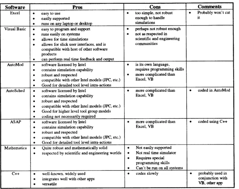
A key decision point was what type of software to use for development. As shown in Figure 4.1,
different software packages offered a range of pro's and con's. In the end, the customer
requirements and resource and time constraints dictated that a more simple software environment be used giving the advantages in ease of use and implementation. Another key benefit of using the simpler software was the ability to use previously written code which would save time and resources and allow easy integration into the current Improvement Engineering software application suite.
Figure 4.1: Software Environment Selection Matrix
Software Pros Cons Comments
Excel e easy to use e too simple, not robust e Probably won't cut
* easily supported enough to handle it
e runs on any laptop or desktop simulations
Visual Basic * easy to program and support e perhaps not robust enough * runs easily on systems e not as respected in e allows for time simulations scientific and engineering e allows for slick user interfaces, and is communities
compatible with host of other software products
e can perform real time feedback and output
AutoMod 0 software licensed by Intel e is its own language, * contains simulation capability requires programming skills * robust and respected * more complicated than e compatible with other Intel models (JPC, etc.) Excel, VB
* Good for detailed tool level intra-actions
AutoSched 0 software licensed by Intel * more complicated than e coded in AutoMod
0 contains simulation capability Excel, VB e robust and respected
" compatible with other Intel models (JPC, etc.) e Good for higher level tool group models * coding not necessarily required
ASAP * software licensed by Intel e more complicated than e coded using C++ e contains simulation capability Excel, VB
* robust and respected
* compatible with other Intel models (JPC, etc.) e Good for detailed tool level intra-actions
Mathematica e Quite robust and mathematically solid 0 Not easily supported * respected by scientific and engineering worlds e Not real time simulator
e Requires special programming skills * Can't be run on all systems
C++ 0 well-known. widely used a codes slowly * probably used in
e integrates well with other apps conjunction with
* versatile VB, other app
4.5 Model Assumptions
In order to simplify some of the complex variables that determine availability and throughput, the model starts with some basic assumptions. One is that the machines are independent, so that the availability of one is not affected by the availability of any other. It was assumed that there is uniform loading across the tool set, so that each machine in the group processes the same number of wafers per unit time. It was assumed that there is no correlation between Time Between Failure (TBF) and Time To Repair (TTR): the time it takes to repair a piece of equipment is unrelated to the amount of time since it was last repaired. Similarly, it was assumed that there is
no correlation between scheduled and unscheduled events, so that the occurrence of a scheduled event has no impact on the chances of an unscheduled event occurring, and vice-versa. Other assumptions include that the factory is in stead state, with constant wafer loading (e.g. 7000 WSPW), and that there is no prioritization of lots at any tool set.
Assumption 3, no correlation between TBF and TTR, is a key assumption for the basic operation of the application. Initial analysis of the data established that, for the Westech Planar equipment over the six month time frame, values of Time Between Failure and Time To Repair were uncorrelated. The data was analyzed using sample correlation coefficient analysis to determine
the coefficient of correlation,
px,y:
Px.y = cov(x,y1)
ax * y
where:
cov(x,y)= 1/n I(xi - x)(yi -
sy)
2 = 1/n I (xi - x)2
ay2= 1/n I (yi - y)2
For the Westech Planar equipment data, a correlation coefficient of px,y = -.019 was found
5.
The Result: Equipment Management Improvement Tool
5.1 Summary of Key Functionality
A software application was developed according to the project scope and customer input that
addresses the problem statement. The resulting application is called the Equipment Management Improvement Tool, or EMIT. This application predicts the A80 availability of a tool set given the preventative maintenance schedule and the statistical pattern of unscheduled downtime events of
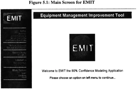
the equipment. Figure 5.1 shows the main screen for the application.
Figure 5.1: Main Screen for EMIT
Equipment Management Improvement Tool
Welcome to EMIT the 80% Confidence Modeling Application
Please choose an option on left menu to continue...
Using this application, an engineer can determine how changes in equipment maintenance routines and reliability parameters will affect the A80 availability of a set of tools. Furthermore,
the user can compare these expected outcomes among several projects, and thereby choose to work on the project that provides potential for the largest performance increase.
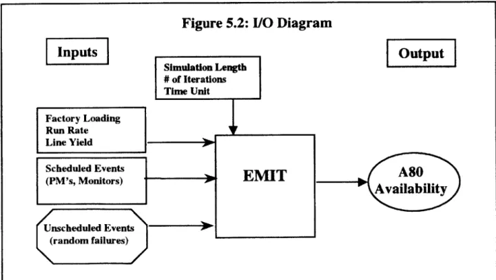
5.2 Using EMIT
The EMIT A80 module predicts the A80 performance for a defined machine group based on input
about the machines' scheduled and unscheduled downtime events. Figure 5.2 depicts the
Input/Output structure of the application.
Figure
5.2:
I/O Diagram
Inputs
IOutpu
Unscheduled Events (random failures)
5.3 Inputs
The inputs to the model are the following:
" Run Rate: the wafers per hour that a machine is capable of processing.
* Wafers visits per hour: the number of wafers expected to pass through the machine. This is a function of factory loading, yield, and the number of process steps the wafer sees at each machine.
* Machine PM schedules (scheduled events): input as a frequency, duration, and offset, where the offset is the number of hours from the beginning of the simulation that the first PM of this type occurs. A unique PM schedule can be entered for each machine, allowing for PM phasing across tool sets.
e Unscheduled Event Data: Time Between Failures (TBF), and Time To Repair (TTR),
uploaded from an Excel worksheet as strings of comma separated integers that are actual values of TBF and TTR from historical data on the machine. (Alternatively, the user can input a made-up distribution for each of these parameters). Both TBF and TTR values are found through querying Intel's database of operations data and separating out these
variables using an Excel worksheet (called the Downtime Event Sorting Tool, described below in Section 5.4)
* Simulation length: the number of hours over which the simulation should run (suggested
between 672 and 2016 hours = 1 to 3 months)
e Number of Iterations: number of runs of the simulation desired. Generally, the more
iterations run, the better characterization of the machine performance, but the longer it takes to complete the simulation.
A number of links in the Set Up menu on the left-hand side of the screen allow the user to input
the required information to run the simulation. In general, the user would use the following links to create and run a simulation of a tool set:
1. Machines: enter information about a machine (name, run rate, wafer outs, yield, etc.)
2. Scheduled Events links: enter frequency, duration, offset
3. Upload Unsch Data / Unscheduled Event Data: create unscheduled event profiles by either
uploading data or manually entering TBF and TTR distributions
4. Machine Sch Events / Machine Unsch Events: associate downtime events with specific machines
5. Machine Groups: group individual machines into tool sets
6. Simulation: enter simulation parameters, including Machine Group, length, and number of
iterations
7. Run Simulation: select and run a simulation
8. Simulation Results: view results of any previously run simulation
5.4 Data Retrieval: Downtime Event Sorting Tool
To pull data for the unscheduled events input, a complementary tool called the Downtime Event Sorting Tool was developed to support EMIT. It is a query application that allows the user to extract the necessary data about unscheduled downtime events needed to run the EMIT
application. The query is run and it collects data on the specified machines over a specified time period. This information is then entered into an Excel worksheet equipped with macros to help
sort the data for entry into the EMIT application. The worksheet is essentially a set of
"if/then/else" and logic algorithms that characterize the events according to certain parameters reported from the data query. The application classifies each event listing as Scheduled,
Unscheduled, or Other event type by looking at the description of the event and labeling it as S,
U, or 0 accordingly. Some examples of event classification types is shown below:
Unscheduled Scheduled Other
WAITING PART IN PM DEVELOPMENT
WAITING TECH SCHED QUAL AUTOMATION
WAITING PROD PERF MONITOR
IN REPAIR ENGINEERING
Based on the classification of Scheduled (S), Unscheduled (U), or Other (0), the amount of time spent in the logged event, and the start and finish times of each logged event, similar
"if/then/else" and logic functions group the individual logged events into discrete downtime events (DTEs). This is necessary since one discrete DTE can include many separate logged events, as described in Section 4.3. If a logged event marks the last entry for one discrete DTE, then it is designated as such. Knowing these designations allows the application to easily
determine the actual start and finish times of the discrete DTE. The application then adds up the time in event for each logged event to determine a total time in event for the discrete DTE, which is actually the Time to Repair (TTR) for that event.
Because the model characterizes events as either scheduled or unscheduled, it is necessary to remove time spent in a scheduled event (preventative maintenance) from the time in between unscheduled events in order to arrive at an actual TTR. The model already accounts for the time
in between failures spent in scheduled downtime, so this time should be removed from input data for the unscheduled downtime. An accompanying worksheet "purifies" the data by removing any
"scheduled" or "other" downtime that might have been included in the TBF for the unscheduled
events. After that, the TBF and pure TTR are saved in .CSV file, which is the appropriate file type for the EMIT application to upload.
5.5 How EMIT Works
When all the inputs are entered and the simulation is run, the application models equipment behavior by creating a virtual calendar for each tool in the set, and placing downtime events into
this calendar based on the event profiles defined by the user. The virtual calendar for a machine can be thought of as a time array where each element of the array represents the machine state for
one time unit of the simulation. Each element has three possible values: A, S, or U. A value of A in the array denotes a time unit that the machine is available to process WIP. A value of S or U indicates time when the machine is not available, but is instead down for a scheduled or
unscheduled event, respectively. Based on the user input for number of tools in the set, a corresponding number of such time array calendars would be created in the database.
When a simulation is run, the model goes through and populates the time array for each machine in the group modeled. The application first initializes the array so that all machine-hours are marked available (all integers in time array = A). Then, it places all of the scheduled events in the
time-array calendar for each machine. This is accomplished by changing the array elements from
A to S that correspond to the hours of scheduled downtime, as denoted by the frequency, duration,
Unscheduled downtime events are treated as random occurrences according to the distributions input for the Time Between Failures and the Time To Repair. A Monte Carlo simulator was developed that randomly selects among the unscheduled failure data that is extracted from the Intel database and uploaded into the application in the form of TBF and TTR values (in hours). This approach was chosen for a couple of important reasons. One is that using actual data preserves the mean and distribution of actual equipment performance. Also, the data can be extracted without much trouble, and takes no extra distribution modeling (i.e. trying to fit the data to a normal or other distribution).
In order to place the unscheduled events into the time array, the application goes to the
unscheduled events data and selects randomly from the TBF values. It then divides this number in half to get the number of available hours from the beginning of the simulation that the first unscheduled event occurs. A TTR value is then randomly selected, and the two numbers together define one unscheduled downtime event. For each unscheduled downtime event established through the random selection of the TBF and TTR values (g,h), the application counts g number of A's in the array corresponding to the TBF values, and changes the next h array values that equal A to U. Any array values that are already S or U are skipped over. This process is repeated until the length of the simulation is exceeded, for each machine, for each simulation run. Note: only the TBF for the first event in each simulation run is divided by 2; the rest use the actual TBF value randomly selected.
5.6 Example
As an example, let us assume that a machine has one preventative maintenance activity, a daily activity lasting two hours that is performed at 10 AM each day. The scheduled event therefore has the following parameters:
Frequency = 24 Duration = 2
Offset = 3 (the model is assumed to begin with the first shift at 7 AM)
Also, the machine has input data describing the unscheduled events that consists of the following two sets of 14 variables:
TBF 1, 77, 21, 4, 30, 9, 12, 2, 23, 8, 29, 45, 84, 2 7TR: 1, 22, 2, 13, 4, 5, 36, 53, 8, 1, 13, 41, 10, 9
Figure 5.3, below, shows how the application would construct and fill a time array to model
equipment with these input parameters.
The application will first place the scheduled event, changing the fourth and fifth, 28* and 29",
5 2"d and 5 3rd elements, etc. from A to S, until the full length of the simulation (as input by the
user) is filled. Then, in order to define the first unscheduled downtime event, the application would randomly choose a number between 1 and 14, say 7, corresponding to a TBF of 12 hours. Dividing this value by 2 for the first event gives a TBF of 6. Then, it chooses another random variable, say 11, which picks a TTR of 13. Given the unscheduled event (6,13), the model counts
out the first six available hours (skipping hours already marked 'down' for scheduled events) and blocks out the next 13 available hours, again skipping those already declared down for scheduled
activity. For this example, the 9* to 21" elements would be changed from A to U, as depicted in
to a TBF of 4 and TTR of 5 from the input data sets. Since this is not the first unscheduled event placed in the time array, the event (4,5) is placed by changing hours 26, 27, 30, 31, and 32 from A to U.
Figure 5.3: Example Simulation Time Array
Hou 112131
1.1 1 1911 ''11 11 11 11 11 12 12 12 1212121212 12ArrayValue AAAISSIAAIAUIUUIUU UUUUUAAAAUUS SJUUJUAJAAJAA AAJAAJA
Array Value:
A = available
S, U = unavailable for scheduled or unscheduled event
This process is repeated until the end of the time array for the machine is reached, and it starts for the next machine, which may or may not use the same TBF and TTR data.
5.7 Model Output
When all of the iterations of a simulation have been completed, the application calculates a daily average availability across the tool set. It counts the number of A's in all of the machine arrays for each 24 hour time block and divides by the daily number of tool-hours, which is equal to the number of machines in the tool set times 24 hours in the day. (So if we had chosen a length of 2400 hrs for the simulation, we would have 100 daily availability percentages stored for the tool set at the conclusion of the simulation). From this set of daily tool group availabilities, EMIT calculates the 20th percentile, rounds to the nearest integer, and stores the number as the A80
statistic for that iteration. All arrays are then reset, and this sequence is repeated for the number of iterations that the user directed the simulation to run. Therefore, the output of the simulation is a
The application reports the simulation output in a number of ways: tables, graphs, and lists of summary statistics of the simulated data. The simulation results are shown in Figures 5.4, 5.5
and 5.6.
Figure 5.4: Simulation Output - Avail Table
Simulation Results
Here are the simulation results...
Machine Availability Details
.01002 0030044 006 00~8,009,010 011'0120I13 01lt0150 i!1017 018 V1 020021 022!M234024
AWP6 A A A A A A A A A A A A A A A A A AA A A A A A
,A-WPI1 A A A A A A A A A.A A A A A A A A A A A A A A A
A =Availabe S = Scheduled Downti me L = U.scheule Dowr me
% Machine States
85.25% Available
9.72% Unscheduled Downtime 4.23% Scheduled Downtime
The Avail Table is a graphical display of the state of each machine in the group for each hour of the last iteration of the simulation. It is shown as a row of boxes containing an A, S, or U corresponding to that machine being Available, down for a Scheduled event, or down for an Unscheduled event, respectively. Some corresponding machine state statistics are shown describing the average availability, unscheduled downtime, and scheduled downtime for the iteration depicted in the table.
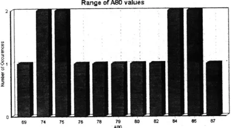
Figure 5.5 and 5.6 below show the rest of the output. A list of summary statistics is presented
that characterizes the output of the simulation in terms of the 80% Confidence (20& percentile) of the A80, the average A80, the mean A80, and a 95% confidence interval of the A80 availabilities.
A table displays the actual A80 availabilities output from the entire simulation as an A80 value
and frequency of occurrence, while the Graph is a histogram that displays this distribution of values from this table.
Figure 5.5: A80 Availability Results Output
A80 Statistics
80% Confidence of ABO values: 74.3
Average of ABO values: 79.85
50% Confidence of ABO values: 78.5 95% range of ABO values: 69 to 85
Range of ASO Results
S rr&%io Name AMO NntCrM Occurow"
WPEiEMO3 '69 1 WPTEMO 3 74 2 WPD2EMO 3 75 2 WPDEMO 3 76 1 WPDEMO-3 78 1 WPDEMO-3 79 1 WPDEM0-3 80 1 WFEIEMO-3 82 1 WPDEMO 84 2 WPDEMO-3 85 2 WPDEMO T ' 7 I
Figure 5.6: Availability Graph
Range of ASO values
69 74 75 78 78 79 8 82 84 85 87
When running a simulation in EMIT, the user can select before hand the type of output he or she would like to see by answering YES or NO to the Include Avail Table and Include Graph prompt boxes. By limiting the graphical output, time is saved in running and presenting simulation results.
6. Discussion
6.1 Interpretation of the Output
Since the output of the model is a distribution of A80 values, the interpretation thereof proves less than straightforward. Given the different ways to interpret the output from the simulation, several statistics are calculated and presented. These are:
1. 80% Confidence of A80
2. Average A80
3. Median A80
4. 95% Confidence Interval
Certainly it is helpful to know what A80 availability on average one could expect from the tool set. Therefore, one might look to the mean and/or median. Additionally, it is useful to discover to what degree we know that the average value represents the average of the population, so a 95% Confidence Interval of outcomes is presented. Furthermore, it is important to capture a measure of the dispersion of the output, and/or some measure of the predictability of the A80 output. A strong argument can be made that given an acceptance of the A80 statistic as a strong indicator of predictable and repeatable performance, the 20 percentile of the output A80 availabilities is a valuable representation of your tool group's predictable A80 performance - in essence, an
A80(A80).
Overall, it is important to realize that given the same system of equipment with the same PM schedules and same patterns of machine failures, a range of A80 performance can be expected, as demonstrated by the range of the model output. This information could be used to drive tool set improvement projects that focus first on reducing variation in the A80 availability, and then
raising the mean A80 of the machine group. The realization that A80 can vary will also color the interpretation of what it means to have a bad A80 week or month. Instead of viewing this
unusually low availability performance as having a special cause, you might realize that the system as designed is capable of producing such a low availability outcome, due to the random nature of the failure modes. This will have impacts on reactions and corrective actions to these types of situations.
6.2 Why 80% Confidence
The reasons that the 80% Confidence level (20th percentile) is used are the following (adapted
from the 80% Confidence Student Guide, Babikian et al):
1. Tool availability distributions vary from normal to non-normal distributions, and generally for
normal distributions one might look at standard deviations as a measure of predictability. In particular, one could choose 1 sigma on each side of the mean, giving us a lower confidence level of 16%. For non-normal distributions, one might choose the inner quartile range, or the
250 - 75* percentiles, leaving the lower confidence level of 75%. For practical purposes, the
generally used confidence level is chosen in between the two at 80%.
2. The Pareto Principle, which forwards that 80% of results are achieved by solving 20% of the problems, implies that the 80% confidence level is a good indicator for focusing tool
availability improvement.
3. Plotting Average Daily Availability of a tool set on a cumulative percentile graph shows that
in general the lowest performing days are outliers, and indicate days when special cause problems, or serious process excursions, have occurred. Since these are not common cause problems, and there is a mechanism already established to deal with these types of problems,