HAL Id: hal-00329411
https://hal.archives-ouvertes.fr/hal-00329411
Submitted on 22 Dec 2004
HAL is a multi-disciplinary open access
archive for the deposit and dissemination of
sci-entific research documents, whether they are
pub-lished or not. The documents may come from
teaching and research institutions in France or
abroad, or from public or private research centers.
L’archive ouverte pluridisciplinaire HAL, est
destinée au dépôt et à la diffusion de documents
scientifiques de niveau recherche, publiés ou non,
émanant des établissements d’enseignement et de
recherche français ou étrangers, des laboratoires
publics ou privés.
Distributed under a Creative Commons Attribution - NonCommercial| 4.0 International
License
Variations of the ionospheric electron density during the
Bhuj seismic event
A. Trigunait, Michel Parrot, S. Pulinets, F. Li
To cite this version:
A. Trigunait, Michel Parrot, S. Pulinets, F. Li. Variations of the ionospheric electron density during
the Bhuj seismic event. Annales Geophysicae, European Geosciences Union, 2004, 22 (12),
pp.4123-4131. �10.5194/angeo-22-4123-2004�. �hal-00329411�
SRef-ID: 1432-0576/ag/2004-22-4123 © European Geosciences Union 2004
Annales
Geophysicae
Variations of the ionospheric electron density during the Bhuj
seismic event
A. Trigunait1, M. Parrot1, S. Pulinets2, and F. Li1
1Laboratoire de Physique et Chimie de l’Environnement, Centre National de la Recherche Scientifique, Orl´eans, France 2Instituto de Geof´ısica, UNAM, Ciudad Universitaria, Delegaci´on de Coyoac´an, 04510, M´exico D.F., Mexico
Received: 4 February 2004 – Revised: 4 August 2004 – Accepted: 5 October 2004 – Published: 22 December 2004
Abstract. Ionospheric perturbations by natural geophysical
activity, such as volcanic eruptions and earthquakes, have been studied since the great Alaskan earthquake in 1964. Measurements made from the ground show a variation of the critical frequency of the ionosphere layers before and after the shock. In this paper, we present an experimen-tal investigation of the electron density variations around the time of the Bhuj earthquake in Gujarat, India. Sev-eral experiments have been used to survey the ionosphere. Measurements of fluctuations in the integrated electron den-sity or TEC (Total Electron Content) between three satellites (TOPEX-POSEIDON, SPOT2, SPOT4) and the ground have been done using the DORIS beacons. TEC has been also evaluated from a ground-based station using GPS satellites, and finally, ionospheric data from a classical ionospheric sounder located close to the earthquake epicenter are utilized. Anomalous electron density variations are detected both in day and night times before the quake. The generation mech-anism of these perturbations is explained by a modification of the electric field in the global electric circuit induced during the earthquake preparation.
Key words. Ionosphere (ionospheric disturbances) – Radio
Science (ionospheric physics) – History of geophysics (seis-mology)
1 Introduction
Since the great Alaskan earthquake in 1964 (Leonard and Barnes, 1965), many evidences of ionospheric perturbations after strong earthquakes have been reported (see, for exam-ple, the review by Blanc, 1985). The perturbations occur just after the shock and are due to acoustic waves which are amplified through the atmosphere because of the decreasing atmospheric density with increasing height.
Correspondence to: M. Parrot
(mparrot@cnrs-orleans.fr)
Furthermore, it has been shown that electric and mag-netic modifications could occur between a few hours and a few days before earthquakes in the seismic zone. Iono-spheric perturbations have also been observed a few days be-fore above the seismic zone. However, it must be noted that not all earthquakes produce such phenomena. Experiments close to some earthquakes have not recorded perturbations. This is a common factor of all precursors due to the com-plex nature of earthquakes. Some examples of these iono-spheric perturbations can be found in Sobolev and Husamid-dinov (1985), Fatkullin et al. (1989) and in the monographs edited by Hayakawa and Fujinawa (1994), and Hayakawa and Molchanov (2002). Such ionospheric anomalies are bet-ter detected during the night when the ionosphere is calm (see the review by Parrot et al., 1993). Increases as well as decreases of the critical frequencies are observed in the D-, E- and F-regions before earthquakes. Although this phenom-ena is not well understood, it could be related to a redistri-bution of the electric charges at the surface of the Earth and then in the Earth’s atmospheric system. Other hypotheses concerning the mechanism of these perturbations are given in Parrot et al. (1993), Molchanov (1993), Parrot (1995), and Pulinets et al. (2003). Ionospheric effects of aerosols and metallic ions emitted in the atmosphere above seismic regions are considered in Pulinets et al. (1994, 1997, and 1999). Pulinets et al. (2000) calculated the electric field gen-eration on the Earth’s surface and in the atmosphere. It was shown that the additional flux of metallic aerosols leads to the strengthening of an anomalous electric field. This elec-tric field (in local region inside atmospheric layers) was eval-uated. It was found that the night-time field penetration effi-ciency is larger than during the daytime and that it depends upon the size of the vertical field Ezlocalization layer. Pu-linets et al. (2002) introduces the concept of atmospheric plasma appearing in the near ground layer of the atmosphere under the action of radon radioactivity in seismically ac-tive regions. Such plasma could trigger or perturb different kinds of EM emissions at various frequencies observed ex-perimentally before strong earthquakes. The paper focuses
4124 A. Trigunait et al.: Variations of the ionospheric electron density
on the seismogenic variations on the higher altitude-upper ionosphere and magnetosphere-small- and large-scale irreg-ularities within F-layers of ionosphere and magnetospheric duct formation.
Pulinets and Legen’ka (2002) revealed a strong modifi-cation of the equatorial anomaly structure prior to strong earthquakes by the analysis of topside ionograms obtained on board Intercosmos-19 satellite. Equatorial anomaly (EA) may increase (deepen) or attenuate (be filled up), depending upon the local time. The most important parameter indicat-ing that EA is modified prior to earthquake is theB2u param-eter. B2u is the half thickness of the topside part of the Ne(h) profile of the F2-layer. The EA modification results on the basis of satellite data are confirmed by the data of ground-based observations.
Pulinets and Legen’ka (2003) have shown that seismic ionospheric disturbances are strongly time dependent before the beginning of the main shock. Seismic ionosphere dis-turbances are generated weekly, several days before the first shock, but at that moment the displaced region is not located above the epicentre, but rather displaced from it. These dis-turbances can be transferred along magnetic field lines into the conjugate regions in the opposite hemisphere. Three earthquakes of different latitudes (High latitude, Alaska; Mid latitude, Central Italy; and Low latitude, New Zealand) have been considered. Moreover, data of vertical sounding of the ionosphere performed by the Alouette-1 and Intercosmos-19 satellites have been taken, along with the data of vertical sounding of the ionosphere by ground-based instruments.
Variations of the critical frequencies of the ionospheric layers were mainly observed with ground-based ionospheric sounders, but measurements of Total Electron Content (TEC) by satellites can also be used (Evans, 1977). The TEC gives the sum of the electron density between the altitude of the satellite and the ground. Therefore, this parameter is mainly related to the density in the F-layer which is larger than in the others. Calais and Minster (1995) have used this method to detect perturbations due to an earthquake. A statistical study with the TEC data from TOPEX-POSEIDON has been performed by Zaslavski et al. (1998) to check correlations between ionospheric perturbations and seismic activity. This work is similar to the work of Liu et al. (2002), who used a method to derive the ionospheric TEC from data recorded by a network of the Global Positioning Systems (GPS) in Taiwan. Based on the network data the latitude time-TEC (LTT) plots are constructed and showed that 1–4 days prior to three earthquake onsets, TEC values decrease and anomaly crests move towards the equator. Further, the simultaneously deduced overhead TEC and the foF2 observed at Chung-Li during the three earthquakes are compared and examined. The recent publication of Liu et al. (2004), where a statis-tical analysis of TEC anomalies has been performed before strong earthquakes (M>6) at Taiwan, claims a leading time of 5 days before the seismic shock for the ionospheric pre-cursors.
All these concerns about the ionospheric anomalies have been compiled in a review paper by Pulinets et al. (2003).
Thus the aim of this paper is to study the ionosphere and as-sociated parameters recorded by various experiments above the Gujarat active seismic zone around the time of the Bhuj earthquake. A workshop report about this event can be found in Singh and Ouzounov (2003). The experimental equip-ments and the data selection are described in Sect. 2, whereas the results are presented in Sect. 3. Discussions and conclu-sions are given in Sect. 4.
2 The data
2.1 The Bhuj earthquake
The Bhuj earthquake shook the Indian province of Gujarat on the morning of 26 January 2001 at 03:16 GMT (08:46 LT). This devastating earthquake had a magnitude Ms=7.6, and a
depth of approximately 24 km. The exact location of the epi-center was 23.4◦N, 70.32◦E, approximately at 20 km from Bhuj (population 150 000). Since this earthquake occurred in a heavily industrialised region of India, it caused a lot of casualties. Numerous aftershocks exceeding Ms=5 have been
reported and one aftershock had a magnitude Ms=5.9. It took
place on 28 January 2001 at 06:32 IST. Up until 31 January 2001 hundred aftershocks with magnitudes ranging between 2.8 and 5.9 have occurred. The more important ones are dis-played in the bottom panel of Fig. 4.
2.2 The TEC data from TOPEX-POSEIDON
We used the data of the TOPEX/POSEIDON satellite which is dedicated to space oceanography and has two altimetric systems for measuring the altitude of the satellite above the sea surface. Measurement of fluctuations in the integrated electron density or TEC (Total Electron Content) between the satellite and the ground is used to remove the ionospheric influences in order to obtain a better estimation of the alti-tude (Monaldo, 1993). Typical examples of TEC variations are shown, for example, in Robinson and Beard (1995), and Zlotnicki (1994).
The TOPEX-POSEIDON satellite carries a dual frequency altimeter operating at frequencies of 13.6 GHz (Ku-band) and 5.2 GHz (C-band). The data from the dual frequency altimeter are obtained with a good time resolution (1 s) but unfortunately they are not valid above land. So, in this study we have used the data from the DORIS system (Fleury et al., 1991; Escudier et al., 1993) which is valid everywhere. However, the amplitude resolution is low because the DORIS system uses a set of ground-based stations (∼50) located at the surface of the Earth to determine the vertical sub-satellite values.
Our data are from the AVISO CD-Roms (AVISO, 1992). We used the ionospheric correction for the altitude measure-ment which is expressed in millimetres. This quantity is di-rectly proportional to TEC. The time resolution of the data is one point by second. At Ku-band, this parameter can reach up to −250 mm during high solar activity. It must be noticed that this negative value, in fact, corresponds to a positive
Fig. 1. Orbit tracks of the satellite TOPEX-POSEIDON around the position of the Bhuj earthquake (see also Table 1).
increase of electron density. In the AVISO CD-Roms, ex-pected ionospheric corrections from the Bent model are also given. The altitude of the TOPEX-POSEIDON satellite is 1340 km and it covers the geographic range from 66◦N to 66◦S. A particularity of this satellite is that its ground tracks are always identical, but it is not a Sun-synchronous satel-lite. Therefore, a study of parameter variations versus the local time can be performed at a given place. The satellite re-turns every 10 days at the same location, and at the equator, the distance between 2 ground tracks is ∼300 km, whereas the distance between 2 consecutive orbits is ∼3000 km. The data have been studied during one month around the earth-quake time. Figure 1 presents the ground tracks of the satel-lite TOPEX-POSEIDON around the Bhuj location. In the middle, the star indicates the position of the epicentre. The satellite regularly returns on the same tracks which have been labelled A, B, C, and D. Tracks A and C are upgoing tracks, whereas B and D are downgoing tracks. The days and aver-age hours in UT (LT=UT+5.5 h) of each passes are given in the Table 1. It must be noted that tracks A and C correspond to daytime (the ionospheric correction is higher because the TEC is much important) whereas tracks B and D correspond to nighttime. Two months of data centred on the time of the earthquake have been considered.
2.3 The TEC data from the satellites SPOT2 and SPOT4 SPOT2 and SPOT4 are two satellites devoted to the Earth’s observation. The altitude of these satellites is ∼810 km and their orbit inclination is 98◦. They have both a DORIS sys-tem similar to the one on board TOPEX-POSEIDON which was presented in the above section. However, the presenta-tion of the ionospheric data is different in such a sense that
Table 1. Days and hours corresponding to the TOPEX-POSEIDON
passes along the tracks A, B, C, and D of Fig. 1. Day Hour (UT) Track 01 Jan 13.45 A 04 Jan 13.00 C 05 Jan 23.25 B 08 Jan 22.35 D 11 Jan 11.45 A 15 Jan 21.20 B 21 Jan 09.45 A 24 Jan 09.00 C 25 Jan 19.20 B 28 Jan 18.30 D 31 Jan 07.45 A 03 Feb 07.00 C 04 Feb 17.20 B 07 Feb 16.30 D 10 Feb 05.40 A 13 Feb 04.55 C 14 Feb 15.15 B 17 Feb 14.30 D 20 Feb 03.40 A 23 Feb 02.50 C 24 Feb 13.15 B 27 Feb 12.30 D
slant TEC values between satellites and ground-based sta-tions are given. The available parameter is an ionospheric correction in m/s given by
I ono = −ac
dt
[k2CET2ver−k1CET1ver]
4126 A. Trigunait et al.: Variations of the ionospheric electron density
Fig. 2. Positions of the SPOT2 subionospheric points around three different DORIS stations during 24 January passes.
where a is a constant (40.22/c in m2/(electron.s)), c is the light velocity, dt is the counting period, CET 1ver and
CET2ver are the vertical TEC at the beginning and at the end of the counting period, respectively, and F is the emis-sion frequency. The geometric factor k of correction is given by
k(r, E) =p r
r2−(R
Tcos E)2
, (2)
where r is the position radius of the subionospheric point (r=RT+hm+50 km), RT is the Earth radius, hm is the subionospheric altitude (altitude of the maximum of elec-tron density) , and E is the elevation angle of the satellite relatively to the station. As a slant TEC estimation is done, the subionospheric point is the point at an altitude equal to 350 km which belongs to the line between the satellite and the ground-based DORIS station. It gives the best position of the TEC estimation because 350 km is the average altitude of the maximum of the electron density. Therefore, the pa-rameter Iono given by Eq. (1) is more related to a TEC time variation than to the TEC parameter itself.
Figure 2 represents the positions of these subionospheric points for each passes of the satellite SPOT2 close to the DORIS stations which are around the epicenter of the Bhuj earthquake on 24 January 2001. Using Eq. (1) with the method described in Fleury et al. (1991), the TEC parameters have been estimated for each satellite passes. This method only assumes a latitudinal variation of TEC.
2.4 The TEC data from the Bangalore ground-based station We use data from a ground-based station located at Banga-lore (Lat. 13.021, Long. 77.57). This GPS station, named
IISC, belongs to the NASA Flinn global network for contin-uous GPS analysis. Bangalore is quite far from the epicenter (1400 km), but it falls in the area of this earthquake prepa-ration which depends on the magnitude (Dobrovolsky et al., 1979).
2.5 The ionospheric data from the Ahemadabad ground-based sounder station
We used the data of Ahemadabad ionospheric station (23.02◦N, 72.6◦E) located at 220 km from Bhuj. Data has been collected from the SPIDR (Space Physics Interactive Data Resource) NOAA Satellite and Information Services (http://spidr.ngdc.noaa.gov/). The maximum time resolution of these data is 1 h. Two parameters which characterise the F2ionospheric layer have been taken into account: the
char-acteristic frequency foF2 and the virtual height hpF2.
3 The results
Figure 3a shows the variations of the TOPEX-POSEIDON ionospheric data recorded along the tracks A and C (see Table 1) as a function of the latitude. It corresponds to data recorded in the daytime but not at the same hours, because there is a time shift due to satellite passes. It is shown that the ionospheric correction increases for days which are close to 26 January, the earthquake’s day, and decreases as far as we move away from this date. On 24 January, around 09:00 UT (14:30 LT), the ionospheric correction is much more impor-tant. Although all these data are recorded in local daytime (see Table 1), this tendency could be attributed to a normal time variation because TEC values are usually maximum just after noon in local time. Then a comparison has been done
(a)
(b)
Fig. 3. Daytime variations observed by TOPEX-POSEIDON, (a)
values of the ionospheric corrections as function of the latitude (see also Table 1), (b) differences between the ionospheric corrections and the Bent model as a function of the latitude.
with a model, and the corresponding differences with the Bent ionospheric model are plotted in Fig. 3b. Looking for differences with an absolute value larger than 20 mm, it is again observed that largest variations occur for days close to the earthquake’s day, except on 13 February. Although it is a date far from the earthquake’s day, the data recorded on 13 February depict a large difference with the ionospheric model. This can be explained by the magnetic activity which reaches during this day its maximum value over the time interval of two months, as it is shown in the last panel of Fig. 10.
The results from SPOT2 and SPOT4 are given in Fig. 4. We have only considered the data from the KITB station which is closest to the epicentre (see Fig. 2). The top panel of Fig. 4 shows the variation of the ionospheric correction given by Eq. (1) for the two satellites passes during an inter-val of two months around the time of the Bhuj earthquake. The passes occurred between 11:00 and 13:00 LT, and for
Fig. 4. Top panel: TEC variations in time as a function of the
lat-itude for the two satellites SPOT2 and SPOT4 during two months around the time of the Bhuj earthquake. It concerns the data from the KITB station (see Fig. 2). Middle panel: Corresponding TEC values in TEC units (1016m−2). Bottom panel: Magnitude and occurrence of the main aftershocks. In the two first panels the hori-zontal full line represents the mean value, whereas the dashed lines indicate the variance, and the vertical line indicates the time of the Bhuj earthquake.
each pass the data have been averaged for latitudes between 25◦and 33◦, in order to obtain a single measurement per day. The horizontal full line indicates the mean value over the two months and the dashed lines indicate the variance. It is ob-served that an important TEC time variation occurred on 24 January. It corresponds to a SPOT2 pass which is in red, in Fig. 2.
Around the time of the Bhuj earthquake, another impor-tant TEC variation has been recorded on 29 January. This last anomalous variation can be attributed to aftershock ac-tivity, as it can be observed on the bottom panel of Fig. 4. Other important TEC variations have been recorded at the end of February which can be imputed to our long time in-terval of observations. Two factors can be involved: i) a time shift of the observations which took place around 11:00 LT at the beginning of January and around 13:00 LT at the end of February (this last local time corresponds, on average, to a maximum of TEC), and ii) a seasonal variation (Codrescu et al., 1999). The middle panel of Fig. 4 represents the TEC pa-rameters obtained by the method mentioned in Sect. 2.3. As in the top panel, the TEC values correspond to registrations between 11:00 and 13:00 LT, and they are averaged for lati-tudes between 25◦and 33◦. A maximum value is observed on 20 January, six days before the earthquake. Explanations concerning other values exceeding the variance at the end of February are similar to the ones given for the top panel.
Figure 5 represents the TEC data recorded at Bangalore station from 16 January until 30 January. In this time inter-val, two anomalous variations appear on 21 and 25 January in the afternoon – evening sector.
4128 A. Trigunait et al.: Variations of the ionospheric electron density
Fig. 5. Variations of the TEC data recorded by the Bangalore station
during the second half of January 2001.
16 17 18 19 20 21 22 23 24 25 26 January, 2001 -60 -40 -20 0 20 40 60 δ fo F2 ( % )
Fig. 6. Critical frequency deviation of the Ahemadabad station data
from 16 to 26 January 2001.
It was shown (Pulinets, 1998) that a few days before the strong earthquakes the ionosphere variability increases. The variability of the ionosphere can be estimated by different ways (Forbes et al., 2000; Rishbeth and Mendillo, 2001) but the most appropriate and accepted is the value of the critical frequency deviation from the monthly median:
δf oF2(%) = 100(f oF 2 − f oF 2)/f oF 2 , (3)
where foF2 is the critical frequency, and f oF 2 is the monthly median. Statistical analysis shows that a 25% threshold is an indicator of the “normal” state of the iono-sphere. Figure 7, for critical frequency deviations before the time of Bhuj earthquake, demonstrates the increase of the variability starting from 21 January (5 days before the seis-mic shock).
In Liu et al. (2004), a statistical process was devel-oped to reveal possible ionospheric precursors: the inter-quartile range IQR is calculated to construct the upper bound
˜
X+I QRand lower bound ˜X−I QRfor the data estimation
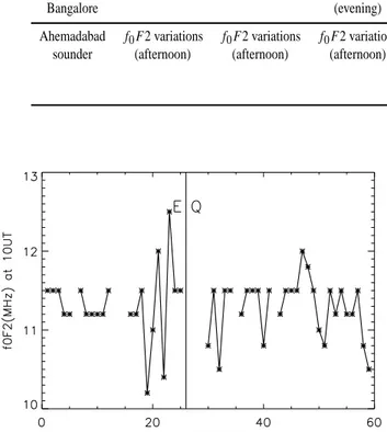
Fig. 7. foF2 variations on 23 January 2001 in a continuous line with
points. In the green line, it is the monthly median, in the red dashed line it is the upper bound f oF 2+2σ , and in the blue dashed line it is the lower bound f oF 2−2σ .
where ˜Xis the 15-day running mean. Here instead of ˜Xwe use the monthly median. Liu et al. (2004) estimated IQR as 1.34σ , where σ is the standard deviation. To make the condi-tion more rigorous we took in our processing a 2σ threshold. Figure 8 shows the results of the processing for 23 January. The black line with points represents the real measurements of the critical frequency, the green line represent the monthly median, and the dashed red and blue lines represents the up-per and lower bounds of f oF 2+2σ and f oF 2−2σ , respec-tively. One can clearly see from the figure that the value at 10:00 UT is out of the 2σ upper bound, and that at 17:00 and 18:00 UT the value is out of the 2σ lower bound. They both show anomalous deviations of the critical frequency. To demonstrate this anomalous behavior we bring the data for the variations of the critical frequency at 10:00 UT in Fig. 8. For the month of January 2001 the value of the critical fre-quency at 10:00 UT is within the range between 11.0 and 11.5 MHz, and only a few days before the seismic shock one can see the sharp drop and then gradual increase of the criti-cal frequency. This behavior is completely different in com-parison with the whole month’s behavior. As the epicenter was close to the station, it must be noted that a large gap is observed just after the quake. In February, fewer variations are observed that can be attributed to the aftershock activity (see the bottom panel of Fig. 4).
All critical ionospheric frequencies foF2 recorded by the Ahemadabad station during January and February 2001 are shown in Fig. 9. It represents the hourly variations of
foF2 as a function of the days, which are color-coded
ac-cording to the scale on the right. The missing data have been forced to zero values. An interesting information is contained in the station records: at 20:00 UT on 25 Jan-uary, there is no foF2 and hpF2 data due to the presence
of a spread-F-layer. Otherwise, nothing is unusual to re-port from Fig. 9, except an increase in the 16:00–18:00 UT time interval (21:30–23:30 LT) which stops 3 days before the
Table 2. Main ionospheric variations observed by various experiments before the Bhuj event.
January days 19 20 21 22 23 24 25 26
TOPEX TEC decrease
(daytime)
SPOT TEC increase TEC variations
(daytime) (daytime)
TEC TEC decrease TEC decrease
Bangalore (evening) (evening)
Ahemadabad f0F2 variations f0F2 variations f0F2 variations f0F2 variations f0F2 variations Spread F sounder (afternoon) (afternoon) (afternoon) (afternoon) (afternoon) (night)
hpF2 increase
(night)
Fig. 8. Critical frequency variations at 10:00 UT for January and
February 2001 at Ahmadabad ionospheric station.
quake. This anomalous increase has an important effect on the monthly average value, as can be seen on Fig. 7.
Particular attention has been given to the nighttime and we have checked the variation of hpF2 during the January
and February months of several years. The results are pre-sented in Fig. 10. The top panel shows the averaged values of hpF2which take into account the measurements at 22:00,
23:00 and 24:00 UT (03:30, 04:30, 05:30 LT). This parameter is plotted as a function of the days for January and February 1998. The thick dashed line represents the averaged values of this parameter over the two months, whereas the two thin dashed lines are related to the standard deviation σ . The sec-ond panel represents the variation of the magnetic activity in-dex Apas a function of the same days. The two middle pan-els concerns the same parameters for the year 1999 whereas the two bottom panels are related to 2001, the year of the event (no ionospheric data are available for the year 2000). It is interesting to compare the variations of hpF2with Ap for these three years. In 1998, during the two months January
Fig. 9. Hourly variations of foF2 in UT at the Ahemadabad
iono-spheric station during January and February 2001. The data are color-coded according to the scale on the right.
and February, the Apindex does not exceed 40 and hpF2
re-mains between +σ and −σ . In 1999, the Apindex is equal to 40 and more on 13 January and 19 February and this induces at the same time a large increase in hpF2. In 2001, Ap is much less than 40 during the 2 months and then a large vari-ation of hpF2 is not expected. However, three days before
the quake we observe an increase larger than 2σ . Another increase on 31 January could be related to aftershocks.
4 Discussion and conclusions
Table 2 sums up the ionospheric observations done before the Bhuj earthquake. The following anomalous ionospheric variations have been observed:
– The TEC from TOPEX indicates a decrease on 21
4130 A. Trigunait et al.: Variations of the ionospheric electron density
Fig. 10. Variations of an average hpF2 value taken between 22:00, 23:00, and 24:00 UT at the Ahemadabad ionospheric station and variations
of the magnetic index Apas a function of the January and February days. From the top to the bottom, the plots are done for the year 1998,
1999, and 2001 (the quake occurred on 26 January 2001).
– The TEC from SPOT2 and SPOT4 indicates an increase
on 20 January (daytime) and a perturbation on 24 Jan-uary around 06:30 UT (this is confirmed by the sounder because the data corresponding to this time are not available).
– The TEC from the Bangalore station shows similar
af-ternoon – evening perturbations (decrease) on 21 and 25 January.
– The ionospheric sounder close to the epicenter
indi-cates an increase of the foF2 variability during the night of 21 January. An anomalous behaviour of foF2 at 10:00 UT is shown several days before the quake. An increase in foF2 is observed several days before the quake during evening time (21:30–23:30 LT). An in-crease of hpF2is observed 3 days before the quake
dur-ing nighttime (03:30, 04:30, 05:30 LT). On 25 January around 20:00 UT, the ground-based sounder detects a spread-F-layer at this local nighttime.
From the observations, we can conclude that the iono-sphere behavior changes a few days before the seismic shock with increased variability starting on 19 January, which can be interpreted as anomalous pre-seismic ionospheric varia-tions.
It is common knowledge that the ionosphere is mainly un-der the control of the solar activity and that it can be affected
by TIDs (Traveling Ionospheric Disturbances). However, we have shown anomalous behaviours prior to the Bhuj earth-quake relative to a large time interval around the event time. All these anomalous perturbations depend on the time and the latitude of the observations. This is in agreement with previous events reported by Pulinets and Legen’ka (2002, 2003) and Liu et al. (2001, 2002).
A hypothesis to explain these ionospheric perturbations is related to the action of the electric field. Due to the stress of the rocks, electric charges could appear at the Earth’s surface and change currents in the atmosphere – ionosphere system. The effects of these electric fields on the ionosphere were modelled in Pulinets et al. (2000). It is noteworthy that, in relation to the possible mechanisms described in Sect. 1, Virk et al. (2003) have observed a radon anomaly on 22 January 2001.
Acknowledgements. Two authors wish to acknowledge the financial
support from IFCPAR (Indo-French Centre for the Promotion of Advanced Research or CEFIPRA – Centre Franco-Indien pour la promotion de la Recherche Avanc´ee) under the Research Project 2807-1. We are thankful to J.-J. Valette (CLS) for his help to get the ionospheric DORIS data.
Topical Editor M. Lester thanks two referees for their help in evaluating this paper.
References
AVISO, User Handbook: Merged TOPEX POSEIDON products, Rep. AVI-NT-02-101-CN, 2nd Ed., CNES, Toulouse, France, 1992.
Blanc, E.: Observations in the upper atmosphere of infrasonic waves from natural or artificial sources: A summary, Ann. Geo-phys., 3, 673–679, 1985.
Calais, E. and Minster, J. B.: GPS detection of ionospheric pertur-bations following the January 17, 1994, Northridge earthquake, Geophys. Res. Lett., 22, 1045–1048, 1995.
Codrescu, M. V., Palo, S. E., Zhang, X., Fuller-Rowell, T. J., and Poppe, C.: TEC climatology derived from TOPEX/POSEIDON measurements, J. Atmos. Sol. Terr. Phys., 61, 281–298, 1999. Dobrovolsky, I. R., Zubkov, S. I., and Myachkin, V. I.:
Estima-tion of the size of earthquake preparaEstima-tion zones, Pageoph., 117, 1025–1044, 1979.
Escudier, P., Picot, N., and Zanife, O. Z.: Altimetric ionospheric correction using DORIS Doppler data in Environmental Effects on Spacecraft Positioning and Trajectories, Geophys. Monogr., 73, IUGG, 13, 61–71, 1993.
Evans, J. V.: Satellite beacon contributions to studies of the struc-ture of the ionosphere, Rev. Geophys. Space Phys., 15, 325–350, 1977.
Fatkullin, M. N., Zelenova, T. I., and Legenka, A. D.: On the ionospheric effects of asthenospheric earthquakes, Phys. Earth Planet. Inter., 57, 82–87, 1989.
Fleury, R., Foucher, F., and Lassudrie-Duchesne, P.: Global TEC measurement capabilities of the Doris system, Adv. Space Res., 11 (10), 51–54, 1991.
Forbes, J. M., Palo, S. E., Zhang, X. L.: Variability of the iono-sphere, J. Atm. Sol. Terr. Phys., 62, 685–693, 2000.
Hayakawa, M. and Fujinawa, Y. (Eds): Electromagnetic Phenom-ena Related to Earthquake Prediction, Terra Scientific Publishing Company, Tokyo, Terrapub, 1994.
Hayakawa, M. and Molchanov, O. A. (Eds): Seismo Electromag-netics: Lithosphere-Atmosphere-Ionosphere coupling, Terra Sci-entific Publishing Company, Tokyo, Terrapub, 2002.
Leonard, R. S. and Barnes Jr., R. A.: Observations of ionospheric disturbances following the Alaska earthquake, J. Geophys. Res., 70, 1250–1253, 1965.
Liu, J. Y., Chen, Y. I., Chuo, Y. J., and Tsai, H. F.: Variations of ionospheric total electron content during the Chi-Chi earthquake, Geophys. Res. Lett., 28 (7), 1383–1386, 2001.
Liu, J. Y., Chuo, Y. J., Pulinets, S. A., and Tsai, H. F.: A study on the TEC perturbations prior to the Rei-Li, Chi-Chi, and Chia-Yi earthquakes, in: Seismo Electromagnetics: Lithosphere-Atmosphere-Ionosphere Coupling, edited by: Hayakawa, M. and Molchanov, O. A., Terrapub, Tokyo, 297–301, 2002.
Liu, J. Y., Chuo, Y. J., Shan, S. J., Tsai, Y. B., Pulinets, S. A., and Yu, S. B.: Pre-earthquake ionospheric anomalies monitored by GPS TEC, Ann. Geophys., 22, 1585–1593, 2004.
Molchanov, O. A.: Wave and plasma phenomena inside the iono-sphere and magnetoiono-sphere associated with earthquakes, in: Re-view of Radio Science 1990–1992, edited by: Ross Stone, W., Oxford University Press, Oxford, 591–600, 1993.
Monaldo, F.: TOPEX ionospheric height correction precision esti-mated from prelaunch test results, IEEE Trans. Geosci. Remote Sensing, 31, 371–375, 1993.
Parrot, M., Achache, J., Berthelier, J. J., Blanc, E., Deschamps, A., Lefeuvre, F., Menvielle, M., Plantet, J. L., Tarits, P., and Vil-lain, J. P.: High-frequency seismo-electromagnetic effects, Phys.
Earth Planet. Inter., 77, 65–83, 1993.
Parrot, M.: Electromagnetic noise due to earthquakes in Handbook of Atmospheric Electrodynamics, Vol. II, edited by: Volland, H., CRC Press, Boca Raton, 95–116, 1995.
Pulinets, S. A., Legen’ka, A. D., and Alekseev, V. A.: Pre-earthquake ionospheric effects and their possible mechanisms, in: Dusty and Dirty Plasmas, Noise, and Chaos in Space and in the Laboratory, edited by: Kikuchi, H., Plenum Press, New York, 545–557, 1994.
Pulinets, S. A., Alekseev, V. A., Legen’ka, A. D., and Khegai, V. V.: Radon and metallic aerosols emanation before strong earth-quakes and their role in atmosphere and ionosphere modification, Adv. Space Res., 20, N11, 2173–2176, 1997.
Pulinets, S. A.: Seismic activity as a source of ionospheric variabil-ity, Adv. Space Res., 22, 903–906, 1998.
Pulinets, S. A., Alekseev, V. A., Boarchuk, K. A., Hegai, V. V., Depuev, V. K.: Radon and ionosphere monitoring as a means for strong earthquakes forecast, Il Nuovo Cimento, 22C, N3-4, 621–626, 1999.
Pulinets, S. A., Boyarchuk, K. A., Hegai, V. V., Kim, V. P., and Lomonosov, A. M.: Quasielectrostatic model of atmosphere-thermosphere-ionosphere coupling, Adv. Space Res., 26 (8), 1209–1218, 2000.
Pulinets, S. A., Boyarchuk, K. A., Hegai, V. V., and Kare-lin, A. V.: Conception and model of seismo-ionosphere-magnetosphere coupling, in: Seismo Electromagnetics: Lithosphere-Atmosphere-Ionosphere Coupling, edited by: Hayakawa, M. and Molchanov, O. A., Terrapub, Tokyo, 353–361, 2002.
Pulinets, S. A. and Legen’ka, A. D.: Dynamics of the near-equatorial ionosphere prior to strong earthquakes, Geomag-netism and Aeronomy, 42 (2), 227–232, 2002.
Pulinets, S. A. and Legen’ka, A. D.: Spatial-temporal characteris-tics of large scale disturbances of electron density observed in the ionospheric F-region before strong earthquakes, Cosmic Re-search, 41 (3), 221–229, 2003.
Pulinets, S. A., Legen’ka, A. D., Gaivoronskaya, T. V., and Depuev, V. K.: Main phenomenological features of ionospheric precur-sors of strong earthquakes, J. Atm. Sol. Terr. Phys., 65(16–18), 1337–1347, 2003.
Rishbeth, H. and Mendillo, M.: Patterns of ionospheric variability, J. Atm. Sol.-Ter. Phys., 63, 1661–1680, 2001.
Robinson, T. R. and Beard, R.: A comparison between electron con-tent deduced from the IRI and that measured by the TOPEX dual frequency altimeter, Adv. Space Res., 16 (1), 155–158, 1995. Singh, R. P. and Ouzounov, D.: Earth processes in wake of Gujarat
earthquake reviewed from space, EOS, 84 (26), 244, 2003. Sobolev, G. A. and Husamiddinov, S. S.: Pulsed
electromag-netic earth and ionosphere field disturbances accompaying strong earthquakes, Earthquake Prediction Res., 3, 33–41, 1985. Virk, H. S., Vivek Valia, Bajwa, B. S., and Kumar, P.: Radon
precur-sory signals of Chamoli and Bhuj earthquakes, abstract in: Inter-national Workshop on Earth System Processes related to Gujarat Earthquake Using Space Technology, Kanpur, India, 27–29 Jan-uary, 2003.
Zaslavski, Y., Parrot, M., and Blanc, E.: Analysis of TEC measure-ments above active seismic regions, Phys. Earth Plan. Inter., 105, 219–228, 1998.
Zlotnicki, V.: Correlated environmental corrections in TOPEX/POSEIDON, with a note on ionospheric accuracy, J. Geophys. Res., 99, 24 907–24 914, 1994.