HAL Id: hal-00317270
https://hal.archives-ouvertes.fr/hal-00317270
Submitted on 19 Mar 2004
HAL is a multi-disciplinary open access
archive for the deposit and dissemination of
sci-entific research documents, whether they are
pub-lished or not. The documents may come from
teaching and research institutions in France or
abroad, or from public or private research centers.
L’archive ouverte pluridisciplinaire HAL, est
destinée au dépôt et à la diffusion de documents
scientifiques de niveau recherche, publiés ou non,
émanant des établissements d’enseignement et de
recherche français ou étrangers, des laboratoires
publics ou privés.
irregularities over Trivandrum
D. Tiwari, A. K. Patra, C. V. Devasia, R. Sridharan, N. Jyoti, K. S.
Viswanathan, K. S. V. Subbarao
To cite this version:
D. Tiwari, A. K. Patra, C. V. Devasia, R. Sridharan, N. Jyoti, et al.. Radar Observations of 8.3-m
scale equatorial spread F irregularities over Trivandrum. Annales Geophysicae, European Geosciences
Union, 2004, 22 (3), pp.911-922. �hal-00317270�
© European Geosciences Union 2004
Geophysicae
Radar Observations of 8.3-m scale equatorial spread F irregularities
over Trivandrum
D. Tiwari1, A. K. Patra2, C. V. Devasia1, R. Sridharan1, N. Jyoti1, K. S. Viswanathan1, and K. S. V. Subbarao1 1Space Physics Laboratory, Vikram Sarabhai Space Center Trivandrum, 695022, India
2National MST Radar Facility, Tirupati, 517502, India
Received: 4 March 2003 – Revised: 2 September 2003 – Accepted: 8 October 2003 – Published: 19 March 2004
Abstract. In this paper, we present observations of
equa-torial spread F (ESF) irregularities made using a newly in-stalled 18 MHz radar located at Trivandrum. We character-ize the morphology and the spectral parameters of the 8.3-m ESF irregularities which are found to be remarkably differ-ent from that observed so extensively at the 3-m scale size. We also present statistical results of the irregularities in the form of percentage occurrence of the echoes and spectral parameters (SNR, Doppler velocity, Spectral width). The Doppler spectra are narrower, less structured and less vari-able in time as compared to those observed for 3-m scale size. We have never observed the ESF irregularity veloci-ties to be supersonic here unlike those at Jicamarca, and the velocities are found to be within ±200 ms−1. The spectral
widths are found to be less than 150 ms−1. Hence, the
veloc-ities and spectral width both are smaller than those reported for 3-m scale size. The velocities and spectral widths are fur-ther found to be much smaller than those of the American sector. These observations are compared with those reported elsewhere and discussed in the light of present understanding on the ESF irregularities at different wavelengths.
Key words. Ionoshphere (equatorial ionosphere, plasma
waves and instabilities; ionospheric irregularities)
1 Introduction
The plasma irregularities in the equatorial F-region manifest in the form of diffuse ionogram and are referred to as equa-torial spread F (ESF) (Berkner and Wells, 1934). ESF is now known to be a manifestation of ionospheric interchange-instabilities such as the Rayleigh-Taylor or the gradient-drift instability, responding to the steep density gradient in the nighttime equatorial F-region. The general understanding is that, in the linear regime of these instabilities, only the bot-tomside of the F-region becomes unstable and in the nonlin-Correspondence to: D. Tiwari
diwakartiwari@yahoo.com
ear regime, these instability related depletion channels pene-trate through the F-region peak electron density well into top-side. These channels are referred to as plasma bubbles and display plume-like structures in the radar backscatter map (e.g. Woodman and LaHoz, 1976). Due to high conductivity along the geomagnetic north-south direction, these structures are spread along the magnetic field lines and are observed at all latitudes within about ±20◦latitude (Dyson and Benson, 1978). The instability processes at work in the F-region gen-erate plasma density irregularities with scale sizes ranging from a few centimeters to hundreds of kilometers. These ir-regularities have been studied using coherent and incoherent scatter radars (e.g. Woodman and LaHoz, 1976; Tsunoda et al., 1979; Tsunoda, 1980; Towle, 1980; Hysell et al., 1994; Hysell and Woodman, 1997; Patra et al., 1997; Rao et al., 1997; Hysell and Burcham, 1998), radio beacons (e.g. Basu et al., 1988), rocket and satellite in situ instrumentation (e.g. McClure et al., 1977; Kelley et al., 1986; Hanson and Bamg-boye, 1984; Pfaff et al., 1997; Sinha et al., 1999) and airglow observations (e.g. Weber et al., 1978; Mendillo and Baum-gardner, 1982; Sinha et al., 2001), since they are sensitive to different parts of the scale-size spectrum of the irregularities. The early observations which motivated much of the theo-retical and simulation work were provided by the high power VHF and UHF backscatter radars at Jicamarca and Kwajalein (Farley et al., 1970; Woodman and LaHoz, 1976; Tsunoda et al., 1979; Tsunoda, 1980; Towle, 1980). In late nineties, these irregularities have also been studied over low latitudes and the ESF structures were found to be remarkably differ-ent in their morphology as compared to the equator (Hy-sell et al., 1994; Patra et al., 1997; Rao et al., 1997). The above radar observations relate directly to short-scale irreg-ularities of about 3 m, 1 m, 36 cm and 11 cm wavelengths. Most of the observations, however, correspond to a 3-m scale size of the irregularities. While observations correspond-ing to scale sizes less than 3 m have been known, very little is known about the scale sizes larger than 3 m. HF radars have been used to measure the F-layer drift (e.g. Jayachan-dran et al., 1987) but they have been done at a frequency
less than 5.5 MHz, much less than the maximum plasma fre-quency of the F-region. Such a frefre-quency is not adequate to study the ESF irregularities when the ESF is fully developed (depleted). ESF irregularities have been studied using the HF sounders (ionosonde), which display diffuse ionograms. This, however, gave only the occurrence statistics of ESF and some morphology of ESF in terms of range spread F and frequency spread F. Hence, finer details of the irregularities responsible for radio scattering are missing in the ionogram studies. It is also difficult to understand when ESF irreg-ularities are fully developed. HF radar studies well above the plasma frequency are very rare, except those done in the early years of ESF studies by Clemesha (1964) and Kelle-her and Skinner (1971). The observations made by Cleme-sha (1964) and Kelleher and Skinner (1971) correspond to a radar frequency of 18 MHz and 27.8 MHz, respectively. Since then, few observations have been made at these fre-quencies. Some spectral signatures were shown by Cleme-sha (1964) at 18 MHz but they are limited. Another study on ESF made using the HF sounder by Cecile et al. (1996) shows some signature of plasma density depletions and bot-tomside ESF irregularities.
Further, it has commonly been observed that the velocities associated with ESF turbulence are supersonic (Hysell et al., 1994; Aggson et al., 1992). These velocities are difficult to measure at the topside of the F-region using a conventional single pulse repetition frequency of a 50 MHz radar. These have been resolved using the so-called double pulse tech-nique (Sahr et al., 1989; Hysell et al., 1994). Accordingly, it is expected that using an appropriately larger wavelength (lower radar frequency), these velocities would be measured unambiguously even using the conventional single pulse rep-etition frequency scheme.
It is in the above context that a HF radar capable of oper-ating at 18 MHz, as well as at 9 MHz, has been established at Trivandrum (77◦E, 8.5◦N, 0.5◦N dip), to study the charac-teristics of the equatorial E- and F-region irregularities. The preliminary results on ESF irregularities have been reported by Sekar et al. (2000). In this paper, we present and dis-cuss the 18-MHz radar observations of ESF irregularities that have been gathered during the equinoctial period of 1998– 2000. These observations correspond to the 8.3-m scale size irregularity associated with ESF and we present remarkably different characteristics at this scale size, both in morphology and in spectral parameters as compared to those of the 3-m scale size irregularities. We also present statistical results in order to compare the general characteristics of these irregu-larities with those reported so extensively for the 3-m scale sizes. We believe that these observations will help in under-standing the wide scale sizes of irregularities associated with ESF.
2 Experimental details and data processing
The observations of 8.3-m scale ESF irregularities reported here were made using recently established 18-MHz radar at
Trivandrum. The radar system, including its operation, has been described in detail by Janardhanan et al. (2001). Here we present only a concise description and the salient fea-tures of the radar system. This radar is so designed that it can be operated at 18 MHz, as well as at 9 MHz. The system, however, is optimized for 18 MHz. It is a coher-ent pulsed Doppler radar with a peak power-aperture prod-uct of 5×10⁸Wm2and a maximum average power aperture product of 1.25×10⁷Wm2. The phased dipole antenna ar-ray consists of 72 wire dipoles which are arranged in a 12×6 matrix over an area of 1.33×10⁴m2and provides a gain of 26.6 dB. Six center-fed wire-dipoles are aligned in a row in the magnetic north-south plane and 12 such rows are spread in the magnetic east-west plane. It is so designed that it can provide a narrow beam in the east-west plane. The beam width is more in the north- south plane, but it does not have much affect since the small-scale plasma irregularities are highly field-aligned. Accordingly, the effective beam width in the north south plane is decided by the aspect angle of the irregularities (a few times 10−2degrees or less for 3-m irregularities at the F-region) (Farley and Hysell, 1996) and hence, is very small. At present, the antenna array is phased to form three beam directions (zenith, 30◦off-zenith due east and west). The computed half power full beam widths in the east-west plane are 6.3◦and 7.3◦for the zenith and oblique beams respectively. The antenna array is fed from a 50 KW transmitter through the transmit/receive (T/R) switch, six-way power divider and phase shifters. A phase coherent re-ceiver with quadrature channels, having a maximum gain of 110 dB, dynamic range of 40 dB, noise figure of 4 dB and bandwidth of 80 KHz, is used for the coherent detection of the backscattered signals. A number of pulse width (20, 60, 80, 100 µs) and pulse repetition frequency (100, 167, 200, 250 Hz) are provided and these could be programmed de-pending on the requirement. The radar controller provides choice of the various radar parameters, such as pulse width, pulse repetition frequency, beam direction, number of range bins to be sampled, observational window (height of inter-est), number of samples for one set of data acquisition, ac-quisition interval, number of spectral averaging, etc.
Usually, the Doppler power spectra for the selected range window are computed through an online fast Fourier trans-form of the complex amplitude samples of the backscattered signals. Spectral averaging up to a maximum of 64 spectra can be performed online. These averaged spectra are stored for off-line processing to obtain the three lower order mo-ments providing information on the total signal power, mean Doppler velocity and spectral width. The spectral parame-ters in terms of signal-to-noise ratios (SNR), mean Doppler velocities, and velocity spectral width have been calculated following the expression given by Woodman (1985). SNR is calculated taking the noise power reckoned over the noise bandwidth decided by the pulse repetition frequency (in these experiments, the pulse repetition frequency was 100 Hz). The radar specifications and other important parameters used for the ESF studies are given in Table 1.
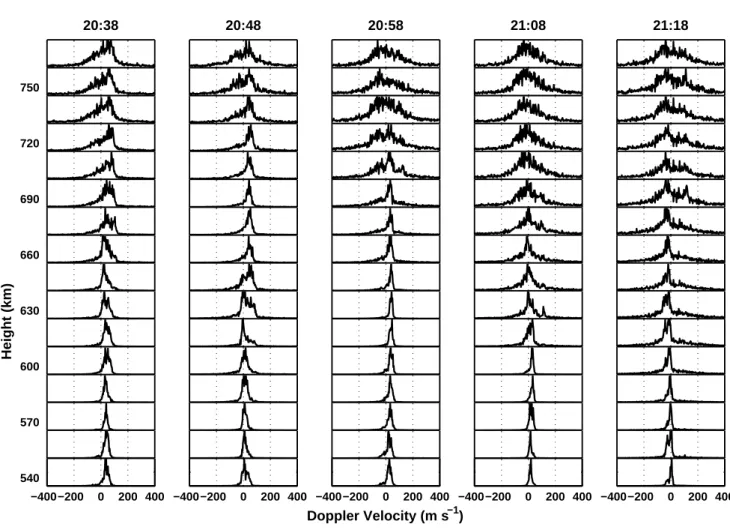
−400−200 0 200 400 540 570 600 Height (km) 630 660 690 720 750 20:38 −400−200 0 200 400 20:48 −400−200 0 200 400 Doppler Velocity (m s−1) 20:58 16 March 1999 −400−200 0 200 400 21:08 −400−200 0 200 400 21:18
Fig. 1. A sequence of Doppler spectra of the 8.3-m ESF irregularities observed on 16 March 1999.
Table 1. Radar parameters and other specifications used for the
spread F experiment’s Parameter.
Parameter value
Frequency 18 MHz
Peak transmitted power 50 kW
Beam Zenith
Beam width (one way) 6.3◦
Pulse repetition frequency 100 Hz
Pulse width 100 µs
Number of FFT points 256
No. of online spectral averaging 16
No. of range bins sampled 32
Height resolution 15 km
Velocity resolution 3.25 ms−1
3 Observations and discussion
The observations of the 8.3-m ESF irregularities presented here were made in equinoctial periods during 1998–2000.
We operated the radar on 40 nights and out of 40 observa-tional runs, ESF irregularities were observed on 27 nights. In the following, we present the observations both episodi-cally and statistiepisodi-cally.
3.1 Doppler spectrum
In Fig. 1, we present a sequence of Doppler power spec-tra on 16 March 1999 corresponding to an altitude range of 540–765 km. The time mentioned on each figure is in In-dian Standard Time (IST) corresponding to 82.5◦ east
lon-gitude. The spectra are generated through online spectral averaging of 16 spectra leading to time averaging of 41 s. The spectra represent the velocity fields enclosed by a radar pulse volume defined by the pulse length of 15 km and a two-way beam-width of 4.4◦and time averaging of 41 s. It may be noted that the velocity spectra are well behaved and confined within the Doppler window limit of ±415 m s−1. Positive/negative Doppler velocity in these figures repre-sents downward/upward phase velocity of the irregularities. Most of the spectra are found to have a width of less than 100 ms−1. Furthermore the lower altitude (< 600 km)
100 300 500 700 900 7 March 1999 (A p = 22) 8 March 1999 (A p = 12) SNR (dB) −12 −9 −6 −3 0 3 6 9 12 13 March 1999 (A p = 6) 100 300 500 700 900 14 March 1999 (A p = 15) 16 March 1999 (A p = 3) 19 March 1999 (A p = 6) 100 300 500 700 900 20 March 1999 (A p = 5) 10 April 1999 (A p = 16) 12 April 1999 (A p = 8) 18 20 22 24 100 300 500 700 900 13 April 1999 (A p = 3)
Height (km)
Time (hrs)
18 20 22 24 14 April 1999 (A p = 7)Time (hrs)
18 20 22 24 19 April 1999 (A p = 12)Time (hrs)
Fig .2. H eight tim e in tensit y pl ots for 12 ev ents (d ates and Ap indi ces are ment ioned on top of each pa nel). Horiz ontal blac k b ar represe nts the dura tion o f ESF as see n by ionoso nde. C ontinu ous and das hed li nes sh o w the v aria tion o f h’F b efore the on set an d duri ng ES F resp ecti v ely .100 300 500 700 900 7 March 1999 (A p = 22) 8 March 1999 (A p = 12) Velocity (m s −1 ) − 100 − 75 − 50 − 25 0 25 50 75 100 13 March 1999 (A p = 6) 100 300 500 700 900 14 March 1999 (A p = 15) 16 March 1999 (A p = 3) 19 March 1999 (A p = 6) 100 300 500 700 900 20 March 1999 (A p = 5) 10 April 1999 (A p = 16) 12 April 1999 (A p = 8) 18 20 22 24 100 300 500 700 900 13 April 1999 (A p = 3)
Height (km)
Time (hrs)
18 20 22 24 14 April 1999 (A p = 7)Time (hrs)
18 20 22 24 19 April 1999 (A p = 12)Time (hrs)
Fig . 3. H eight time v elocity maps corre spond ing to the ev ents sho wn in Fig. 2.spectra are in general narrower and much more consistent in both space and time as compared to the upper region (>600 km). It may be noted that for altitudes >600 km, the spectral width increases as a function of time and finally, at 21:18 IST, the spectra become double-peaked. This indicates the advection of scattering irregularities with a velocity field much different from the previous ones in the radar pulse vol-ume.
Only observations on the spectral characteristics available for comparison at this frequency are that made by Cleme-sha (1964). He has measured spectral width of the order of 40 ms−1and in some extreme cases as high as 70 ms−1. His measurement resolution, however, are not comparable because he used a much wider pulse width (45-km range res-olution). But the point we wish to stress here is that even with such poor resolution measurements, the spectral width was found to be comparable to that measured here. We have not observed a large variety of shapes similar to those observed at Jicamarca by Woodman and LaHoz (1976), who have re-ported spectral widths ranging from a few Hz to as high as 200 Hz (corresponding to 600 m s−1). It may be mentioned
that such wide spectra were observed with a pulse width of 2.5 km and beam-width of 0.7◦ when spectral averaging was performed for 20 s. It may be mentioned that Doppler spectra were measured at ∼50 MHz over Trivandrum in the early seventies (Balsley et al., 1972) and were found to have spectral width of the same order of that shown by Wood-man and LaHoz (1976). Patra et al. (1997) have presented spectra corresponding to 2.8-m scale ESF irregularities ob-served over Gadanki (13.5◦N, 79.2◦E, dip latitude 6.3◦N), India, a low-latitude station just outside the electrojet. They have shown that the spectra are not as variable as they are at Jicamarca. The spectral widths observed by them are less than 150 ms−1. Our observations at Trivandrum suggest that
8.3-m scale irregularities in general display much narrower spectral width as compared to those of 3 m observed over the magnetic equator at Jicamarca and are less than that of Gadanki, which is located in nearly the same longitudinal sector over India.
3.2 Height-time-intensity map
Intensity maps of 12 ESF events observed during March-April 1999 are shown in 12 panels in Fig. 2 to illustrate the types of ESF structures that we observed. These figures are so-called height-time-intensity maps in which the intensity represents a signal-to-noise ratio (SNR). SNR computation has been done using the averaged Doppler Power spectra, as mentioned in the previous section. This permits us to mea-sure SNR accurately down to about 15 dB. During this pe-riod, the Ap index varied from 3–22 (Ap values are
men-tioned on each panel). In the above figures, the thin, con-tinuous lines represent the time history of the F-layer height before the onset of ESF, as observed in the ionograms. The thin dashed lines represent the time history of the approxi-mate height of the F-layer. This only gives us some idea on how the F-layer height might be changing as a function of
time and also from one day to the next. The thick horizontal bars represent the duration of ESF as observed in ionograms. It may be noted that the ESF irregularities are initiated at a time when the F-layer height has gone up to about 300 km or more, and is about to reverse direction, as expected (e.g. Hysell and Burcham, 1998). Further, it may be noted, in general, that the diffuse echoes detected in ionograms always precede the ESF echoes observed by the 18 MHz radar. On average, there is a delay of 15–30 min in the occurrence of 8.3-m backscatter as compared to 15-m to 150-m scale size irregularities that are observed typically by a ionosonde. This is quite expected in view of the fact that the small-scale irreg-ularities are generated through a cascade from larger scale sizes following a hierarchy of processes (Haerendel, 1973). Part of this time difference, however, is connected to the sen-sitivity of the two systems and the scattering cross section of the different scale sizes.
Observations suggest that in most of the cases, we have seen one to three plumes. Periodic multiple plume struc-tures, which are common at Jicamarca, Kwajalein (8.8◦N, 167.5◦E, dip latitude 4.3◦N), as well as at Gadanki, are not seen here. It appears that not observing more than three plumes and especially no high altitude plumes in the mid-night and post-midmid-night hours seems to be due to a lack of sensitivity of the radar system in relation to the 8.3-m irreg-ularities. Post-midnight plumes seen are those confined to altitudes less than 500 km, as observed on 20 March and 10 April. It is expected that during the later part of the evening, the ESF development will be rather slow due to a lack of turbulence at this wavelength.
Bottomside irregularities are also not a common feature on all the days, unlike that reported for the 3-m irregulari-ties observed at Jicamarca (e.g. Woodman and LaHoz, 1976). The bottomside layers are commonly observed even when plumes are not observed, and the bottomside irregularities always precede the plume structures at Jicamarca, as seen by the 50 MHz Jicamarca radar. Similar results have also been seen by the CUPRI operated from Alcantara (2.3◦S, 44.4◦W, dip latitude 0.7◦S), Brazil (Swartz and Woodman, 1998). But the bottomside structures are rarely observed at Kwajalein and Gadanki. It may be mentioned that both the places correspond to a low latitude of ∼6◦ geomagnetic lati-tude. Accordingly, the bottomside structures observed at the equator are not expected to map to low latitude. The struc-tures above about 350 km only will be able to map to low latitude and will be observed at altitudes above 250 km. The fact that they have not been observed at Kwajalein and at Gadanki is due to the low altitude confinement of the bot-tomside layers at the equator. Out of 12 events shown here, the bottomside irregularities seem to be present in 5 examples (7, 8, 13, 14 March, 10 April). It may be noted in general that the bottomside echoes are weaker as compared to those as-sociated with the plumes. This is also the case with the 3-m echoes observed so extensively at Jicamarca (Woodman and LaHoz, 1976). SNR in these examples are found to be in the range of 15 to 25 dB, and are found to be quite comparable to those reported from Alcantara using the CUPRI system
(Swartz and Woodman, 1998). We present more statistics on this aspect later, based on the entire database of 27 observa-tional runs at Trivandrum and make a detailed comparison with that reported at other locations. Furthermore, the ob-servations seem to indicate the effect of geomagnetic activity as another important aspect of study. During high solar flux conditions, geomagnetic activities generally suppress the oc-currence of the irregularities (Bowman, 1987) and nearly ar-rest the occurrence of plumes (see, for example, the RTI map of 7 March 1999). This, however, cannot be studied with the limited observations presented here.
3.3 Doppler velocity
In Fig. 3, we present the vertical Doppler velocities, which represent the phase velocities, corresponding to the exam-ples shown in Fig. 2. These represent the gross features in the velocity maps of the ESF irregularities. We know from the earlier experience of the 3-m ESF irregularities that spec-tral observations of ESF are often found to be difficult, since the radar target is often overspread. We, however, have not faced any such difficulty in the observations at 8.3 m. To our surprise we have not seen highly structured echoes like that of 3 m observed so extensively. The echoes that we have ob-served at 8.3 are relatively narrow and less structured. So the estimation of the mean Doppler velocity is quite satis-factory and the Doppler velocity is a good representation of the mean phase velocities of the 8.3-m irregularities. It may be noted that most of the Doppler velocities lie in the range
±100 ms−1. It may be mentioned that the velocities have not suffered from aliasing. The pulse repetition frequency used in these experiments is 100 Hz, which correspond to Doppler velocity limit of ±415ms−1. We believe that the
ve-locities are not aliased veve-locities due to the fact that in such case, Doppler velocities would go through a smooth transi-tion in which the values would change from zero through
∼400 ms−1and go to the negative Doppler domain or vice versa. This, however, has not been noted in our data.
On 7 March, the Doppler velocities are downward only and no spread F echoes have been observed beyond the peak of the F-layer. This day happened to be a magnetically mod-erately disturbed day (Ap=22). On other days, however,
both upward and downward velocities have been observed and irregularities have been seen to penetrate to the top of the F-region. It may be noted that most of the topside structures have dominant upward velocities and lower altitude echoes have downward velocities. This is quite expected in the F-region due to the fact that the velocities are mainly controlled by the electric field below about 350 km and by the buoy-ancy force (g/vin; where g is the gravitational acceleration
and vinis the collision frequency between the ions and the
neutrals) above (Ossakow and Chauturvedi, 1978; Anderson and Haerendel, 1979). Since the night-time background elec-tric field is westward at the time of the ESF observations, the dominant downward velocities observed at the lower alti-tudes basically represent the zonal electric field. We present
Table 2. A list of dates and magnetic conditions corresponding to
the ESF observations.
S. No. Date Ap 1 23 March 1998 6 2 24 March 1998 7 3 25 March 1998 16 4 30 March 1998 8 5 17 April 1998 15 6 18 April 1998 6 7 19 April 1998 4 8 20 April 1998 10 9 21 April 1998 7 10 22 April 1998 6 11 7 March 1999 22 12 08 March 1999 12 13 13 March 1999 6 14 14 March 1999 15 15 16 March 1999 3 16 19 March 1999 6 17 20 March 1999 5 18 10 April 1999 16 19 12 April 1999 8 20 13 April 1999 3 21 14 April 1999 7 22 19 April 1999 12 23 10 August 1999 5 24 11 August 1999 6 25 11 September 2000 4 26 28 September 2000 12 27 29 September 2000 7
more statistics later and compare these with that observed so extensively for the 3-m scale size.
3.4 Statistical characteristics
While most of the characteristics of the 8.3-m ESF irregular-ities could be recognized from the presentation given in the previous section, it is more appropriate and useful to have statistical results. This helps us in comparing the character-istics observed at 8.3 m with those of 3 m. These statistical characteristics are based on the database of 27 night-time ob-servations. The dates and the corresponding magnetic condi-tions of these observacondi-tions are given in Table 2.
In Fig. 4a, we present the percentage occurrence of the 8.3-m ESF irregularities as function of height and time. In Fig. 4b, we present the percentage occurrence of ESF ir-regularities as observed by a collocated ionosonde (contin-uous line) and the maximum percentage occurrence of 8.3-m irregularities observed by the 18 MHz radar (dashed line). It may be noted that the ESF irregularities started occur-ring at the time when the electric field is believed to reverse from eastward to westward. The irregularities are found to reach to high altitudes mostly during 19:15–20:15 IST and have reached to altitudes as high as 1200 km. We have not
0 20 40 60 80 100 18 19 20 21 22 23 24 01 200 400 600 800 1000 1200 Height (km)
(a) % Occurrence of ESF in radar observations
18 19 20 21 22 23 24 01 20 40 60 80 100 Time (hrs) Percentage (%)
(b) Maximum % Occurrence of radar echoes and % Occurrence of spread F on Ionogram
Fig. 4. (a) Height time distribution of percentage occurrence of 8.3-m ESF irregularities and (b) percentage occurrence of ESF irregularities
as observed by ionosonde (continuous line) and maximum percentage occurrence of 8.3-m ESF irregularities as observed by radar (dashed line).
seen late-night plasma plumes extend to altitudes higher than 500 km (for example, see the RTI on 20 March and 10 April in Fig. 2). It may be mentioned that the bottomside irreg-ularities occur immediately after the first plumes took over (Hysell and Burcham, 1998) and they generally do not reach to very high altitudes. Based on the 27 observational runs, we see that the occurrence of 8.3-m ESF irregularities maxi-mizes at about 20:30 IST at an altitude close to 600 km. The ESF occurrence is found to be <20% before 20:00 IST and after ∼22:00 IST, >20% during 20:00–22:00 IST and >40% only during 20:15–21:15 IST. Furthermore, the occurrence of very high altitude irregularities is only 20% and less.
Figure 4b shows the percentage occurrence of ESF irregu-larities seen by ionosonde and the maximum percentage oc-currence of ESF. Irregularities seen by the ionosonde precede the radar observations and also continue for a long time after the disappearance of the signals in the radar. It may be men-tioned that the scale sizes responsible for the backscatter in case of ionosode frequencies are larger than that of the radar. Although the sensitivity of the two systems and the scatter-ing cross sections at different scale sizes are important for their detection in the two systems, the late occurrence of the
8.3-m irregularities could be attributed to the hierarchy of in-stability processes (large scales appearing first and cascading down to small scales) (Haerendel, 1973).
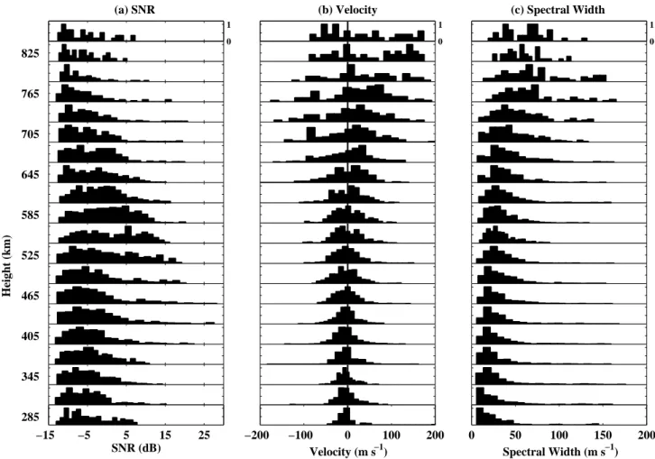
In Figs. 5a–c, we present the spectral parameters viz. SNR, mean Doppler velocity and spectral width in the form of a histogram. The above parameters correspond to an alti-tude range of 185–855 km. It may be noted that SNR could be as high as 25 dB and we could detect a signal down to
∼−15 dB. Accordingly, the strongest signal is approximately 40 dB above the noise level. But most of the SNRs are con-fined to 15 and 15 dB, and the strongest signals are observed in the altitude range of 400–600 km. This height region hap-pened to be the neck of the plume structures (e.g. Woodman and LaHoz, 1976), where the turbulence is expected to be more. It may be mentioned that the SNR observed at Trivan-drum, using a 54.95 MHz system of almost equal sensitivity, was found to be of the same order (Rao et al., 1997) The ob-servations reported by Rao et al. (1997) were made by point-ing the radar beam at a zenith angle of 30◦due west. The ob-served SNR is also comparable to that reported by Hysell et al. (1994) and Swartz and Woodman (1998) from Kwajalein and Alcantara using the CUPRI, a comparable radar system.
−15 −5 5 15 25 SNR (dB) 285 −200 −100 0 100 200 Velocity (m s−1) 0 50 100 150 200 Spectral Width (m s−1) 345 405 465 Height (km) 525 585 645 705 765 825 0 1 (a) SNR 0 1 (b) Velocity 0 1 (c) Spectral Width
Fig. 5. Histograms of (a) SNR, (b) velocity and (c) spectral width as function of height for 8.3 m ESF irregularities. Histograms are generated
from 66 h of data arising from 27 observational runs.
Between Alcantara and Kwajalein, however, the ESF mor-phologies are different. At Kwajalein, no bottomside struc-tures were observed unlike at Alcantara. The fact that we have not seen the bottomside structures on every night using the 18-MHz system seems to be due to the low sensitivity of the system. It may be mentioned that the sky noise is about 10 dB higher at 18 MHz as compared to 50 MHz. We believe that this is the main reason why we are not able to detect the weaker echoes associated with the bottomside structures. These echoes have been observed regularly using the Jica-marca radar with SNR exceeding 30 dB (Woodman and La-Hoz, 1976). The system we used is about 20 dB less sensitive than the Jicamarca radar. We believe that the low sensitivity and the sky noise are responsible for not observing the bot-tomside structures on a regular basis.
The Doppler velocities presented in Fig. 5b are confined within ±200 ms−1. Positive (negative) velocities represent upward (downward) phase velocities of the irregularities. It may be noted that up to an altitude of about 600 km, the velocities are within 100 ms−1 and highly organized. The velocity distributions are symmetric about zero. Above this height, the velocities are more and generally upward. This is quite expected due to the nonlinear growth of the
Rayleigh-Taylor instability (e.g. Zalesak et al., 1982) and also due to the dominant role of the buoyancy force resulting from di-minishing collision as a function of height (e.g. Ossakow and Chaturvedi, 1978). The observed velocities, however, are less as compared to those observed for 3 m, both at the dip equator (e.g. Woodman and LaHoz, 1976; Hysell and Bur-cham, 1998), as well as at low latitudes (Hysell et al., 1994; Rao et al., 1997). The velocities associated with the topside irregularities observed by them often exceeded 300 ms−1.
In Fig. 5c, we present the spectral widths which are well within 150 ms−1and most of the values lie below 100 ms−1. It may be noted that most of the spectral widths below
∼600 km are within 50 ms−1. It is surprising to note that, in
this altitude region, the spectral widths are found to be so low even for the strongest signals. Spectral widths have been ob-served to be as high as 600 ms−1at ∼3 m, both at Jicamarca and at Trivandrum (Woodman and LaHoz, 1976; Balsley et al., 1972). Spectral widths observed at Gadanki (Patra et al., 1997) are also higher than the values observed here. It may be mentioned that the observations for 8.3-m scale size ESF irregularities here were made using a wider beam than that of Jicamarca and Gadanki. Accordingly, we would expect larger spectral width, since the volume encompassed by the
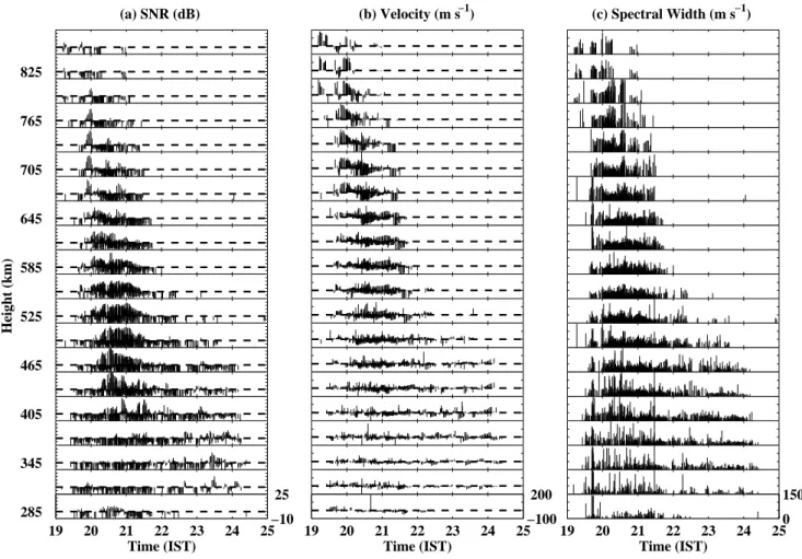
19 20 21 22 23 24 25−10 25 Time (IST) 285 19 20 21 22 23 24 25−100 200 Time (IST) 19 20 21 22 23 24 250 150 Time (IST) 345 405 465 Height (km) 525 585 645 705 765 825
(a) SNR (dB) (b) Velocity (m s−1) (c) Spectral Width (m s−1)
Fig. 6. Temporal variations of (a) SNR, (b) velocity and (c) spectral width as a function of height for 8.3-m ESF irregularities. The figures
are generated using 66 h of data arising from 27 observational runs.
beam is large and hence, the beam broadening effect on the measured spectral width is expected to be more. The obser-vations, however, show lesser values as compared to those of 3 m, indicating the lifetime of 8.3-m irregularities to be larger than that of 3-m (Woodman and La Hoz, 1976; Patra et al., 1997). Furthermore, it may be noted that mean Doppler ve-locity plus the spectral width even in the extreme case does not exceed the observational Doppler limit of ±415 ms−1.
In Figs. 6a–c, we present the height time variations of the three spectral parameters (SNR, velocity and spectral width). We have plotted the SNR values lying within 10 and 25 dB. It may be noted that the strongest signals are observed during 20:30–21:30 IST when ESF bubbles are expected to rise. At the later phase of the ESF, the SNR is found to be low. These features indicate the role of the background electric field on the growth of the ESF irregularities. During the later phase, in the presence of background westward electric field, the ESF development is inhibited.
In Fig. 6b, it may be noted that during the growth phase of the ESF, during 20:30–21:30 IST, the velocities are dom-inantly upward, reaching values as high as 200 ms−1. At the later phase, however, very small velocities, both up-ward and downup-ward are present. While on the bottomside,
the velocities are both upward and downward and are small (<±50 ms−1), they are mostly upward and higher in magni-tude on the topside. Since buoyancy is not dominant below 400 km, the velocities could be used as a good representation of the zonal electric field during the spread F conditions.
In Fig. 6c, the spectral width variations show that the widest spectral widths are associated with the growth phase of the ESF and mostly confined to the topside of the F-layer. A more careful inspection of the database suggests that very strong signals are not always associated with the widest spec-tral width.
From the above presentation, we can summarize the re-sults as follows:
1. The Doppler spectra observed for the 8.3-m ESF irregu-larities are found to be narrower and less structured than those reported for 3 m.
2. The RTI maps show that, in general, one to three plume structures are observed in contrast to multiple periodic plumes observed at 3 m.
3. The percentage occurrence of the 8.3-m ESF irregular-ities are found to be <20% before 20:00 IST and after
∼22:00 IST, >20% during 20:00–22:00 IST and >40% only during 20:15–21:15 IST.
4. The 8.3-m irregularities have been seen to occur at alti-tudes as high as 1200 km on some occasions.
5. The Doppler velocity and spectral width are well within
±200 ms−1and 150 ms−1, respectively.
Among the above observations, what is more remarkable is the Doppler velocities and spectral widths of 8.3 m be-ing much less compared to those reported for 3 m. It may also be noted that both the parameters added together do not exceed the observational Doppler limit of ±415 ms−1. So we can say that the velocities are not ambiguous, and the low values of Doppler velocities and the spectral width are the characteristic features of the 8.3-m scale ESF irregulari-ties. A Doppler velocity exceeding 1000 ms−1has been ob-served both at Jicamarca and Kwajalein (Hysell et al., 1994). Satellite-borne measurements also show plasma flow to be supersonic (Aggson et al., 1992). Hysell et al. (1994), based on their observations, interpreted these Doppler velocities as the guiding center drifts. Large Doppler velocities have also been observed using a newly installed 30 MHz radar in Brazil (dePaula et al. (2002), results presented in Jicamarca Work-shop). They have shown that quite often, the topside veloc-ities exceed 300 ms−1. It appears that the Doppler velocity, as well as the spectral width observed in the American sec-tor, are larger than that of the Indian sector. This statement, however, cannot be generalized in view of the fact that, for a detailed comparison, we need to have a statistically stronger database, which we wish to have in the future.
In this context, it may be mentioned that, in general, the background plasma drift in the Indian sector is less than the American sector (Namboothiri et al., 1989; Viswanathan et al., 1992; Hari and KrishnaMurthy, 1995). Viswanathan et al. (1992) have shown that the daytime values of verti-cal drifts at Trivandrum, as measured by a HF radar, are smaller than those observed at Jicamarca by a factor of ∼1.5. Hari and Krishna Murthy (1995) have compared the vertical drifts at Trivandrum and Jicamarca for the post sunset period. Their results show that post sunset peak values of upward drifts are greater at Jicamarca than those at Trivandrum in equinox and summer months, whereas in winter the situation is the opposite. The night-time downward drift is also greater at Jicamarca than that at Trivandrum during all the seasons by as much as a factor of 2 during some hours. From the electrojet strength measurements at Jicamarca and at Trivan-drum, Sinha et al. (1999) have come to the same conclusion and have shown that the cowling conductivity ratio for the American sector over the Indian sector is about 1.73. In view of the above fact we wonder whether the general tendency of observing low velocities in the Indian sector is due to this asymmetry of background vertical drift of the F-region in the two sectors. This, however, needs to be established with a larger database than that reported here, especially from the viewpoint of 8.3-m versus 3-m irregularities.
4 Concluding remarks
In this paper, we presented a comprehensive picture of the characteristics of the 8.3-m ESF irregularities observed using the new 18 MHz radar over Trivandrum. The observations clearly suggest that velocity and spectral width observed for 8.3-m scale irregularities are smaller than that of 3 m. We have not observed velocities and spectral width more than 200 ms−1and 150 ms−1respectively. Further, the velocities are less than those observed in the American sector, which we attributed to the role of different background electric field prevailing in the two sectors. The velocities observed above 400 km, where the nonlinear plasma dynamics and the buoy-ancy force are believed to be dominant, are also less than those of the American sector. We wish to study this aspect more carefully with a larger database than the one used here. The observed velocities at the lower altitudes (<400 km) are comparable to the background plasma drift suggesting that 8.3-m scale irregularities could be used to measure the zonal electric field during spread F conditions.
Acknowledgements. The 18 MHz radar belongs to and operated by
Space Physics Laboratory, Vikram Sarabhai Space Centre. We are grateful to the engineering staff without whose support the observa-tions presented here would not have been made possible. The work is supported by Department of Space.
Topical Editor M. Lester thanks S. Basu for the help in evaluat-ing this paper.
References
Aggson, T. L., Burke, W. J., Maynard, N. C., Hanson, W. B., An-derson, P. C., Slavin, J. A., Hogey, W. R., and Saba, J. L.: Equa-torial bubbles updrafting at supersonic speeds, J. Geophys. Res., 97, 8581, 1992.
Balsley, B. B., Haerendel, G., and Greenwald, R. A.: Equatorial spread F: Recent observations and a new interpretation, J. Geo-phys. Res., 77, 5625, 1972.
Basu, S., MacKenzie, E., Basu, S.: Ionospheric constraints on VHF/UHF communication links during solar maximum and min-imum periods, Radio Sci., 23, 363, 1988.
Berkner, L. V., and H. W. Wells, F-region ionospheric investigation at low latitudes, Terrestrial Magnetism, 39, 215, 1934.
Bowman, G. G.: Some effects of geomagnetic activity on spread-F occurrence and ionospheric height variations in equatorial re-gion, J. Atmos. Solar Terr. Phys. 49, 19, 1987.
Cecile, J. F., Vila, P., and Blanc, E.: HF radar observations of equa-torial spread F over west Africa, Ann. Geophysicae, 14, 411, 1996.
Clemesha, B. R.: An investigation of the irregularities in F-region associated with equatorial type spread F, J. Atmos. Terr. Phys. 26, 91, 1964.
Dyson, P. L. and Benson, R. F.: Topside sounder observations of equatorial bubble, Geophys. Res. Lett., 5, 795, 1978.
dePaula, E. R., Hysell, D. L., and Rodrigues, F. S.: The Sao-Luis VHF coherent backscatter ionospheric radar results during solar maximum, paper presented at Jicamarca Workshop during May 20–23, 38, 2002.
Farley, D. T., Balsley, B. B., Woodman, R. F., and McClure, J. P.: Equatorial spread F: Implications of VHF radar observations, J. Geophys. Res., 75, 7199, 1970.
Farley, D. T. and Hysell, D. L.: Radar measurements of very small aspect angles in the equatorial ionsophere, J. Geophys. Res., 101, 5177, 1996.
Hari, S. S. and KrishnaMurthy, B. V.: Equatorial night-time F-region zonal electric field, Ann. Geophys., 13, 871, 1995. Haerendel, G.: Theory of equatorial spread F, Max-Planck Institute
f¨ur Physik und Astrophysik, Garching, West Germany, 1973. Hanson, W. B. and Bamgboye, D. K.: The measured motions inside
equatorial plasma bubbles, J. Geophys. Res., 89, 8997, 1985. Hysell, D. L., Kelley, M. C., Swartz, W. E., and Farley, D. T.: VHF
radar and rocket observations of equatorial spread F on Kwa-jalein, J. Geophys. Res., 99, 15 065, 1994.
Hysell, D. L. and Woodman, R. F.: Imaging coherent backscatter radar observations of topside equatorial spread F, Radio Sci., 32, 2309, 1997.
Hysell, D. L. and Burcham, J.: JULIA radar studies of equatorial spread F, J. Geophys. Res., 103, 29 155, 1998.
Janardhanan, K. V., Ramakrishna Rao, D., Viswanathan, K. S., Kr-ishna Murthy, B. V., Shenoy, K. S. V., Mohan Kumar, S. V., Ka-math, K. P., Mukundan, K. K., Sajitha, G., Shajahan, M., and Ayyappan, C.: HF backscatter radar at the magnetic equator: System details and preliminary results, Indian J. Radio and Space Phys., 30, 77, 2001.
Jayachandran, B., Balan, N., Namboothiri, S. P., and Rao, P. B.: HF Doppler observations of vertical plasma drifts in the evening F-region at the equator, J. Geophys. Res., 92, 11 253, 1987. Kelley, M. C., LaBelle, L., Kudeki, E., Fejer, B. G., Basu, Sa., Basu,
Su., Baker, K. D., Hanuise, C., Agro, P., Woodman, R. F., Swartz, W. E., Farley, D. T., and Meriwether Jr., J. W.: The Condor equa-torial spread F campaign: overview and results of the large-scale measurements, J. Geophys. Res., 91, 5487, 1986.
Kelleher, R. F. and Skinner, N. J.: Studies of F-region irregularities at Nairobi II–By direct backscatter at 27.8 MHz, Ann. Geophys., 27, 195, 1971.
McClure, J. P., Hanson, W. B., and Hoffman, J. H.: Plasma bubbles and irregularities in the equatorial ionosphere, J. Geophys. Res., 82, 2650, 1977.
Mendillo, M. and Baumgardner, J.: Airglow characteristics of equa-torial plasma depletions, J. Geophys. Res., 87, 7641, 1982. Namboothiri, S. P., Balan, N., and Rao, P. B.: Vertical plasma drifts
in the F-region at the magnetic equator, J. Geophys. Res., 94, 12 055, 1988.
Ossakow, S. L. and Chaturvedi, P. K.: Morphological studies of rising equatorial spread F bubbles, J. Geophys. Res., 83, 2085, 1978.
Patra, A. K., Rao, P. B., Anandan, V. K., and Jain, A. R.: Radar observations of 2.8 m equatorial spread F irregularities, J. Atmos. Solar Terr. Phys. 59, 1633, 1997.
Pfaff, R. F., Sobral, J. H. A., Abdu, M. A., Swartz, W. E., Labelle, J. W., Larsen, M. F., Goldberg, R. A., and Schimidlin, F. J.: The Guara Campaign: A series of rocket-radar investigations of the
earth’s upper atmosphere at the magnetic equator, Geophys. Res. Lett., 24, 1663, 1997.
Rao, P. B., Patra, A. K., Chandrasekhar Sharma, T. V., Krishna Murthy, B. V., Subbarao, K. S. V., and Hari, S. S.: Radar ob-servations of updrafting and downdrafting plasma depletions as-sociated with equatorial spread F, Radio Sci., 32, 1215, 1997. Reddy, C. A., Janardhanan, K. V., Mukundan, K. K., and Shenoy, K.
S. V.: Concept of an interlaced phased array for beam switching, IEEE, Transactions on antennas and propagation, 38, 573, 1990. Sahr, J. D., Farley, D. T., and Swartz, W. E.: Removal of aliasing in pulse-to-pulse Doppler radar measurements, Radio Sci., 24, 697, 1989.
Sekar, R., Kherani, E. A., Viswanathan, K. S., Patra, A. K., Rao, P. B., Devasia, C. V., Subbarao, K. S. V., Tiwari, D., and Ra-machandran, N.: Preliminary results and equatorial spread F ir-regularities by VHF and HF radars, Indian J. Radio and Space Phys., 29, 262, 2000.
Sinha, H. S. S., Rajesh, P. K., Mishra, R. N., and Dutt, N.: Multi-wavelength imaging observations of plasma depletion over Kavalur, India, Ann. Geophys., 19, 1119, 2001.
Sinha, H. S. S., Chandra, H., and Rastogi, R. G.: Longitudinal in-equalities in the equatorial electrojet, Proc. Nat. Acad. Sci, India, 69(A), I, 1999.
Sinha, H. S. S., Raizada, S. and Mishra, R. N.: First simultaneous in situ measurement of electron density and electric field fluctu-ations during spread F in the Indian zone, Geophys. Res. Lett., 20, 1669, 1999.
Swartz, W. E. and Woodman, R. F.: Same night observations of spread F by the Jicamarca Radio observatory in Peru and CUPRI in Alcantara, Brazil, Geophys. Res. Lett., 25, 17, 1998. Szuszczewicz, E. P., Tsunoda, R. T., Narcisi, R., and Holmes, J. C.:
Coincident radar and rocket observations of equatorial spread F, Geophys. Res. Lett., 7, 537, 1980.
Towel, D. M.: VHF and UHF radar observations of equatorial F-region ionospheric irregularities and background densities, Radio Sci., 15, 71, 1980.
Tsunoda, R. T.: Backscatter measurements of 11 cm equatorial spread F irregularities, Geophys. Res. Lett., 7, 848, 1980. Tsunoda, R. T., Barton, M. J., Owen, J., and Towle, D. M.: Altair
incoherent scatter radar for equatorial spread F studies, Radio Sci., 14, 1111, 1979.
Viswanathan, K. S., Namboothiri, S. P., and Rao, P. B.: VHF and HF radar measurements of E- and F-region plasma drifts at the magnetic equator, J. Geophys. Phys., 97, 3011, 1992.
Weber, E. J., Buchau, J., Eather, R. H., and Mende, S. B.: North-south field aligned equatorial airglow depletions, J. Geophys. Res., 83, 712, 1978.
Woodman, R. F. and LaHoz, C.: Radar observations of F-region equatorial irregularities, J. Geophys. Res., 81, 5447, 1976. Woodman, R. F.: Spectral moment estimation in MST radars, Radio
Sci., 20, 1185, 1985.
Zalesak, S. T., Ossakow, S. L., and Chaturvedi, P. K.: Nonlinear equatorial spread F: The effect of neutral winds and background Pedersen conductivity, J. Geophys. Res., 87, 151, 1982.