HAL Id: hal-00360906
https://hal.archives-ouvertes.fr/hal-00360906
Submitted on 2 Jan 2016
HAL is a multi-disciplinary open access
archive for the deposit and dissemination of
sci-entific research documents, whether they are
pub-lished or not. The documents may come from
teaching and research institutions in France or
abroad, or from public or private research centers.
L’archive ouverte pluridisciplinaire HAL, est
destinée au dépôt et à la diffusion de documents
scientifiques de niveau recherche, publiés ou non,
émanant des établissements d’enseignement et de
recherche français ou étrangers, des laboratoires
publics ou privés.
mesosphere humidity analyses
H.E. Thornton, D.R. Jackson, Slimane Bekki, N. Bormann, Q. Errera, A.J.
Geer, W.A. Lahoz, S. Rharmili
To cite this version:
H.E. Thornton, D.R. Jackson, Slimane Bekki, N. Bormann, Q. Errera, et al.. The ASSET
intercom-parison of stratosphere and lower mesosphere humidity analyses. Atmospheric Chemistry and Physics,
European Geosciences Union, 2009, 9 (3), pp.995-1016. �10.5194/acp-9-995-2009�. �hal-00360906�
www.atmos-chem-phys.net/9/995/2009/
© Author(s) 2009. This work is distributed under the Creative Commons Attribution 3.0 License.
Chemistry
and Physics
The ASSET intercomparison of stratosphere and lower mesosphere
humidity analyses
H. E. Thornton1, D. R. Jackson1, S. Bekki2, N. Bormann3, Q. Errera4, A. J. Geer3, W. A. Lahoz5, and S. Rharmili2 1Met Office, UK
2UPMC Univ Paris 06; CNRS; SA-IPSL, France
3European Centre for Medium-Range Weather Forecasts, UK 4Insitut d’A´eronomie Spatiale de Begique, BIRA-IASB, Belgium 5Norsk Institutt for Luftforskning, Norway
Received: 8 April 2008 – Published in Atmos. Chem. Phys. Discuss.: 15 July 2008 Revised: 6 January 2009 – Accepted: 6 January 2009 – Published: 9 February 2009
Abstract. This paper presents results from the first de-tailed intercomparison of stratosphere-lower mesosphere wa-ter vapour analyses; it builds on earlier results from the EU funded framework V “Assimilation of ENVISAT Data” (AS-SET) project. Stratospheric water vapour plays an impor-tant role in many key atmospheric processes and therefore an improved understanding of its daily variability is desir-able. With the availability of high resolution, good quality Michelson Interferometer for Passive Atmospheric Sounding (MIPAS) water vapour profiles, the ability of four different atmospheric models to assimilate these data is tested. MI-PAS data have been assimilated over September 2003 into the models of the European Centre for Medium Range Weather Forecasts (ECMWF), the Belgian Institute for Space and Aeronomy (BIRA-IASB), the French Service d’A´eronomie (SA-IPSL) and the UK Met Office. The resultant middle atmosphere humidity analyses are compared against inde-pendent satellite data from the Halogen Occultation Exper-iment (HALOE), the Polar Ozone and Aerosol Measurement (POAM III) and the Stratospheric Aerosol and Gas Experi-ment (SAGE II). The MIPAS water vapour profiles are gen-erally well assimilated in the ECMWF, BIRA-IASB and SA systems, producing stratosphere-mesosphere water vapour fields where the main features compare favourably with the independent observations. However, the models are less ca-pable of assimilating the MIPAS data where water vapour values are locally extreme or in regions of strong humid-ity gradients, such as the southern hemisphere lower strato-sphere polar vortex. Differences in the analyses can be at-tributed to the choice of humidity control variable, how the background error covariance matrix is generated, the model
Correspondence to: H. E. Thornton ([email protected])
resolution and its complexity, the degree of quality control of the observations and the use of observations near the model boundaries. Due to the poor performance of the Met Office analyses the results are not included in the intercomparison, but are discussed separately. The Met Office results highlight the pitfalls in humidity assimilation, and provide lessons that should be learnt by developers of stratospheric humidity as-similation systems. In particular, they underline the impor-tance of the background error covariances in generating a re-alistic troposphere to mesosphere water vapour analysis.
1 Introduction
The “Assimilation of ENVISAT Data” project (ASSET: http://darc.nerc.ac.uk/asset/; Lahoz et al., 2007) was an EU funded initiative to exploit and develop earth observation data from ENVISAT using data assimilation. ENVISAT was launched in 2002 and is one of the largest Earth Observa-tion (EO) satellites ever built. It carries several sophisticated EO instruments providing insights into the chemistry and dy-namics of the atmosphere. ASSET has co-ordinated the as-similation of different ENVISAT data products into a vari-ety of different atmospheric models, both global circulation models (GCMs) and chemical transport models (CTMs). The resultant analyses therefore can be used to study constituent atmospheric variability and modelling differences. Strato-spheric water vapour analyses have been produced by a num-ber of centres within the ASSET project. This paper sum-marises the differences between the water vapour analyses and how they compare with independent observations. The aim is to summarise the current performance of humidity as-similation schemes, highlighting areas where improvement is required, and quantifying their errors.
Gaining a good knowledge of the daily variability of the water vapour field in the stratosphere is very desirable, as upper troposphere/lower stratosphere (UTLS) water vapour is known to play an important role in many aspects of meteo-rology, including radiation, dynamics, chemistry and climate change (Kley et al., 2000). For example, water vapour is the main source of the hydrogen radicals which are respon-sible for most of the ozone destruction in the lower strato-sphere and it is also a major greenhouse gas in the UTLS. A detailed understanding of the characterisation of the water vapour field and its variability in the UTLS region would also improve our understanding of cirrus clouds and the identifi-cation of the transport pathways between the troposphere and the stratosphere, in particular the relative importance of slow tropical ascent and of deep convection. Our observational knowledge of this daily variability remains relatively poor. Brewer (1949) first reported the extreme dryness of strato-spheric air via aircraft-borne hygrometer observations, but these observations were only made over southern England. In subsequent decades the observational knowledge of strato-spheric water vapour was extended, using balloon-borne frost point hygrometer (e.g. Mastenbrook and Daniels, 1980) and Lyman-alpha hygrometer (e.g. Kley et al., 1979) obser-vations, but these were also only available at a small number of geographical locations. These observations showed that water vapour increased with height in the stratosphere and that a water vapour minimum (the hygropause) existed 2– 3 km above the tropopause (e.g. Kley et al., 1979).
The first global observations of stratospheric water vapour were made by the Limb Infrared Monitor of the Strato-sphere (LIMS) satellite instrument in 1978. These observa-tions provided extended latitudinal coverage (64◦S–84◦N),
confirmed the earlier in-situ hygrometer observations and showed that the hygropause was a general feature of the tropical stratosphere. Subsequently, observations from the Upper Atmosphere Research Satellite (UARS) launched in 1991, including measurements from the Microwave Limb Sounder (MLS), Cryogenic Limb Array Etalon Spectrometer (CLAES) and the Improved Stratospheric and Mesospheric Sounder (ISAMS), made a further important contribution to the observational knowledge of stratospheric water vapour (e.g. Pumphrey et al., 1998). These data were only available for relatively short time periods (6–18 months), but obser-vations of longer-term stratospheric water vapour variability are available from other instruments such as the Halogen Oc-cultation Experiment (HALOE), the Stratospheric Aerosol and Gas Experiment (SAGE II) and the Polar Ozone and Aerosol Measurement experiments (POAM II & III). A par-ticularly important result was reported by Mote et al. (1996), who used HALOE observations to show the influence of tropical tropopause temperatures and stratospheric transport on the equatorial stratospheric water vapour distribution (also known as the “tropical tape recorder”).
Data assimilation is a highly effective method of repre-senting and understanding the daily variability of
meteoro-logical fields (Kalnay, 2003). However, the application of data assimilation to stratospheric water vapour has hitherto been limited by either the lack of reliable humidity data or the lack of well-tested assimilation setups using such data. LIMS and UARS/MLS humidity data were available before humidity assimilation methods became sufficiently well de-veloped, and therefore these data were never, to our knowl-edge, assimilated. The SAGE II and HALOE instruments use solar occultation and therefore have very poor daily spatial sampling of the atmosphere. Therefore, the assimilation of these humidity data would be of minimal use. Currently, the operational assimilation of humidity data in the stratosphere by Numerical Weather Prediction (NWP) centres is limited by the availability of suitable data (Simmons et al., 1999). For example, the quality of humidity observations from ra-diosondes decreases with decreasing water vapour and thus stratospheric water vapour observations from radiosondes are not very useful (Schmidlin and Ivanov, 1998), whilst opera-tional satellite sounders tend to be only sensitive to tropo-spheric water vapour (e.g. the Advanced TIROS Operational Sounder, ATOVS) or total water vapour column (e.g. the Spe-cial Sensor Microwave/Imager, SSM/I). An additional hand-icap to the development of an effective stratospheric water vapour assimilation system is the reduction in specific hu-midity by four to five orders of magnitude (in volume mixing ratio units) from the surface to 0.1 hPa, making the assimila-tion problem considerably more difficult. Due to these dif-ficulties, the Met Office (N. B. Ingleby, personal commmu-nication, 2003) and ECMWF (H´olm et al., 2002) have made until recently ad hoc fixes to constrain the stratospheric hu-midity field.
However, with the availability of high quality humidity data from ENVISAT with high spatial and temporal density (see, e.g. Raspollini et al., 2006), it is now appropriate to re-visit the issue of stratospheric humidity assimilation. Here we present detailed results from the assimilation of Michel-son Interferometer for Passive Atmospheric Sounding (MI-PAS) humidity profiles into four different data assimilation (DA) systems; (European Centre for Medium-range Weather Forecasts, ECMWF; UK Met Office; Belgian Institute of Space Aeronomy, BIRA-IASB; Service d’A´eronomie – In-stitut Pierre Simon Laplace, SA-IPSL). This builds on the preliminary results reported by Lahoz et al. (2007). Vali-dated MIPAS data were not available in real-time and there-fore could not be assimilated operationally, rather it has been assimilated, once available, for research. A summary of the quality of MIPAS data is given in Sect. 3. The period of intercomparison is 29 August 2003–29 September 2003. To our knowledge, this is the first detailed study to perform such a comparison. This humidity intercomparison is carried out following the same methodology as the ASSET intercompar-ison of ozone analyses (Geer et al., 2006).
The ECMWF and Met Office systems are based on a troposphere-stratosphere GCM; the BIRA-IASB and SA-IPSL systems are based on stratospheric CTMs. The
BIRA-IASB system is the Belgian Assimilation System of Chemical Observations from ENVISAT (BASCOE); the SA system is the Assimilation system based on the Modele Isen-trope de transport Mesoechelle de l’Ozone Stratospherique par Advection (MIMOSA-ASSI). The Met Office results were much poorer than those from the other groups, and are not included in the intercomparison, but rather discussed sep-arately.
Section 2 describes the DA systems from ECMWF, BIRA-IASB and SA-IPSL; the Met Office system is discussed in Sect. 6. The independent humidity datasets against which the analyses are compared: HALOE, SAGE II and POAM III, along with the UARS data used as climatology, are de-scribed in Sect. 3. Section 4 describes the intercomparison methodology. The results from the intercomparison are dis-cussed in Sect. 5. The Met Office results are summarized in Sect. 6, to highlight the difficulties that still exist in devel-oping stratospheric humidity assimilation systems, outlining the lessons that need to be learnt by future developers. Fi-nally, Sect. 7 presents conclusions.
2 Assimilation systems
This section describes the different DA schemes used in the study. MIPAS data, as described in Sect. 3.1, were assimi-lated in all the assimilation systems. The selection of MIPAS data for each experiment was not identical, but depended on the quality control procedure used in each system.
2.1 ECMWF
Analyses were performed with an experimental version of the ECMWF 4D-Var system (Rabier et al., 2000) which was run for the 43 day period covering 18 August 2003– 29 September 2003. The assimilation scheme was incremen-tal 4D-Var with a 12-h cycle. The model horizonincremen-tal reso-lution is T511 (∼40 km), but the assimilation is carried out at a horizontal resolution of T159 (∼125 km). There are 60 levels in the vertical up to 0.1 hPa. The model is a GCM in which humidity is advected using a semi-lagrangian trans-port scheme. Simple parametrizations account for the strato-spheric water vapour source due to methane oxidation and for the mesospheric water vapour sink due to hydrogen pho-tolysis.
The system was based on that used operationally in au-tumn 2005, with important modifications as follows. For the analyses described in this paper, the experimental strato-spheric humidity analysis was activated, following the work of H´olm et al. (2002). This is in contrast to the current op-erational practice of suppressing humidity increments in the stratosphere, and we report here on some of the first experi-ences with such stratospheric humidity analyses. The humid-ity control variable was normalised relative humidhumid-ity, reduc-ing to normalised specific humidity in the stratosphere. The
formulation of the background errors, was that used opera-tionally in 2003 for all variables, and was generated using the ensemble method (Fisher, 2003). The assimilation of Global Positioning System Radio Occultation (GPSRO) bending an-gles was included, given the ability of the data to correct tem-perature biases in the analyses for the UTLS region (Healy and Th´epaut, 2006). Other observations included the usual set of conventional and aircraft observations, clear-sky radi-ances from the ATOVS instruments, AIRS, SSMI, and stationary satellites, Atmospheric Motion Vectors from geo-stationary and polar satellites, scatterometer data, as well as ozone retrievals from the SBUV instrument onboard NOAA-16. All of these observations show little or no sensitivity to stratospheric humidity.
In addition, MIPAS reprocessed humidity, tempera-ture and ozone retrievals (version 4.61, hereafter v4.61; Raspollini et al., 2006) were assimilated. For humidity and ozone, profiles of partial columns were used. Quality control was based on a check against the background field to remove gross outliers (i.e. data that deviates from the background by more than six times the expected deviation), followed by variational quality control (Andersson and J¨arvinen, 1999). The experiment used in this intercomparison is the same as the “RETR” experiment discussed in Bormann et al. (2007) in the comparison with results from a direct assimilation of MIPAS limb radiances into the ECMWF system.
2.2 BASCOE
BASCOE is a 4D-Var assimilation system described in Er-rera et al. (2008). This system is based on a 3-D CTM with interactive stratospheric chemistry using a time step of 30 min. The CTM is driven by ECMWF operational anal-yses of winds and temperatures, and uses a subset of 37 of the ECMWF model levels, from the surface to 0.1 hPa, on a 5◦ longitude by 3.75◦latitude grid. The BASCOE CTM includes a parametrization to take into account the effect of Polar Stratospheric Clouds (PSCs), namely:
1. the ozone loss due to chlorine activation, and
2. the loss of H2O and HNO3due to PSC sedimentation.
The latter parametrization is very simple and has the follow-ing form; at grid points where nitric acid trihydrate (NAT) is present, HNO3decays with a characteristic time-scale of
100 days, while at grid points where ice particles are present, H2O and HNO3decay with a timescale of 9 days (Solomon
and Brasseur, 1997). NAT particles are assumed to ex-ist polewards of 50◦S, between the tropopause and 10 hPa,
when the temperature drops below 194◦K. If the temperature falls below 186◦K, ice particles are assumed to exist in place of NAT particles. In contrast to the ECWMF and Met Office data assimilation systems, humidity photolysis and methane oxidation are modelled explicitly in the BASCOE system.
Although the BASCOE model extends down to the sur-face, it does not include any tropospheric processes. In order
to improve the lower stratospheric humidity field, it is neces-sary to have a realistic lower boundary. In this study, BAS-COE tropospheric water vapour values are therefore replaced by operational ECWMF humidity analysis values which have been interpolated onto the BASCOE grid. Consequently be-low the tropopause, the assimilation of MIPAS profiles does not affect the resultant analysis field.
MIPAS v4.61 ozone (O3), water vapour (H2O), nitric acid
(HNO3), nitrogen dioxide (NO2), methane (CH4) and
ni-trous oxide (N2O) are assimilated over a 24 hour window
as described in Errera et al. (2008). Water vapour is a con-trol variable in the BASCOE 4D-VAR system and the back-ground errors are diagonal (i.e. all off-diagonal elements are set to zero) with a standard deviation equal to 20% of the background humidity field. Increments are spread in the hor-izontal due to the observation operator averaging points in and around the grid point in question. There are no cross-correlations between different analysis variables (see also the discussion in Errera et al. (2008), Sect. 4). Finally, BASCOE includes a simple data filter, MIPAS data are rejected if the observed values deviate from the background by more than three times the background error.
2.3 MIMOSA-ASSI
In this study, MIPAS water vapour v4.61 measurements were assimilated. It is worth pointing out that there is no on-line filtering of the MIPAS data (e.g. no rejection of data on the basis of the difference with the forecast) and therefore out-liers in the data can produce discontinuities in the analy-sis. The MIMOSA-ASSI system is a sub-optimal Kalman filter (KF) designed for assimilating long lived stratospheric species. MIMOSA is a high-resolution transport model that uses isentropic vertical coordinates with 16 levels between 450 K (∼50 hPa) and 1380 K (∼5 hPa). The model horizon-tal resolution used for this study is 1◦ latitude by 1◦ longi-tude. Wind and temperature fields from ECMWF are used to force the advection. Potential vorticity (PV) is also a prog-nostic variable of the model; it is advected like any other tracer and relaxed towards ECMWF values with a relax-ation time constant of 10 days. Previous work shows that the model-calculated PV field is more reliable than that of ECMWF for tracer studies and that the model is able to de-scribe horizontal scales in the stratosphere with an accuracy of better than 100 km (Fierli et al., 2002).
During the analysis phase, the KF equations are solved in observation space using the Physical-space Statistical Anal-ysis System (PSAS) approach (Cohn, 1998). The observa-tion error covariance matrix is designed to be diagonal (i.e. the observations are uncorrelated). In the background error covariance matrix, the time evolution of the diagonal ele-ments (variances) is computed explicitly following the ap-proach of M´enard and Chang (2000); The off-diagonal ele-ments are the product of the square root of these variances and a correlation function that is flow-dependent and
speci-fied in terms of distance and PV (El Amraouli et al., 2004). PV is a quasi-conserved tracer on short time scales (i.e. a few days) in the stratosphere and is therefore an indicator of the structure of the flow. The representativeness error is designed to be proportional to the observation error, with a constant proportionality factor applied over the entire model domain, reflecting the error associated with interpolating to the observation location and resolution differences between the observations and model. The proportionality factor and correlation lengths (as discussed above) are tuned by min-imising the Root-Mean-Square of the innovation vector (i.e. Observation-minus-Forecast).
3 Humidity observations
This section describes the observational data used in this study, including the MIPAS data assimilated, the indepen-dent observations used for validation and the climatology used to better visualise the biases. A description of both the instrument and its accuracy is given.
3.1 MIPAS
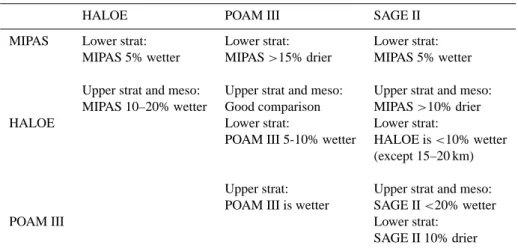
MIPAS (Fischer and Oelhaf, 1996) is a Michelson Interfer-ometer launched aboard ENVISAT in March 2002. By pas-sively sounding the atmosphere in the near infrared, verti-cal profiles of trace gases such as water vapour can be de-termined. MIPAS humidity profiles are available from 12– 60 km. The estimated error standard deviation for v4.61 is 10–20% near the tropopause, 3–10% in the 15–40 km layer, and 3–15% in the 40–60 km layer; the total error (random plus systematic, i.e. bias) is 20–25% near the tropopause, 15–20% in the 15–40 km layer, and 20–50% in the 40 km– 60 km layer (Raspollini et al., 2006). The main systematic errors are associated with spectroscopy and horizontal tem-perature errors. Comparison of the MIPAS humidity profiles with balloon and aircraft data (Oelhaf et al., 2004); ground-based radiometer and lidar data (Pappalardo et al., 2004); and HALOE, SAGE II and POAM III satellite data (Weber et al., 2004), shows good agreement between 15 km and 30 km. However, above 30 km the MIPAS retrievals have a positive bias of up to 20% compared to the satellite data and of 7–15% compared to ground-based radiometer and lidar data. Juckes (2007), when comparing MIPAS data to other satellite data, found that in general MIPAS data compared most favourably with HALOE data, with larger departures from the SAGE II and POAM III data sets. In the lower stratosphere MIPAS is marginally wetter (by 5%) than HALOE and SAGE II data, while MIPAS data is significantly drier than POAM III data (by more than 15%). In the upper stratosphere POAM III data compares most favourably with MIPAS data, while MI-PAS data is wetter than HALOE (10%) and drier than SAGE II (>10% at 1 hPa). Lahoz et al. (2006) also document the relatively poor quality of v4.61 MIPAS water vapour in the
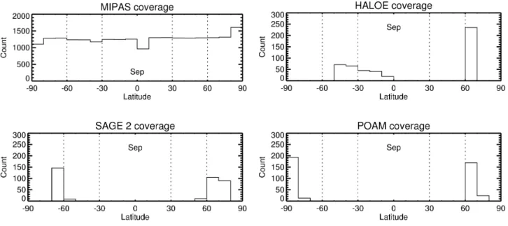
Fig. 1. Latitudinal coverage of MIPAS (top left), HALOE (top right), SAGE II (bottom left) and POAM III (bottom right) profiles over the
intercomparison period (29 August–29 September 2003). Data are collected in 10◦latitude bins.
southern winter upper stratosphere, where unrealistically wet values were found. In the UTLS region the MIPAS retrievals have a small negative bias compared to the balloon and air-craft data. The good spatial coverage of the MIPAS data is highlighted in Fig. 1, which shows that there are at least 900 profiles available in each 10◦latitude bin during September
2003.
3.2 HALOE
The Halogen Occultation Experiment (HALOE; Russell III et al., 1993) uses solar occultation to derive atmospheric con-stituent profiles. We use Version 19 HALOE data, which is available from the HALOE website (http://disc.sci.gsfc. nasa.gov/data/datapool/UARS/HALOE/). For water vapour there is a combined systematic and random uncertainty in the lower stratosphere of between 14% and 24%, and up to 30% in the upper stratosphere. The agreement with correla-tive measurements is typically better than 10% (Harries et al., 1996; Kley et al., 2000). The agreement with SAGE II wa-ter vapour measurements (version 6.2) is betwa-ter than 10% in the 15–40 km region (Taha et al., 2004), with the HALOE water vapour exceeding SAGE II everywhere except in the 15–20 km range. The solar occultation technique means that the vertical resolution of the retrievals is high, ∼2 km, but it also means that the data are sparse in time and space, with about 15 observations (for both sunrise and sunset) per day at each of two latitudes. During September 2003 HALOE data are only available between around 0◦N to 50◦S and 60– 70◦N (Fig. 1). Table 1 summarises the relative biases found between the different satellite instruments.
3.3 SAGE II
The Stratospheric Aerosol and Gas Experiment II (SAGE II) sensor was launched in 1984 and also uses solar occul-tation to derive atmospheric constituent profiles (Mauldin III et al., 1985). The vertical resolution of the measure-ments is ∼ 500 m. We use version 6.2 data (Thomason et al., 2004), which are available from http://www-sage2.larc.nasa. gov/index.html. In the 15–40 km altitude range, the com-bined random error for single profiles is between 10% and 20%. In addition, the measurement bias seen in previous retrieval versions has been almost totally eliminated in ver-sion 6.2 (Thomason et al., 2004). Up to 40 km, the SAGE II data agree within 10% with frost point hygrometer, HALOE, POAM III and ILAS (Improved Limb Atmospheric Spec-trometer) data, and within 15–20% with Mk IV interferome-ter data (Taha et al., 2004). In this range, the SAGE II values are less than those from POAM III at all levels and less than those from HALOE everywhere apart from below 20 km. Above 40 km, SAGE II water vapour profiles are often noisy and show an increasing positive bias (up to 20% compared to HALOE data). Around the hygropause, comparison with other satellite-borne instruments is often problematic, but comparison with balloon-borne instruments (frost point hy-grometer and the Mk IV interferometer) shows agreement to within 10% (Taha et al., 2004). Observational coverage for September 2003 is shown in Fig. 1.
3.4 POAM III
The Polar Ozone and Aerosol Measurement III (POAM III) sensor is a solar occultation instrument which flies on a
Table 1. A summary of water vapour biases between MIPAS, HALOE, POAM III and SAGE II instruments in the stratosphere and lower
mesosphere.
HALOE POAM III SAGE II
MIPAS Lower strat: Lower strat: Lower strat:
MIPAS 5% wetter MIPAS >15% drier MIPAS 5% wetter
Upper strat and meso: Upper strat and meso: Upper strat and meso: MIPAS 10–20% wetter Good comparison MIPAS >10% drier
HALOE Lower strat: Lower strat:
POAM III 5-10% wetter HALOE is <10% wetter (except 15–20 km)
Upper strat: Upper strat and meso: POAM III is wetter SAGE II <20% wetter
POAM III Lower strat:
SAGE II 10% drier
spacecraft with a polar, sun-synchronous orbit; it provides 14 solar occultation measurements per day around two cir-cles of latitude, one for each hemisphere. Northern hemi-sphere measurements are made at local sunset, and South-ern hemisphere measurements are made at local sunset from October to March and at local sunrise from April to Septem-ber (our period of interest). Because of the satellite orbit used, all the observations are at high latitudes. We use Ver-sion 4 data, which are available from http://wvms.nrl.navy. mil/POAM/poam.html. The vertical resolution of the humid-ity retrievals is 1 km in the lower stratosphere, rising to 3 km in the upper stratosphere. Lumpe et al. (2006) show that Ver-sion 4 retrievals have a preciVer-sion of 5–7% throughout the stratosphere. They are biased high compared to correlative observations in the lower and middle stratosphere. Compar-isons with HALOE and SAGE II data also indicate differ-ences between sunrise and sunset POAM III retrievals, with sunset retrievals larger than sunset retrievals by 5–10%. In the northern hemisphere, POAM III water vapour is around 5–10% high compared to all correlative observations in the 12–35 km range. At higher levels, around 40 km, POAM III values exceed HALOE values but are fairly similar to MIPAS values. Figure 1 also highlights the poor availability of ob-servational data for studying the humidity of the stratosphere prior to the launch of ENVISAT.
3.5 UARS climatology
To better understand how the different analyses compare with the independent data, the comparison is normalised by the UARS humidity field. This process is explained in Sect. 4. UARS water vapour profiles were taken from the UARS Reference Atmosphere Project website (http://code916.gsfc. nasa.gov/Public/Analysis/UARS/urap/home.html). The data selected are the extended HALOE/MLS dataset, which gives humidity profiles up to 0.1 hPa, in the form of zonal monthly
mean fields. A water vapour climatology field was created on the intercomparison grid (described in Sect. 4), for ev-ery 6-h period over the intercomparison. This was done by linearly interpolating the monthly mean files in time, by as-suming the UARS monthly mean files represent the 15th of every month. The UARS monthly mean fields are only avail-able up to 80 degrees north/south in the stratosphere and to 65 degrees north/south in the mesosphere. MIPAS and the independent data are available at higher latitudes and sequently the climatology was extended horizontally at con-stant value. Although this assumption may modify the rela-tive biases, it was felt justified to enable the higher latitudes to be analysed.
4 Method
As in the ozone intercomparison described by Geer et al. (2006), the humidity analyses have been interpolated onto the same common grid, prior to interpolation to observation locations for comparison. The common grid is 3.75◦ longi-tude by 2.5◦latitude, with 19 pressure levels. The pressure levels are those used in the UARS project, with 6 pressure levels per decade between 0.1–100 hPa. In the vertical, inter-polations were done linearly in the natural logarithm of the pressure. Horizontally, the interpolation is bi-linear in both longitude and latitude. Analyses are available every 6-h for comparison with observations. There is therefore a maxi-mum of a 3-h time difference between compared observation profiles and analyses.
The observations are interpolated onto the common grid vertical levels to ease comparison, as the different observa-tions have different vertical resoluobserva-tions. The observaobserva-tions that are used in the intercomparison have been quality con-trolled. For each profile, at each level, the observation must not be greater than the UARS climatology by more than
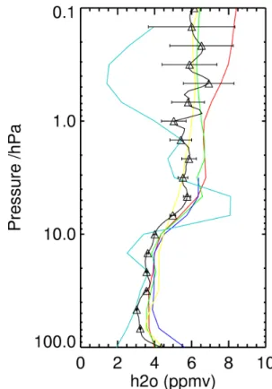
120%, otherwise it is flagged as missing. This has the impact of removing the observation profiles which are significantly different from the climatology, effectively removing outliers. None of the HALOE profiles were removed by this process, however 2%, 8% and 12% of MIPAS, SAGE II and POAM III profiles were removed respectively. The UARS clima-tology was made up of HALOE and MLS observations and therefore explains the good agreement between the HALOE data and the climatology. The removal of the other outly-ing observational profiles avoids poor data skewoutly-ing the bi-ases. For example, prior to the data consistency check, the extra SAGE II data produced very large biases in the south-ern hemisphere mid latitude lower stratosphere. The loss of data due to the quality control procedure is sufficiently small to avoid any significant loss of data coverage. Sensitivity tests completed by Geer et al. (2006) for the ozone compari-son (this uses a 12 hourly temporal resolution) show the cho-sen temporal and spatial resolution of the common grid has little impact on the mean differences between ozone observa-tions and analyses for levels below 0.5 hPa. Above 0.5 hPa, the processes that govern the ozone distribution have a time-scale shorter than 12 h. For example, in regions of rapid transport such as the polar vortex, or within the slow ascent of the tropics, the grid resolution had little impact on the mean differences. In the mid-latitude UTLS, the temporal resolu-tion was found to be more important and therefore the com-parison was completed every 6 h. Like ozone in the lower and middle stratosphere, water vapour can be considered a tracer species in the stratosphere and lower mesosphere, because the oxidation of methane or the photolysis of water vapour represents small terms in the water vapour budget compared to the transport term. Furthermore, the processes that govern the water vapour distribution have a time-scale longer than the temporal resolution of the common grid. Therefore, the grid chosen for the water vapour analysis is not expected to strongly influence the differences found between the water vapour observations and the analyses. Figure 2 illustrates that the common grid is capable of capturing most of the ver-tical variability in specific humidity in the upper stratosphere and lower mesosphere seen in the HALOE profile.
Figure 2 also highlights where particular analyses have problems assimilating the MIPAS profiles. The large dry bias in the mesosphere and the wet bias in the upper strato-sphere of the Met Office analyses can clearly be seen. Due to the poor performance of the Met Office humidity assim-ilation scheme, its results are not presented along side the other analyses but rather discussed in Sect. 6. The increas-ing ECMWF wet bias with altitude in the lower mesosphere is due to an incorrect use of the MIPAS observations above the model top, inflicting a wet bias in the specific humidity field down to about 0.5 hPa. Some MIPAS partial columns were partially above the top of the ECMWF model, and for the part above the model top, the model humidity was erro-neously taken to be zero. Such data should have been ex-cluded in the ECMWF analyses. In the following, we will
Fig. 2. Comparison of a HALOE profile at a resolution of 30 points
per decade (black line), HALOE values (black triangles) and er-ror bars on common grid levels with the four analyses, ECMWF (Red), BASCOE (Green), MIMOSA (Dark Blue) and the Met Of-fice (Light Blue), and the UARS climatology (Yellow) on 2 Septem-ber 2003 at 04:19, 6.45◦E, 65.73◦N.
therefore discard the ECMWF analyses above 0.5 hPa. This limit was chosen on the basis of departure statistics for MI-PAS retrievals and background error correlations.
Like the analysis fields, the UARS climatology is firstly interpolated onto the common grid and secondly to observa-tion locaobserva-tions, to enable the relative difference in the biases with height to be seen. At each observation profile location and common grid level, the difference in specific humidity between the observation and the different analyses is calcu-lated and then normalised by the corresponding UARS cli-matological value, as in Geer et al. (2006, Sect. 4). The av-erage normalised difference per level and per latitude bin is then calculated. Percentage differences are calculated for five latitude bands for ease of comparison; the high latitudes (90– 60◦) and the mid latitudes (60–30◦) in both hemispheres, and
the tropics (30◦S–30◦N). The intercomparison period runs
from 29 August 2003 to 29 September 2003. All the experi-ments commenced at least 10 days prior to the start of the in-tercomparison period (18 August, 15 August, July 2002 and 4 August for the ECMWF, MIMOSA, BASCOE and Met Of-fice analyses, respectively). The intercomparison period was chosen such that any spin up issues were resolved prior to the start of the intercomparison period.
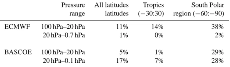
Table 2. The percentage of MIPAS observations rejected by each observational quality control system. No quality control has been applied
in the MIMOSA system, consequently all MIPAS retrievals have been assimilated. Higher rejection rates occur for the Tropics and the South Polar region for at least one system, so these regions are shown separately. For other regions rejection rates are low, typically well below 10%.
Pressure All latitudes Tropics South Polar range latitudes (−30:30) region (−60:−90)
ECMWF 100 hPa–20 hPa 11% 14% 38%
20 hPa–0.7 hPa 1% 0% 2%
BASCOE 100 hPa–20 hPa 5% 1% 29%
20 hPa–0.1 hPa 17% 7% 28%
5 Results
5.1 September monthly mean 12:00 UT analysis
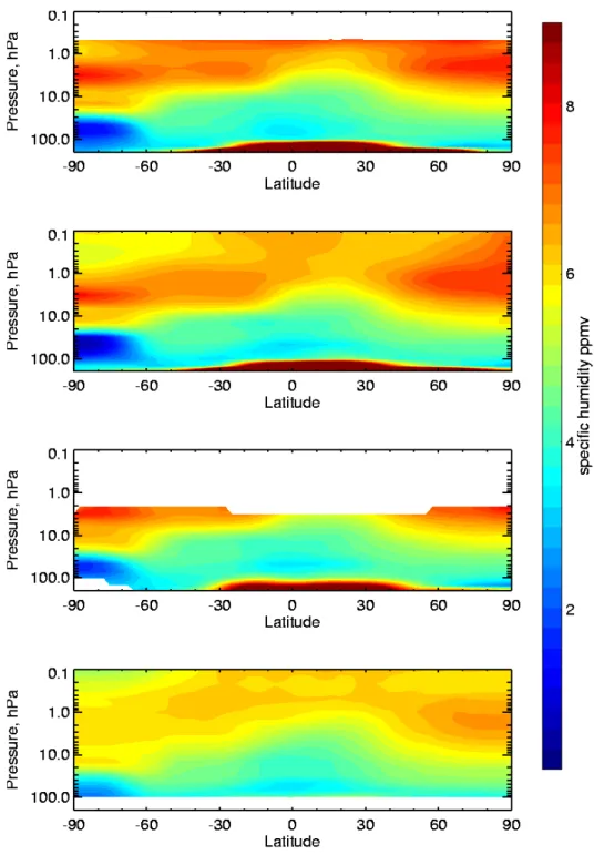
Figure 3 shows the monthly mean zonal water vapour anal-yses for the intercomparison period for the ECMWF, BAS-COE and MIMOSA systems. The UARS climatology water vapour field is also included. A number of well-known fea-tures can be seen in the stratospheric analyses and climatol-ogy. These include the very dry tropical tropopause region (near 100 hPa) and the dehydration within the Antarctic win-ter polar vortex (between 100–50 hPa Kley et al., 2000). The presence of a layer of dry (∼3 ppmv – parts per million by volume) air around the 100–200 hPa suggests that some of the air coming into the stratosphere in the tropics may be being transported rapidly polewards. This is in agreement with previous observational studies (e.g. Jackson et al, 1998). There is also an indication of slow upward transport of dry air at low latitudes via the Brewer-Dobson circulation. As the air is transported upwards, methane oxidation leads to an increase in humidity, which is reflected in the relatively moist air seen in the upper stratosphere and lower meso-sphere (levels above 10 hPa). Near the stratopause (near 1 hPa) the water vapour patterns are consistent with overturn-ing of the stratospheric air related to a change in the pattern of the Brewer-Dobson circulation. This change implies the replacement of upward low latitude transport by poleward transport and associated downward transport at high latitudes of moist air from the upper stratosphere / lower mesosphere to lower levels. This pattern is most apparent in the winter high latitudes, where downward transport is stronger.
The regions of the middle atmosphere where the specific humidity analyses differ from one another can be divided into the tropical water vapour minimum, the UTLS, the south-ern hemisphere polar vortex and the upper stratosphere and lower mesosphere (USLM). In the tropical UTLS, the shape and depth of the water vapour minimum differs from one analysis to another. The strength and extent of the south-ern hemisphere polar vortex also varies between the analyses, with MIMOSA appearing to have the smallest extent, while BASCOE has the largest and driest vortex. Between 1 hPa
and 10 hPa, the moist centres associated with the descend-ing arm of the Brewer-Dobson circulation vary in magnitude between the analyses, where BASCOE appears marginally drier. Above 1 hPa, the ECMWF analysis is considerably wetter at all latitudes than BASCOE.
When comparing the analyses to the UARS climatology, the features of the specific humidity fields are similar, al-though the climatology is generally less extreme, with a wet-ter UTLS and a drier USLM. As explained in Sect. 3 the MIPAS data assimilated in the analyses have a dry bias in the UTLS and wet bias in the USLM compared to most observa-tion types and this therefore may explain these differences.
5.2 Comparison with MIPAS and independent data
In this section, the ECMWF, BASCOE and MIMOSA anal-yses are compared with MIPAS data and with independent data from HALOE, SAGE II and POAM III. The compari-son with MIPAS data is a consistency check of the assimila-tion algorithms as this data has been assimilated to produce the analyses. The comparison with the other non-assimilated data is an independent evaluation of the quality of the resul-tant analyses. The discussion is focused on the mean dif-ferences between the analyses and these data, and the stan-dard deviation of this difference in the five different lati-tudinal bands. Each section of the middle atmosphere is taken in turn, starting with the UTLS, followed by the upper stratosphere, finishing with the lower mesosphere. Rejection statistics for the MIPAS retrievals for the different assimila-tion systems are summarised in Table 2. For the ECMWF and the BASCOE system, observations are rejected from the assimilation if they deviate too much from the model back-ground field, in order to remove outliers. No such quality control is included by MIMOSA. Higher rejection rates oc-cur over the South Polar region and the Tropics for at least one assimilation system, and these regions are shown sepa-rately in Table 2. Elsewhere, rejections are typically less than 10%, suggesting few outliers in the MIPAS retrievals. Higher rejections can reflect problems with the model background or the observations, or may result from stricter quality control.
Fig. 3. Monthly zonal mean specific humidity (ppmv) analyses for the intercomparison period for ECMWF (top), BASCOE (upper middle)
and MIMOSA (lower middle) and UARS climatology (bottom). MIPAS water vapour profiles have been assimilated in all cases except the UARS Climatology.
5.2.1 Upper troposphere lower stratosphere
The distinctive water vapour features of the UTLS region can be seen in Fig. 3, including the tropical (∼50–70 hPa, 30◦S–30◦N) and the southern hemisphere high latitude wa-ter vapour minima. As described by Kley et al. (2000), the tropical water vapour minimum is generated around Febru-ary, when the coldest tropopause temperatures have
dehy-drated the rising air. The vertical transport of the Brewer-Dobson circulation in the lower latitudes, has lifted this dry air to the position seen in Fig. 3. This feature is described in detail in Mote et al. (1996) and it is referred to as the “trop-ical tape-recorder”. The southern hemisphere water vapour minimum is associated with the cold interior of the polar vor-tex.
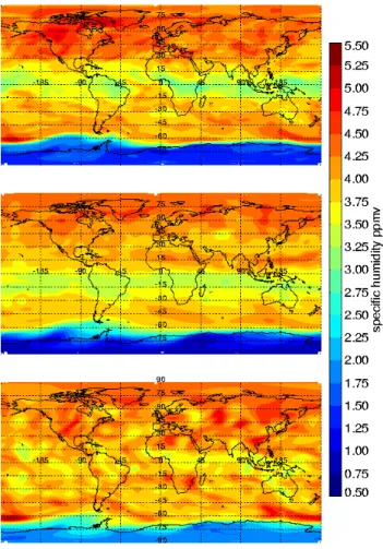
Fig. 4. Specific humidity field (ppmv) at 68 hPa on the 21
Septem-ber 2003 12:00 UT, for ECMWF (top), BASCOE (middle) and MI-MOSA (bottom).
The tropical water vapour minimum
The coverage and depth of the tropical water vapour min-imum in Fig. 3 can be seen to vary between the different analyses. Figure 4 shows how the specific humidity field varies as a function of latitude and longitude at 12:00 UT on 21 September 2003 around the water vapour minimum (68 hPa) in the three analyses. MIMOSA can be seen to have the wettest tropical water vapour minimum and ECMWF the driest. MIMOSA has assimilated the MIPAS observations most successfully in the tropics, as the bias with respect to the observations is almost zero at 68 hPa (Fig. 5). This is as expected, because the assimilation parameters are tuned to minimise the root mean square of the observation minus fore-cast vector. ECMWF and BASCOE have a small dry bias in comparison with the MIPAS observations of up to 5% in this region. The standard deviations of the analysis departures are approximately 15% for all three analyses (Fig. 6). Near the tropical tropopause (100 hPa) the dry biases of ECMWF and BASCOE increase to 20% and can be seen to occur at most latitudes in the UTLS. The standard deviations increase
to 30% at 100 hPa in the tropics and range between 10% and 40% across the different latitudes. The tropospheric set-up of the water vapour in the BASCOE analyses (see Sect. 2.2) ex-plains the close agreement between BASCOE and ECMWF systems in the UTLS. However, the quality control system in ECMWF rejects a much higher percentage of MIPAS ob-servations in the tropical lower stratosphere (14%) compared to BASCOE (1%), suggesting the ECMWF scheme may be more strict in this region.
HALOE data are the only independent data set in the trop-ical UTLS available to assess the realism of the different wa-ter vapour minima in the analyses. Figure 5 shows that be-tween 50 hPa and 70 hPa BASCOE matches the HALOE ob-servations most closely, with ECMWF and MIMOSA having a wet bias of 10–20%. However nearer the tropopause the biases are more similar to those with the MIPAS data, with ECMWF and BASCOE having dry biases of 5% and 10% re-spectively. The standard deviations of the differences range between 10% and 15% for the different analyses. HALOE has been found by Juckes (2007) to have a 5% dry bias rel-ative to MIPAS data and therefore this partly explains the differences seen.
Southern hemisphere polar vortex
Another problematic region in the lower stratosphere for the assimilation of humidity observations is the southern hemi-sphere polar vortex. In this region the persistent strong zonal flow acts as a barrier to meridional flow. In the very cold po-lar winter, the air trapped within the vortex is cooled and this allows PSC generation, leading to removal of water vapour and very dry air. Figure 3 highlights the strong humidity gradient between the dry polar air and the wetter air at mid latitudes and higher altitudes.
Figures 5 and 6 highlight the ability of the different sys-tems to assimilate the MIPAS observations in the southern hemisphere lower stratosphere. MIMOSA again assimilates the MIPAS observations effectively with a dry bias and a standard deviation of less than 10% and 30%, respectively. ECMWF and BASCOE have larger dry biases of 20% and up to 60%, respectively, and standard deviations ranging be-tween 10% and 40%. The BASCOE dry bias and standard deviation peak at 30 hPa in the Southern Hemisphere high latitudes reaching 60% and 35%, respectively. This large bias is likely to relate to the chemistry scheme applied in the BAS-COE system and is discussed later in this section. Figure 7 shows a comparison of MIPAS observations and the anal-yses, in 10◦latitude bands in the southern hemisphere high latitudes. The dry BASCOE bias reduces from 70% at 30 hPa between 70–90◦S to 35% between 60–70◦S. Both ECMWF and BASCOE rejected a high percentage of MIPAS observa-tions in the lower stratosphere south polar region (38% and 29%, respectively) and most likely reflects the poor quality of either the MIPAS observations or the model analyses in
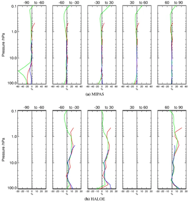
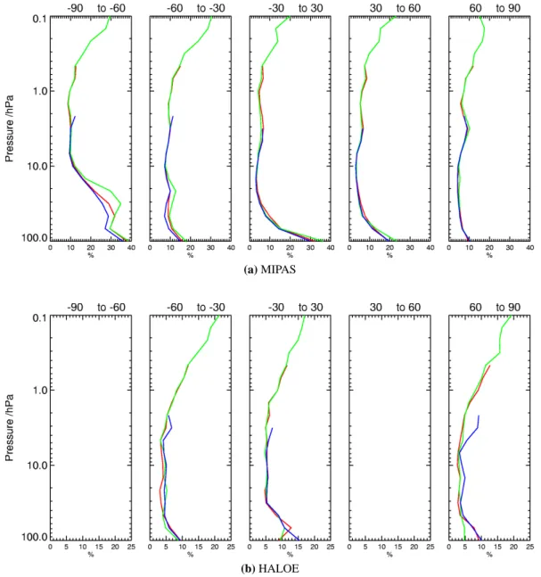
(a) MIPAS
(b) HALOE
Fig. 5. Mean of (Analysis–Observations) water vapour mixing ratio, normalised by climatology (in percent) over the intercomparison period,
for ECMWF (Red), BASCOE (Green) and MIMOSA (Blue), for the five different latitude bins. For rows (a) to (d), the analyses are compared with MIPAS, HALOE, SAGE II and POAM III data, respectively. If there are not any satellite profiles available, the graphs are blank.
this region. The large analysis – observation biases in this region suggest the latter maybe important.
With respect to independent data, the water vapour biases in the southern hemisphere high latitudes depend on the in-strument considered. Compared to POAM III data, the bi-ases seen for the different analyses are generally similar to MIPAS but slightly larger in magnitude. For example, the dry biases for all three analyses peak at 45 hPa with values of 80%, 50% and 40% (Fig. 5) for BASCOE, ECMWF and MI-MOSA respectively. The analysis departure standard devia-tions from POAM III observadevia-tions range between 10% and 60% from 10 hPa to 100 hPa for all three analyses. This ties in with the findings of Juckes (2007) that POAM III data is
15% wetter than MIPAS in the lower stratosphere. In com-parison with SAGE II data, BASCOE again has a dry bias up to 20% with a standard deviation of 10–20%, both peaking at 30 hPa. However, ECMWF and MIMOSA have a wet bias of 5% and 15% respectively and both have a standard deviation of 10–20%. The difference in the biases between the anal-yses and the SAGE II and POAM III data can be explained by: firstly SAGE II data has a dry bias relative to POAM III data (see Sect. 3); secondly, the SAGE II data is sampling the vortex boundary (60–70◦S), whereas POAM III samples the vortex core (>70◦S) and, as shown in Fig. 7, the analysis bias is generally less negative in the former region than in the latter.
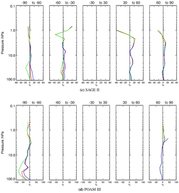
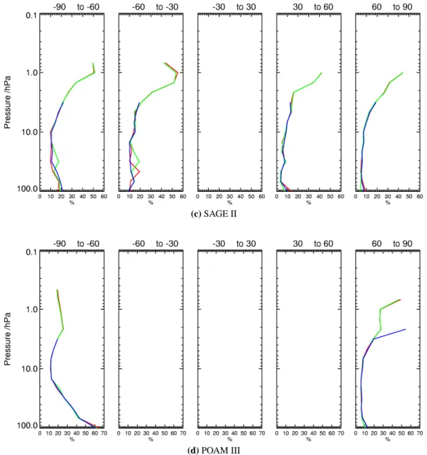
(c) SAGE II
(d) POAM III
Fig. 5. Continued.
To understand the cause of these biases, the analyses will be studied in more depth, concentrating on how the analyses represent the lower stratosphere vortex core moisture min-imum (70–90◦S), the latitudinal and vertical extent of this
moisture minimum and the transition to wetter mid latitude conditions.
In the analyses, the monthly mean average vortex mois-ture minimum occurs in the region 70–90◦S and between
150–30h Pa (Fig. 3). Figure 8 shows the specific humidity field over the southern hemisphere polar region, for each analysis and climatology, for one particular analysis time (12:00 UT, 21 September 2003) at a level within the mois-ture minimum (68 hPa). The stark contrast between the very dry polar air and the wetter mid latitude air is clearly seen in the zonally symmetric UARS climatology. The dryness
of the polar vortex varies between the different analyses, with BASCOE and ECMWF having a drier centre than MI-MOSA. Figure 9 shows an individual MIPAS profile on the 21 September 2003, located within the vortex core. In agree-ment with the latitudinal band averages seen in Fig. 7, MI-MOSA compares most favourably with the MIPAS profile between 100 hPa and 50 hPa. ECMWF and BASCOE both struggle to assimilate the profile and have dry biases of 20% and 40%, respectively, although ECMWF lies on the bounds of the observational error bars.
POAM III data are the only available independent data source within the vortex core. Figure 10 shows a compari-son between an individual POAM III profile and the different analyses. The uncertainty of the POAM profile within the po-lar vortex is highlighted by the very po-large observed error bars.
(a) MIPAS
(b) HALOE
Fig. 6. Standard deviation of (Analysis–Observations) water vapour mixing ratio, normalised by climatology (in percent) over the
intercom-parison period, for ECMWF (Red), BASCOE (Green) and MIMOSA (Blue), for the five different latitude bins. For rows (a) to (d), the observational data is MIPAS, HALOE, SAGE II and POAM III respectively. If there are not any satellite profiles available, the graphs are blank.
In agreement with the single MIPAS profile comparison, MI-MOSA is closest to the POAM III profile, while ECMWF and BASCOE have larger dry biases. The dry biases seen are larger than in comparison to the MIPAS profile and again tie in with the POAM III wet bias compared to MIPAS data.
Within the polar vortex, temperature mainly determines the specific humidity, due to the dehydrating impact of PSCs. The PSC sedimentation process is simulated in the BASCOE system, but not in the ECMWF and MIMOSA systems. It is therefore likely that the BASCOE dry bias in the south-ern hemisphere polar vortex relates to the PSC parametriza-tion, but also the observational quality control scheme.
Al-though the BASCOE PSC parametrization scheme can pro-duce a good ozone hole representation Geer et al. (2006), it is likely that the scheme overestimates water vapour loss by PSC sedimentation, producing very dry polar air. To im-prove the BASCOE analyses in this region, would require an improved PSC sedimentation scheme and a relaxation of the data filtering process.
Both the latitudinal and vertical extent of the southern hemisphere polar water vapour minimum will be studied next. Figure 3 highlights the latitudinal extent of this min-imum and how it varies between the different analyses. Al-though the total size of the region of dry polar air appears
(c) SAGE II
(d) POAM III
Fig. 6. Continued.
approximately constant between the different analyses, the very dry centre in the ECMWF and BASCOE analyses stretches further equatorward than for MIMOSA. For exam-ple, the water vapour content at 70◦S is wetter in MIMOSA monthly mean than in the other two analyses. Figures 4 and 8 also show for one day (12:00 UT, 21 September 2003) that the southern hemisphere polar vortex is smaller in the MI-MOSA analysis. By looking at the bias of the analyses with respect to MIPAS data in the 60–70◦band, the faithfulness of the polar vortex extent with respect to MIPAS data between the analyses can be inferred. Figure 7 shows that between 100 hPa and 50 hPa in this latitude band, the MIMOSA bias is negligible, whereas ECMWF and BASCOE have a 20– 30% dry bias. This suggests that the smaller extent of the
MIMOSA dry core in the southern hemisphere polar vortex is more consistent with the MIPAS data.
Figure 3 highlights the differences in the vertical extent of the dry region of the southern hemisphere polar vortex, be-tween the different analyses. Over the intercomparison pe-riod, the BASCOE moisture minimum has a greater vertical extent, reaching approximately 20 hPa, while for ECMWF and MIMOSA it only reaches approximately 30 hPa. Fig-ure 11 describes how the specific humidity field varies over the South Pole at 12:00 UT on the 21 September 2003 at 32 hPa, which is in this region of the upper limit of the dry vortex region. At this level, the BASCOE specific humidity values are less than 1.5 ppmv in contrast to the 3 ppmv seen in MIMOSA and ECMWF. Dehydration over the vortex core,
Fig. 7. Mean of (Analysis-MIPAS), normalised by climatology (in percent) over the intercomparison period, for ECMWF (Red), BASCOE
(Green) and MIMOSA (Blue), concentrating on the southern high latitudes (50◦S to 90◦S in 10◦bands).
Fig. 8. Polar stereographic projection of the specific humidity field (ppmv) for the southern hemisphere on 21 September 2003 12:00 UT at
Fig. 9. A comparison of a MIPAS profile (black, with one
stan-dard deviation error bars – 21 September 2003, 10:13 a.m., 168◦W, 74◦S) with the different analyses and climatology (colours as Fig. 2).
associated with the cold polar temperatures, limits the pres-ence of the descended moist upper stratospheric air to the outer rim of the vortex in the ECMWF and MIMOSA anal-yses. A comparison with MIPAS observations indicates that at approximately 30 hPa, the BASCOE analyses are too dry, with a bias of 70% (Fig. 7). A comparison with a single MI-PAS profile (Fig. 9) shows that the gradient of increasing hu-midity with altitude in the BASCOE analysis between 40 hPa and 10 hPa is too steep and is displaced vertically upwards by approximately 10 hPa. This gradient in the MIMOSA and ECMWF analyses is also too steep, however the gradient is better located in the vertical.
As described previously, the peak in the biases with re-spect to independent observations in the southern hemisphere high latitudes occurs at 30–45 hPa. A comparison with a single POAM III profile (Fig. 10) also highlights the prob-lematic transition zone above the vortex. In the BASCOE analysis, PSC sedimentation can still be seen to be very im-portant at 32 hPa (producing the very low humidity values), whereas according to the POAM and MIPAS data this may not be the case. As explained earlier, the BASCOE PSC sed-imentation scheme appears to be overestimating the water vapour loss. This BASCOE dry bias may be further exac-erbated by the low sulphate aerosol loading in 2003 (due to
the last major volcanic eruption occurring in 1991), which would not have been captured in the BASCOE model. Sul-phate aerosols are responsible for generating ice particles and consequently water vapour sedimentation (via NAT particles, Daerden et al., 2007), reduced aerosol loading therefore re-sults in reduced drying. BASCOE is the only model to in-clude a PSC parametrization and the results presented here highlight the complexity of attempting chemical assimilation with explicit chemistry models in comparison to tracer trans-port models. The peak in the biases at 30–45 hPa in all three analyses therefore relate to the inability of the analyses to correctly capture the strong vertical humidity gradient above the southern hemisphere polar vortex.
5.2.2 Upper stratosphere and lower mesosphere
In the upper stratosphere (here used to refer to 20–1 hPa) there are two processes which affect the water vapour con-centration and distribution, the production of water vapour by methane oxidation and the horizontal and vertical transport by the Brewer-Dobson circulation. Figures 5 and 6 show that the analyses compare very favourably with the MIPAS obser-vations at these levels, with biases less than 5% and standard deviations less than 10%, indicating the observations have been well assimilated. A comparison with independent data however shows that around 2–3 hPa there is often a wet bias. This is particularly true with respect to HALOE data, where the analyses have a 20% wet bias over most of the upper stratosphere, peaking at 2hPa. This contradiction may in part relate to the MIPAS wet bias relative to the HALOE data de-scribed in Sect. 3. However at selected latitudes, wet biases at this altitude also exist with respect to POAM III and SAGE II data, with peaks in the standard deviations of the analysis departures, and therefore the source of this bias deserves fur-ther investigation.
Figure 3 highlights that at the 2–3 hPa the water vapour field is dominated by a strong latitudinal gradient. At higher latitudes, moist older air is found, which has descended from the upper stratosphere where longer exposure to methane oxidation has given the air a relatively wet signature. The younger, dry, low latitude air has risen from the lower strato-sphere. The bias peaks are therefore highly likely to relate to the ability of the different analyses to represent this strong latitudinal gradient in water vapour. In the monthly mean water vapour analyses (Fig. 3) and through consideration of daily plots (not shown), BASCOE has a weaker northern hemisphere moist centre at 2 hPa. BASCOE is also found to have a slightly smaller wet bias when compared to HALOE and POAM III data in this region than ECMWF and therefore appears the more realistic representation. A similar feature is also found in the southern hemisphere mid latitudes. It is not possible to assess which of the southern hemisphere high latitude analyses are most realistic as the data comparisons vary greatly. MIMOSA has a very noisy daily water vapour field at 2 hPa, leading to a variety of biases and standard
deviations. The patchy nature of the MIMOSA analyses will be discussed in Sect. 5.2.3. Between 1–2 hPa at most lati-tudes, there is a large dry bias of the analyses with respect to the SAGE II data, that is not seen when compared to the other observations. As discussed in Sect. 3, the SAGE II data is found to be noisy in this region and gives wetter readings than the other satellite data. The poor quality of the SAGE II data in this region is therefore likely to be responsible for the large biases seen.
In the lower mesosphere (pressures lower than 1 hPa), BASCOE and ECMWF analyses compare well with the as-similated MIPAS data, with biases of less than 10%. Above 0.2 hPa, BASCOE has an increasing wet bias and standard deviation of analysis departures, however the proximity to the model top is expected to degrade the quality of the anal-yses. In comparison to independent data, the analyses are again reasonable with biases and standard deviations of less than 20% and 25% respectively. A higher percentage of MI-PAS observations were rejected in the USLM by the BAS-COE system compared to ECMWF (Table 2). This is es-pecially true in the southern hemisphere high latitudes and again may indicate the poor quality of the observations or analyses near the model top.
5.2.3 Spatial structure of the analyses
Figures 4, 8 and 11 give a feel for the spatial coherence of the specific humidity fields generated by the different data assimilation schemes. These figures highlight that al-though the different analyses show similar large-scale wa-ter vapour features, there are considerable variations at the smaller scale; for example MIMOSA has a noisier water vapour field throughout the depth of the stratosphere. Dif-ferences in the assimilation schemes, grid resolutions and observation filtering criteria are likely responsible for these differences. The tracer like properties of water vapour in the stratosphere and lower mesosphere make the spatial variabil-ity in the MIMOSA analyses unrealistic. Unlike ECMWF and BASCOE, MIMOSA did not filter out any of the MIPAS observations and therefore, the poor quality of some of the profiles would pass through to the analyses. Another reason for the unrealistically noisy MIMOSA water vapour fields is likely due to the error correlations being related to PV. The PV field can be quite variable in space, especially in the mid latitudes. Even if a grid point that is relatively far from a MI-PAS observation has a similar PV value as found at the obser-vation location, it will be given a similar water vapour incre-ment. The patchy structure of the analyses may also there-fore reflect the patchy nature of the PV field. Consequently, although the MIMOSA analyses compare most favourably with the MIPAS observations, the smoother ECMWF and BASCOE stratospheric water vapour fields are closer to what one might expect from a water vapour field that is determined mainly by the large scale circulation, photochemistry and lo-cation specific dehydration (Kley et al., 2000). Further
ob-Fig. 10. A comparison of a POAM profile (black, with one
stan-dard deviation error bars – 21 September 2003, 12:00 p.m., 283◦E, 88◦S) with the different analyses and climatology (colours as Fig. 2).
servations of the daily stratospheric water vapour field and detailed analysis of the MIPAS observations and MIMOSA analysis increments would be required to assess whether any part of the variability seen in the MIMOSA analyses has a physical justification. The BASCOE water vapour fields are particularly smooth and reflect its low horizontal grid resolu-tion compared to the resoluresolu-tion of the MIPAS observaresolu-tions.
6 Met Office analyses
The Met Office also assimilated MIPAS water vapour pro-files into their system over the intercomparison period, but these analyses have not been included in the intercompari-son described in Sect. 5 due to their poor performance. We illustrate this here using analysis minus MIPAS percentage differences, and the standard deviation of this difference, for all latitudes (Fig. 12). The poor quality of the Met Office analyses compared to the others is very clear. At nearly all pressure levels, the Met Office analyses have a large dry bias compared to the MIPAS observations. In the lower strato-sphere there is a dry bias of 20–40% and in the USLM, the dry bias increases with altitude, with the largest bias exceed-ing 50%. The standard deviation of analysis departures is
Fig. 11. Polar stereographic projection of the specific humidity field (ppmv) for the southern hemisphere on the 21 September 2003 12:00 UT
at 32 hPa, for ECMWF (top left), BASCOE (top right), MIMOSA (bottom left) and climatology (bottom right).
Fig. 12. Top: mean of (Analysis - MIPAS) water vapour mixing
ratio, normalised by climatology (in percent) over the intercom-parison period, for ECMWF (Red), BASCOE (Green), MIMOSA (Blue) and Met Office (light Blue), for all latitudes. Bottom: as top but standard deviation rather than mean difference.
particularly large in the upper stratosphere, where it exceeds 50%. These biases occur at all latitudes, but are worst in the high latitudes (not shown). Over the intercomparison period, only approximately 4% of MIPAS observations in the lower stratosphere were rejected by the Met Office quality control scheme. However, in the USLM 37% of MIPAS observa-tions were rejected, a much higher quantity than rejected by the other models, reflecting the model’s poor background hu-midity field.
The Met Office assimilation system used in these experi-ments is as described in (Geer et al., 2006), but with a num-ber of improvements to the forecast model. The model has 50 vertical levels ranging from the surface to ∼0.1 hPa and a horizontal resolution of 3.75◦longitude by 2.5◦latitude. The model dynamical equations, including the transport scheme, have a semi-Lagrangian formulation (Davies et al., 2005), and the model also includes a parametrization of the produc-tion and loss of water vapour in the USLM by methane ox-idation and photolysis. The data assimilation uses 3D-Var (Lorenc et al., 2002) with a 6-h assimilation window. The humidity control variable used is normalised specific humid-ity, as described by H´olm et al. (2002), and similar to that used by ECMWF. In addition, any correlation between tem-perature and specific humidity is removed from the control variable, following Dee and da Silva (2003). In these ex-periments the analysed specific humidity field is limited to between 0 ppmv and 12 ppmv, in order to ensure the continu-ity of the run. Without this pre-imposed limit, after a couple of weeks of assimilation, due to unrealistically large humid-ity analysis increments, the stratospheric water vapour field reached significantly higher values and resulted in the failure
of the run. The limit of 12 ppmv was chosen to ensure that the experiment ran without failure but also to allow plenty of scope for more realistic humidity analysis increments to be retained by the system.
The Met Office bias with respect to the MIPAS observa-tions shown in Fig. 12 can be seen after one 6-h assimila-tion window, when starting from a realistic background. It is therefore clear that these biases relate directly to the assim-ilation scheme and its resultant humidity increments, rather than the model dynamics or parametrizations. Many of the problems associated with the humidity assimilation may be linked to the specification of the background error covari-ances.
The background error covariances for the new humidity control variable were generated using the National Meteo-rological Centre (NMC) method (Parrish and Derber, 1992). In this method, model errors are assumed to be represented by the difference between forecasts of different length. The NMC error covariances used here were based on differences between a series of 24 and 48-h forecasts. These forecasts were generated from operational Met Office analyses. Such analyses do not include MIPAS observations and the resul-tant lack of water vapour observations in the stratosphere means that there is considerable doubt as to whether the NMC method can produce realistic error variances and ver-tical correlations for stratospheric water vapour. Support for this assertion comes from (Polavarapu et al., 2005a), who showed that use of NMC temperature covariances led to the production of unphysical temperature analyses above 1 hPa, where there are no temperature observations available to con-strain the analyses.
Investigations into the characteristics of the NMC humid-ity covariances found that the error variances, at a partic-ular level, often exceeded the background humidity value, and that the vertical correlations were unrealistically deep. For example, correlations were found between the boundary layer and the mesosphere, which means that a bias in the tro-posphere could therefore erroneously give rise to a bias in the mesosphere. Tools were developed at the Met Office to cut back both the error correlations and variances and tested us-ing sus-ingle observation experiments. Background error vari-ances were cut down to 50% of their background humidity value, while vertical correlations deeper than 8 km were sup-pressed. The scaling tools were found to have some positive impact, removing many large inappropriate stratospheric hu-midity increments. The scaling tools could not however im-prove upon the profile signature seen in Fig. 12. Even af-ter scaling of the covariance matrix, smaller scale, erroneous humidity increments were still added at every assimilation cycle.
An explanation for the persistence of these erroneous in-crements, even after scaling, is as follows. In the Met Office assimilation scheme, the background error covariance matrix is mathematically transformed prior to use, in order to re-move all non-zero off-diagonal terms. Without such a
trans-form, inversion of the background error covariance matrix would be computationally impossible. In the vertical, the er-ror covariance matrix is transformed into orthogonal vertical modes, such that the errors are uncorrelated between modes. The vertical correlation scaling mentioned above is applied before the vertical mode calculation. However, if the vertical error correlations are reduced excessively, or non-smoothly with height, it is found that the vertical mode calculation can introduce other, probably spurious, deep vertical correla-tions. If weaker scaling is applied, spurious correlations are not introduced by the vertical mode calculation, but the scal-ing is too weak to adequately remove the strong, erroneous vertical correlations present in the original covariances cal-culated by the NMC method. Single observation tests show that, for a whole range of vertical correlation scalings used, the scaling approach proves unsuccessful in removing the er-roneous deep correlations between the tropopause and the mesosphere.
A possible way forward is to reconsider the way in which the humidity background error covariance matrix is calcu-lated, rather than to scale existing covariances, as we have attempted here. A recent study by Jackson et al. (2008), has shown that the 3D-Var analyses on which the NMC covari-ance calculation was based, suffer from a lack of dynamical balance between the mass and wind fields. Spurious grav-ity waves are generated to restore this balance and can be seen in a 24-h forecast and consequently are present in the NMC error covariance matrix. This may explain the unreal-istic vertical correlations in the humidity covariance matrix reported here. Of course, the presence of a spurious gravity wave signal in the error covariances may have an adverse ef-fect on all analysis variables, but this efef-fect may be greatest for humidity because of the lack of suitable stratospheric hu-midity observations to constrain the analyses on which the NMC method is based.
Solutions to this problem include the use of better-balanced analyses in the NMC calculation. For example, at the Met Office, 3D-Var analyses have recently been su-perseded by 4D-Var analyses, which are in much better dy-namical balance and give rise to NMC covariances which contain a reduced spurious gravity wave signal. Other tech-niques of calculating error covariances may also be more effective at removing spurious gravity waves. Such tech-niques include the method described by Polavarapu et al. (2005b) (the so-called Canadian Quick covariances) and the use of ensembles. Ensembles are used to calculate back-ground error covariances at ECMWF. This may explain why the ECMWF stratospheric humidity analyses presented here are much more accurate than the corresponding Met Office analyses, even though the humidity control variable used at both institutes is very similar. It is not easy to apply the ECMWF covariances to the Met Office DA scheme, due to the different model formulations, however the use of ensem-bles to generate covariances is being further developed at the Met Office.