HAL Id: hal-00286238
https://hal.archives-ouvertes.fr/hal-00286238
Submitted on 9 Jun 2008
HAL is a multi-disciplinary open access
archive for the deposit and dissemination of
sci-entific research documents, whether they are
pub-lished or not. The documents may come from
teaching and research institutions in France or
abroad, or from public or private research centers.
L’archive ouverte pluridisciplinaire HAL, est
destinée au dépôt et à la diffusion de documents
scientifiques de niveau recherche, publiés ou non,
émanant des établissements d’enseignement et de
recherche français ou étrangers, des laboratoires
publics ou privés.
Evolution of massive protostars: the IRAS 18151-1208
region
M. Marseille, Sylvain Bontemps, Fabrice Herpin, F. F. S. van der Tak, C. R.
Purcell
To cite this version:
M. Marseille, Sylvain Bontemps, Fabrice Herpin, F. F. S. van der Tak, C. R. Purcell. Evolution of
massive protostars: the IRAS 18151-1208 region. Astronomy and Astrophysics - A&A, EDP Sciences,
2008, 488, pp.579-595. �10.1051/0004-6361:200809798�. �hal-00286238�
! ESO 2008 May 29, 2008
Evolution of massive protostars: the IRAS 18151
−
1208 region
!
M. Marseille
1,2, S. Bontemps
1,2, F. Herpin
1,2, F. F. S. van der Tak
3, and C. R. Purcell
41 Universit´e Bordeaux 1, Laboratoire d’Astrophysique de Bordeaux email: [marseille;bontemps;herpin]@obs.u-bordeaux1.fr 2 CNRS/INSU, UMR 5804, BP 89, 33270 FLOIRAC, France.
3 SRON Netherlands Institute for Space Research, Landleven 12, 9747 AD Groningen, The Netherlands. email: [email protected]
4 University of Manchester, Jodrell Bank Observatory, Macclesfield, Cheshire SK11 9DL, United Kingdom email: [email protected]
29 May 2008
ABSTRACT
Context.The study of physical and chemical properties of massive protostars is critical to better understand the evolutionary sequence which leads to the formation of high-mass stars.
Aims.IRAS 18151−1208 is a nearby massive region (d = 3 kpc, L ∼ 2×10⁴ L
%) which splits into three cores: MM1, MM2 and MM3 (separated by 1&–2&). We aim at (1) studying the physical and chemical properties of the individual MM1, MM2 and MM3 cores; (2) deriving their evolutionary stages; (3) using these results to improve our view of the evolutionary sequence of massive cores.
Methods.The region was observed in the CS, C34S, H2CO, HCO+, H13CO+, and N2H+lines at mm wavelengths with the IRAM 30m and Mopra telescopes. We use 1D and 2D modeling of the dust continuum to derive the density and temperature distributions, which are then used in the RATRAN code to model the lines and constrain the abundances of the observed species.
Results.All the lines were detected in MM1 and MM2. MM3 shows weaker emission, or even is undetected in HCO+and all isotopic species. MM2 is driving a newly discovered CO outflow and hosts a mid-IR-quiet massive protostar. The abundance of CS is significantly larger in MM1 than in MM2, but smaller than in a reference massive protostar such as AFGL 2591. In contrast the N2H+abundance decreases from MM2 to MM1, and is larger than in AFGL 2591.
Conclusions.Both MM1 and MM2 host an early phase massive protostar, but MM2 (and mid-IR-quiet sources in general) is younger and more dominated by the host protostar than MM1 (mid-IR-bright). The MM3 core is probably in a pre-stellar phase. We find that the N2H+/C34S ratio varies systematically with age in the massive protostars for which the data are available. It can be used to identify young massive protostars.
Key words.ISM: individual objects: IRAS 18151−1208 – ISM: abundances – Stars: formation – Line: profiles
1. Introduction
How high-mass stars form is still an open issue (e.g. Zinnecker & Yorke 2007). It is particularly not clear whether the for-mation process for OB/high-mass stars is different from the way solar-type/low-mass stars form. Stars more massive than ∼10 M% may form like a scaled-up version (high accretion
rates) of the single (or monolithic) collapse observed for the low-mass stars, or require a more complex process in which competitive accretion inside the central regions of a forming cluster may play a decisive role (e.g. Bonnell et al. 2004). In the first scenario, the observed high-mass clumps (100 to
Send offprint requests to: M. Marseille
! Observed with the IRAM 30m and Mopra telescopes. IRAM is supported by INSU/CNRS (France), MPG (Germany) and IGN (Spain). The Mopra telescope is part of the Australia Telescope which is funded by the Commonwealth of Australia for operation as a National Facility managed by CSIRO.
1000 M%; 0.5 pc in size) are expected to fragment to form
self-gravitating high-mass cores (10 to 100 M%; 0.01−0.1 pc in size;
e.g. Krumholz et al. 2007) which would collapse individually to form a massive single or binary stars. In the second scenario, the competitive accretion is expected to occur inside the high-mass clumps. The study of the properties of high-high-mass clumps is therefore a central observational issue to progress in our un-derstanding of the earliest phases of high-mass star formation.
From a selection of IRAS sources not associated with any bright radio source but having the IRAS colors of UC-HII
re-gions (as defined by Wood & Churchwell 1989), Sridharan et al. (2002) have built a sample of so-called High Mass Protostellar Objects (hereafter HMPOs) which would corre-spond to the pre-UC-HIIphase of the formation of high-mass
stars. Beuther et al. (2002b) found that the HMPOs were sys-tematically associated with massive clumps as detected in the dust continuum and in CS line emission. These clumps are good candidates to correspond to the earliest phases of
high-mass star formation. They have not yet formed any bright H regions and contain a large amount of gas at high densities. The precise evolutionary stages of the individual HMPOs might however be very diverse and they require to be derived indi-vidually through dedicated, detailed studies.
Recently, Motte et al. (2007) investigated the whole Cygnus X complex and obtained a first unbiased view of the evolutionary scheme for high-mass clumps and cores. Like for the HMPOs, the massive clumps (∼0.5 pc in size) in Cygnus X could be resolved into massive cores (∼0.1 pc). Roughly half of these cores were found to be very bright in the (mid)-infrared (such as AFGL 2591; e.g. van der Tak et al. 1999), and there-fore very luminous: the mid-IR high-luminosity massive cores. The other half are weak or not detected in the mid-IR, here-after the IR-quiet massive cores. Surprisingly all the mid-IR-quiet massive cores were however found to drive powerful SiO outflows. They could therefore be safely understood as the precursors of the infrared high-luminosity massive cores.
IRAS 18151−1208 is a rather typical (L ∼ 104L
%) and
rel-atively nearby (3 kpc) HMPO (Sridharan et al. 2002). Beuther et al. (2002b) show that the clump actually splits into four in-dividual cores MM1, MM2, MM3 and MM4 (see Fig. 1 for an overview of the region). In addition MM1 seems to further split into two cores, separated by 16&&. We hereafter refer to
MM1-SW for the secondary peak in the South-West of MM1 which possibly hosts an embedded protostar (Davis et al. 2004). The weakest core MM4 is clearly outside the main region, hence it will not be further considered in this paper. A CO outflow toward MM1 was discovered by Beuther et al. (2002c). The MM1 and MM2 cores have sizes roughly two times larger, and similar masses (using the same dust emissivity and tempera-ture) than the most massive cores in Motte et al. (2007). The IRAS source coincides with MM1 and no significant IRAS contribution can be safely attributed to MM2 or MM3. MM3 is the least massive and compact core and could actually be a still quiescent or pre-stellar core. The IRAS 18151−1208 region is therefore particularly interesting to study since it hosts three individual cores which could be interpreted as high-mass star formation sites in three different evolutionary stages. Millimeter and sub-millimeter wave observations are reported in McCutcheon et al. (1995) and Beuther et al. (2002b). The near-IR counterparts (H2 jets and HH objects) of the CO
out-flow driven by MM1 have been imaged by Davis et al. (2004). Molecular line observations compared with results of line modeling based on a physical model of the source is a classical technique to constrain physical and chemical properties of pro-tostellar objects (see Ceccarelli et al. 1996; van der Tak 2005, for a review). While different approaches can be adopted, the most reliable and most often used method consists in constrain-ing first the physical (density and temperature distributions) model from the dust continuum emission (mid-IR to millime-ter wavelengths), and then use this physical model to derive the fractional abundances of molecular species from line emission modeling (van der Tak et al. 1999; Hogerheijde & van der Tak 2000; Sch¨oier et al. 2002; Belloche et al. 2002; Hatchell & van der Tak 2003). Due to the dramatic changes in physical con-ditions inside the protostellar envelopes (increase of density and temperature, radiation, shocks) chemical evolution is
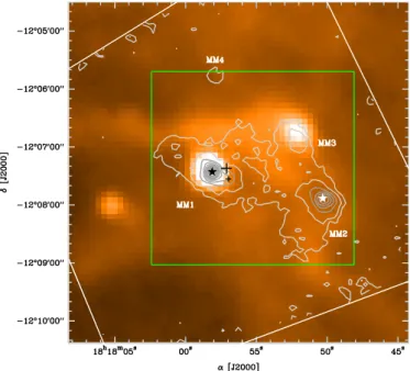
ob-Fig. 1. Image of the MSX 8µm emission toward IRAS 18151−1208 (color scale) overlaid with the 1.2 mm map (white polygon) by Beuther et al. (2002b) (white contours at 5 and 10 %, and grey con-tours from 20 % to 90 % of the maximum). The large and small crosses indicate the positions of the IRAS source and of MM1-SW (see text) respectively. The black and white star symbols show the positions of the methanol and water masers respectively. The green polygon dis-plays the region mapped in the present study (see Fig. 2).
Table 1. IRAS 18151−1208 sources characteristics. Offsets from IRAS position, J2000 coordinates and velocity in the local standard of rest (Beuther et al. 2002b) are reported.
source ∆α[&&] ∆δ[&&] α[J2000] δ[J2000] ![km/s] MM1 13.2 -4.9 18h17m58.0s -12◦07’27” 33.4 MM2 -98.9 -32.8 18h17m50.4s -12◦07’55” 29.7 MM3 -72.3 26.5 18h17m52.2s -12◦06’56” 30.7
served and can be modeled thanks to chemical network codes. It is even expected that chemistry could provide a reliable clock to date protostellar objects (e.g. van Dishoeck & Blake 1998; Doty et al. 2002; Wakelam et al. 2004).
After the description of the molecular observations and of the continuum data from the literature (Sect. 2), the results are presented in Sect. 3. Section 4 details the modeling proce-dure from the fits of the spectral energy distributions (hereafter SEDs) for MM1 and MM2 using MC3D1 code (Sect. 4.1.1
and 4.2.1) to the non-LTE calculations of the line profiles and intensities for all observed molecules using RATRAN2 code
(Sect. 4.1.2, 4.1.3, 4.2.2, and 4.2.3). In Section 5, we discuss the results of this detailed analysis in order to improve our ob-servational view of the evolution of high-mass cores from pre-stellar to high luminosity massive protostars.
1 See Wolf et al. (1999) for details.
Table 2. List of observational parameters for IRAM 30m and 22m Mopra telescopes. Here are indicated observed species, energy level transitions, line emission frequencies, half power beam width (HPBW), instrument (30m for IRAM-30m and Mo for Mopra telescope), main beam efficiency ηmb, receiver name, velocity resolution δ!, observation mode and system temperature Tsys.
Species Transition Frequency HPBW Instrumentd η
mb Receiver δ! Mode Tsys
[GHz] [&&] [m·s−1] [K] CS J = 2 − 1 97.9809 25 30m 0.78 A100 60 RaMa 260 J = 2 − 1 97.9809 32 Mo 0.49 3.5mm 191 OTFc 240 J = 3 − 2 146.9690 17 30m 0.69 D150 80 RaMa 420 J = 5 − 4 244.9356 10 30m 0.49 D270 96 RaMa 1150 C34S J = 2 − 1 96.4129 25 30m 0.78 A100 61 RaMa 190 J = 2 − 1 96.4129 32 Mo 0.49 3.5mm 194 OTFc ∼270 J = 3 − 2 144.6171 17 30m 0.69 D150 81 RaMa 390 CO J = 2 − 1 230.5380 11 30m 0.52 HERA 406 RaM2b ∼600 H2CO J = 303− 202 218.2222 11 30m 0.54 HERA 107 RaM2b 250 J = 322− 221 218.4756 11 30m 0.54 HERA 107 RaM2b 250 J = 312− 211 225.6978 11 30m 0.53 A230 104 RaMa 870 HCO+ J = 1 − 0 89.1885 36 Mo 0.49 3.5mm 210 OTFc ∼260 H13CO+ J = 1 − 0 86.7542 36 Mo 0.49 3.5mm 216 OTFc ∼175 N2H+ J = 1 − 0 93.1737 36 Mo 0.49 3.5mm 201 OTFc ∼180
aRaM – Raster Map mode set to create a 3 × 3 pixels mini-map with a ∆θ step of 10&&around source emission peak.
bRaM2 – Raster Map mode with HERA receiver, set to create a 190&&× 140&&map with a ∆θ step of 6&&towards MM1, MM2 and MM3.
cOTF – On-The-Fly observing mode carrying out on a 5&× 5&grid with an angle step ∆θ of 9&&and an OFF position at 30&from the center.
dConversional factor is S/T
mb=4.95 Jy/K for IRAM 30m telescope and S/Tmb=22 Jy/K for ATNF 22m telescope. 2. Observations.
Observations were performed during two sessions. The first one in June, 2005 at Mopra, the 22m dish of the Australia Telescope National Facility3 (ATNF). The second one in
August, 2005 at Pico Veleta, on the IRAM 30m antenna4.
2.1. Mopra observations
The IRAS 18151−1208 region was mapped in the On-The-Fly (OTF) mode in the rotational transition of CS (J=2−1) at 98.0 GHz, C34S (J=2−1) at 96.4 GHz , HCO+(J=1−0) at
89.2 GHz, H13CO+ (J=1−0) at 86.8 GHz and N
2H+(J=1−0)
at 93.2 GHz. Each run covered a field of 5&× 5&with a
half-power beam width (HPBW) of approximatively 36&& (ηmb =
0.49) and sampled with a ∆θ step of 9&&. We used the 3 mm
re-ceiver of the ATNF telescope with the digital auto-correlator set to the 64 MHz bandwidth with 1024 channels and both polarizations. It provides a velocity resolution of ∼0.2 km·s−1
over a 200 km·s−1range. Observations happened while weather
was clear, with a system temperature Tsys ∼ 175 – 260 K (see Table 2 for details). Pointing and focus adjustments have been set on Jupiter or known sources of calibration.
Raw data have been reduced with AIPS++ LIVEDATA and GRIDZILLA tasks (McMullin et al. 2004). LIVEDATA per-forms the subtraction between the SCAN spectra row and the OFF spectrum. Then it fits the baseline with a polynomial. We used the GRIDZILLA package to resample and build a data cube with regular pixel scale, weighted with the system tem-perature Tsys. We created a 39 × 39 grid of 9&& × 9&&pixel size
3 http://www.narrabri.atnf.csiro.au/mopra/ 4 http://iram.fr/IRAMES/index.htm
convolved by a Gaussian with a FWHM of 18&&, truncated at an
angular offset of 36&&. Finally, due to positional errors that we
found in maps, a shift in α of 14&&for N2H+, 10&&for CS and 5&&
for HCO+has been applied to fit millimeter-continuum peak
positions of the three sources given by Beuther et al. (2002b). 2.2. IRAM-30m observations
We observed the rotational transition of CO (J=2−1) molecule at 230.5 GHz and the two H2CO rotational para-transitions
(J=303−202) and (J=322−221) at respectively 218.2 GHz and
218.5 GHz simultaneously, using the HERA 3 × 3 pixel dual multi-beam receiver with VESPA backends at a resolution of 160 kHz for CO and 40 kHz for H2CO. Thus we built two
190&& × 140&& maps sampling every 6&& around MM1, MM2
and MM3. This observation was done while weather was good (τatm
0 =0.17), with Tsys∼ 600 K and 250 K for CO and H2CO
respectively. The maps are incomplete because raster mapping was not set to cover the entire ∆α and ∆δ, and the HERA ver-tical polarization (set for the CO) had a dead pixel (number 4). All pointings and focus have been set on suitable planets (i.e. Jupiter) or calibration sources.
The IRAS 18151−1208 region was also mapped in the rota-tional transitions of CS at 98.0, 147.0 and 244.9 GHz (J=2−1, J=3−2, J=5−4), in the isotopic C34S rotational transitions at
96.4 and 144.6 GHz (J=2−1, J=3−2) and in the H2CO
rota-tional ortho-transition (J=312 − 211) at 225.7 GHz, using
si-multaneously A100, A230, D150 and D270 receivers coupled to the high-resolution VESPA backend (resolution of 80 kHz). Central emission peaks of MM1, MM2 and MM3 were quickly mapped with a 3 × 3 raster position switching method with a
step of 10&&. Observations happened while sky conditions were
reasonable (τatm
0 ∼ 0.1–0.6 and Tsys∼ 260–1150 K).
Reduction for all IRAM 30m telescope data were per-formed with the CLASS software from the GILDAS suite (Guilloteau & Lucas 2000). We found and eliminated unusable data and treated platforming that appeared in CO and H2CO
baselines, then spectra at the same position were summed and finally antenna temperature T∗
a was converted into Tmb (see Table 2 for the values of ηmb).
3. Results
The modeling of the spectral energy distribution (SED) of a source is a common way to derive its density and temperature profiles (e.g. van der Tak et al. 1999). The obtained so-called physical model is then used as such to derive the abundances and to further investigate the physical properties (kinematics for instance) through the line emission modeling.
We thus observed CS, C34S, HCO+and H13CO+line
emis-sions which are bright and are tracing dense gas. We also ob-served H2CO line emission which traces dense gas and its
tem-perature. In additions we observed N2H+line emission which
is a cold gas indicator and finally CO that traces molecular gas flows.
3.1. Large scale maps: CO (2
−
1), H2CO (3
22−2
21),CS (2
−
1), HCO+(1−
0), H13CO+(1−
0) andN2H+(1
−
0)The velocity integrated maps in CO (2−1), H2CO (322−221),
CS (2−1), HCO+(1−0), H13CO+(1−0) and N
2H+(1−0) are
displayed in Fig. 2. Table 3 gives the derived emission exten-sions (at the 3σnoise level), the minor-to-major axis ratio b/a
and position angle (P.A.) of MM1, MM2 and MM3. Note that the C34S (2−1) MOPRA map was too noisy and was discarded.
The molecular emission always peaks at the positions of the three cores (millimeter-continuum peak positions by Beuther et al. 2002b). While MM1 and MM2 are always well detected, MM3 seems to be too weak in CS (2−1), H2CO (322−221) and
H13CO+(1−0) to be detected. The emission is extended even
between the cores for CS, HCO+ and CO lines but are more
peaked for N2H+, H13CO+ and H2CO lines. Some chemical
differences are already clear in CS, N2H+ and H2CO. While
MM1 is generally brighter than MM2, such as in the dust con-tinuum, MM2 has the same intensity in H2CO and is even
sig-nificantly brighter in N2H+than MM1.
CS (2−1) line emission is detected for MM1 and MM2 and weak emission could be present at 1σ for MM3. MM1 emis-sion is stronger than MM2, and covers a larger area, with exten-sions of 97&&× 81&&and 75&&× 62&&for MM1 and MM2
respec-tively. It indicates that a large scale envelope is surrounding MM1 and MM2. Axis ratios b/a are equal to 0.83 for MM1 and MM2, showing that the emission is almost spherical. The position angle of MM1 emission (+57◦) is similar to the
posi-tion angle of the large dust emission of +62◦given by Beuther
et al. (2002b). We note that emission is detected between MM1 and MM2. It suggests that they could be connected by a dense molecular filament.
The cold gas tracer N2H+(1−0) is detected toward the three
cores. Emission from MM2 is stronger and more concentrated than for MM1 (89&& × 62&& and 55&&× 54&& respectively),
sug-gesting that MM2 has a smaller and colder envelope. A simi-lar behaviour has been observed by Reid & Matthews (2007) for two similar cores in IRAS 23033+5951. The elongation of MM1 (b/a = 0.69) and position angle (+77◦) ressembles the
extension of the dust emission. MM3 line emission is stronger compared to other molecules and shows a connection with MM2. Together with a similar rest velocity for MM2 and MM3, it confirms that MM3 belongs to the IRAS 18151−1208 region. HCO+(1−0) and H13CO+(1−0) lines are detected for both
MM1 and MM2. MM3 has a weak emission in HCO+(1−0).
As for CS, MM1 emission is stronger and more extended than for MM2 (respective extensions are 104&& × 78&& and
57&&× 56&&). With b/a = 0.75 and a position angle of +75◦, we
note that MM1 emission may be extended along the outflow as expected since the HCO+ line emission is definitely showing
outflow wings such as in CO. The map shows an emission be-tween MM1 to MM2, and MM2 to MM3, confirming that the three sources are connected.
Dense gas traced by H2CO (322−221) line is detected for
MM1 and MM2 only. The emission from each source coin-cides perfectly with the dust continuum positions. MM1 and MM2 have similar intensities and have roughly the same small circular size (35&&× 30&&, b/a = 0.85 for the two sources) and
do not show any spatial suggestions of being contaminated by outflows.
The CO (2−1) line is detected in all sources and shows an extended emission from the whole region. MM1 emission is extended to the west (72&&× 51&&, b/a = 0.71 and P.A.= +85◦)
due to the red wing of the outflow (P.A.= +88◦). See the
fol-lowing section for more details on the CO outflows. 3.2. Molecular outflows in CO (2
−
1)The CO (2−1) line emission shows clear outflow wings. They are due to the already known CO outflow driven by MM1 (Beuther et al. 2002c) but seem also to be located in the re-gion of MM2. Figure 3 displays the average CO (2−1) spectra around MM1 and MM2, as well as the contour map of the in-tegrated emission in the wings. The displayed spectra clearly show emission wings up to high velocities. The observed maxi-mum velocities are -20.4 and +20.6 km·s−1for MM1 and -19.7
and +28.3 km·s−1 for MM2, with respect to !
LS R (see Fig. 3 and Table 4). It is clear from the map of this wing emission that there are actually two outflows driven by the two respec-tive cores. The MM2 outflow is actually newly discovered (see Sect. 5.1 for a discussion).
The MM1 outflow appears mostly east-west oriented. This is not quite the orientation observed for the main jet-outflow system recently discussed by Davis et al. (2004) with a NW-SE direction for the H2jet (see their Fig. 2). A second H2jet, west
of MM1 and probably driven by an embedded source in MM1-SW (see Fig. 1), is however also recognised in this work. The position of MM1-SW is marked in Fig. 3 with a small green tri-angle. Its location is close to a possible secondary center of
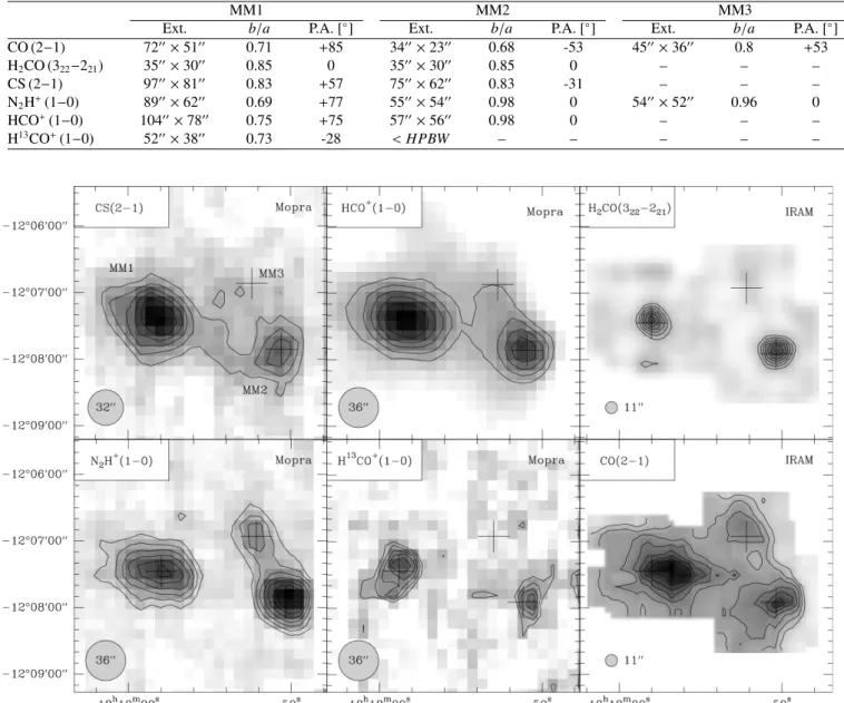
out-Table 3. Sources extension at 3σnoise, minor-to-major axis ratio b/a and position angle (P.A.; counterclockwise angle relative to the North) for each molecular transition observed. When the emission is almost spherical (b/a ≥ 0.85) P.A. is uncertain and set to 0◦.
MM1 MM2 MM3
Ext. b/a P.A. [◦] Ext. b/a P.A. [◦] Ext. b/a P.A. [◦] CO (2−1) 72&&× 51&& 0.71 +85 34&&× 23&& 0.68 -53 45&&× 36&& 0.8 +53 H2CO (322−221) 35&&× 30&& 0.85 0 35&&× 30&& 0.85 0 – – – CS (2−1) 97&&× 81&& 0.83 +57 75&&× 62&& 0.83 -31 – – – N2H+(1−0) 89&&× 62&& 0.69 +77 55&&× 54&& 0.98 0 54&&× 52&& 0.96 0 HCO+(1−0) 104&&× 78&& 0.75 +75 57&&× 56&& 0.98 0 – – – H13CO+(1−0) 52&&× 38&& 0.73 -28 <HPBW – – – – –
Fig. 2. Integrated velocity maps of CS (2−1), N2H+(1−0), HCO+(1−0), H13CO+(1−0) obtained with the Mopra 22m telescope (left and middle panels) and CO (2−1), H2CO (322−221) maps obtained with the IRAM 30m telescope (right panel). Level contours fit 90 % to 10 % of peak flux with a 10 % step. Only levels exceeding the threshold of 2σnoisein each map are plotted in order to identify detections. Peak fluxes are
16.9 K·km·s−1for CS, 16.9 K·km·s−1for N2H+, 32.9 K·km·s−1for HCO+, 2.31 K·km·s−1for H13CO+, 21.1 K·km·s−1for H2CO and 393 K·km·s−1 for CO. Crosses indicate the 1.2 mm continuum positions (Beuther et al. 2002b) for the three sources.
flow with a weak blue-shifted lobe in the south and the bright red-shifted western lobe being curved toward that location. The spatial resolution of our CO observation is not high enough to fully conclude about the association of CO outflowing gas with the different driving sources, but it seems that the western part of the MM1 outflow might actually be dominated by a second outflow from MM1-SW. The inclination of the MM1 flow on the sky is difficult to determine. From the significant extension of the flow and from the overlap of the lobes we can only say that the flow is neither face-on (in the plane of the sky) nor pole-on, and is therefore mostly intermediate.
The MM2 outflow is more compact than for MM1. Both lobes are confined in the core. The integrated emissions in the two lobes are similar in strength and are four times larger than the blue lobe of MM1. If the flow is dominated by a single ejection, the large overlap of the two lobes suggests that the flow is not face-on, but could be close to pole-on.
All the derived properties of the two outflows are summa-rized in Table 4. In addition, to quantify the energetics of the two detected outflows, we derive and give in this table the out-flow forces using the procedure described in Bontemps et al. (1996). The mechanical force (or momentum flux) seems to be the measurable quantity from observed CO outflows which can
approach in a not too uncertain way the corresponding quantity of the inner jet or wind(Cabrit & Bertout 1992; Chernin & Masson 1995). We estimate the outflow force FCOfor MM1
and MM2 by integrating the momentum flux inside vol-umes with radius 6&& and 18&& centered on the sources. In
addition, for the extended red lobe of MM1, a measurement is given between 18&&and 30&&to better cover the red lobe. Since
the inclination of the two outflows can not be reliably derived from such low resolution observations we adopt the average correction of a factor of 10 adopted by Bontemps et al. (1996). 3.3. Raster maps in CS, C34S, and H2CO (
3
12−2
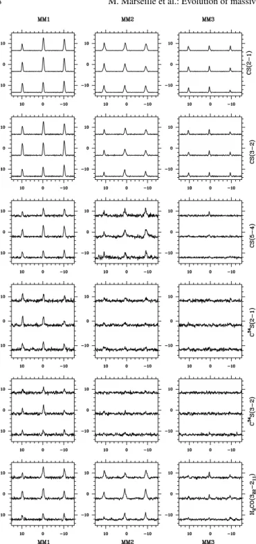
11)In addition to the large maps, a complementary investigation of the three millimeter sources is provided by the 3 × 3 raster maps of CS, C34S and H2CO (see Fig. 4).
All transitions are detected toward MM1 at !LS R =33.4 ± 0.1 km·s−1. The line profiles are similar with a typical line
width (FHWM) ∆! = 2.7 ± 0.2 km·s−1. CS (2−1), CS (3−2)
and CS (5−4) have roughly equal intensities. The optically thin C34S (2−1) line emission is detected all around the source at
an approximately constant intensity level of ∼ 1 K. In contrast C34S (3−2) seems to peak on the central position. The line
pro-files and the spatial patterns for H2CO (312−211) and CS (5−4)
are very similar, suggestive of common origin and excitation conditions for the two transitions (Eup/k are respectively equal to 33.40 and 35.27 K).
The intensities of most transitions toward MM2 are weaker than MM1. The line profiles at !LS R=29.8 ± 0.1 km·s−1have a triangular shape and a larger line width (∆! = 3.7 ± 0.1 km·s−1)
compared to MM1. This could be due to a gas motion contri-bution through its turbulence. The intensity of CS (5−4) is low compared to MM1, contrary to H2CO (312−211) line emission
which is as bright as in MM1.
All molecular line profiles are weaker in MM3, and seem to be less peaked than in MM1 and MM2 as seen in velocity integrated maps (cf. Fig. 2). They are detected at all positions in CS (2−1), (3−2), they have a weak emission in two positions in H2CO (312−211) and finally CS (5−4) and the C34S transitions
could not be detected. 3.4. Continuum fluxes
In order to derive the spectral energy distribution of the three millimeter peaks in IRAS 18151−1208, we retrieve continuum data from the literature. MM1 was imaged for the first time at 450, 800 and 1100 µm by McCutcheon et al. (1995) then at 450 and 850 µm by Williams et al. (2004), and the over-all region at 1.2 mm by Beuther et al. (2002b). Uncertainties are homogenized to account for typical calibration errors taken as 20 % in the millimeter range (1.1 and 1.2 mm) and 30 % in the submillimeter range (450 and 800 µm). In order to compare observations and model, we choose the deconvolved dust emis-sion size θr as a reference for the SED. We deconvolve using θr =
!
θ2s− θ2mbwhere θsis the observed mm-continuum half-peak size derived by Beuther et al. (2002b) and θmbthe HPBW
(11&&), using a two-dimensionnal Gaussian fit, assuming that
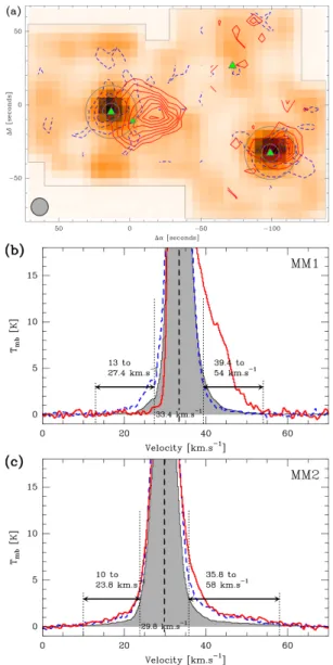
Fig. 3. (a) Contour maps of the CO (2−1) blue-shifted (dashed) and red-shifted (solid) integrated emission in the outflow wings for MM1, MM2, and MM3 (no detection). Positions of the MM cores are marked by filled (green) triangles. Blue- and red-shifted velocity intervals are +13.0 to +27.4 and +39.4 to +54.0 km·s−1for MM1, +10.0 to +23.8 and +35.8 to +58.0 km·s−1for MM2 and MM3. Lowest, highest con-tours and contour steps are (10, 70, 15) K·km·s−1(blue) and (60, 410, 50) K·km·s−1 (red) for MM1, and (10, 70, 15) K·km·s−1 (blue) and (20, 195, 25) K·km·s−1 (red) for MM2 and MM3. The background grey-scaled image is the integrated H2CO emission from Fig. 2. (b) CO (2−1) spectra for the MM1 outflow together with the velocity cuts used to integrate maps (dotted vertical lines) in (a) and to derive the mechanical forces. The solid line circles around MM1 and MM2 are 6&&and 12&&radius and indicate the area on which the FCO measure-ments are derived (see text for details). The filled grey spectrum is an average over the region of bright intensities in the wings as seen in the integrated map in (a). The dashed and blue (respectively solid and red) spectrum shows the line profile at the maximum of the blue (resp. red) lobe. (c) same as (b) for MM2.
the source is smaller than the beam and has a Gaussian shape. All millimeter (λ > 450 µm) peaks Sλpeakare then adapted to this reference size using
∆!b ∆!r FCOb FCOr FCOtotal Ext. blue Ext. red
[km·s−1] [km·s−1] [M
%·km·s−1·yr−1] [M%·km·s−1·yr−1] [M%·km·s−1·yr−1]
MM1 (13.0,27.4) (39.4,54.0) 0.44 ± 0.12 ×10⁻³ 1.86 ± 0.11 ×10⁻³ 2.30 ± 0.23 ×10⁻⁴ 17&&× 11&& 46&&× 45&& MM2 (10.0,23.8) (35.8,58.0) 0.48 ± 0.09 ×10⁻³ 1.86 ± 0.15 ×10⁻³ 2.34 ± 0.24 ×10⁻⁴ 40&&× 25&& 26&&× 22&& Table 4. Momentum flux of CO (2−1) calculated as in Bontemps et al. (1996). Blue and red integration intervals ∆!b,r(km·s−1), blue-shifted
momentum flux between 6&&and 12&& FCO
b(M%·km·s−1·yr−1), red-shifted momentum flux between 6&& and 12&& FCOr (M%·km·s−1·yr−1), total
momentum flux FCOtotal (M%·km·s−1·yr−1), maximal and outflows extensions are reported for MM1 and MM2.
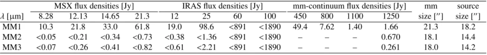
Table 5. Continuum flux densities of the three cores within IRAS 18151−1208 region. MSX flux densities are extracted from the catalog for MM1 and a 3σnoisecalculation over the beam is done to derive an upper limit for the undetected MM2 and MM3 sources. IRAS measurements
are derived from maps improved by HiRes method. Millimeter and sub-millimeter continuum flux densities are adapted to source reference size derived from continuum map by Beuther et al. (2002b).
MSX flux densities [Jy] IRAS flux densities [Jy] mm-continuum flux densities [Jy] mm source λ[µm] 8.28 12.13 14.65 21.3 12 25 60 100 450 800 1100 1250 size [&&] size [&&] MM1 10.3 21.8 33.0 61.8 19.0 98.6 <891 <1890 49.4 7.62 1.40 1.66 21.3 18.2 MM2 <0.05 <0.21 <0.34 <0.73 <0.38 <1.36 <891 <1890 – – – 0.670 18.1 14.4 MM3 <0.07 <0.26 <0.41 <0.82 <0.61 <2.21 <891 <1890 – – – 0.261 18.0 14.2 Sλ= " θr θmb #3+p Sλpeak (1)
where p is the density power-law index (derived by Beuther et al. 2002b) and Sλ the adapted flux density used to build
the SED. These flux densities are 49.4, 7.62, 1.40 and 1.66 Jy at respectively 450, 850, 1100, 1250 µm for MM1. The pro-cess is iterated on MM2 and MM3 and reference sizes with millimeter-continuum peak fluxes are reported in Table 5. Unfortunately the sub-millimeter continuum data for MM2 and MM3 are less abundant than for MM1 as these two sources were not observed by McCutcheon et al. (1995) and Williams et al. (2004).
Concerning mid- and far-infrared flux density measure-ments, MSX detected MM1 only. Thus we derive a 3σ noise level inside the beam size around the millimeter-continuum po-sition of MM2 and MM3, taken as an upper limit. We note that the IRAS emission of the region is dominated by MM1 which is confusing upper limits for MM2 and MM3. We therefore im-proved the IRAS map using the publicly available HiRes maxi-mum correlation method (Aumann et al. 1990), showing MM1 detection at 12 µm and 25 µm. At 60 µm and 100 µm, a sin-gle peak is detected slightly shifted to the west. We conclude that the huge beam width of IRAS sums the three flux densities from the three sources and the environmental filament contri-bution. Measured flux densities reported in the IRAS catalog at 60 µm and 100 µm are taken as upper limits for the three sources. All results are shown in Table 5.
4. Modeling the continuum and the molecular emission of MM1 and MM2
In this section we explain how we derive physical models for MM1 and MM2 and how we use them to investigate the
kinematics and the molecular abundances inside the cores. Following the method initiated and validated by van der Tak et al. (1999, 2000b) we use the dust continuum emission to derive the density and temperature profiles of the cores. Dust emission is sensitive to the total column density of dust (op-tically thin part of the SED in the millimeter wave range), and to the dust temperature and its distribution(mid to far-IR range). We try to build the simplest model in order to have the most general representation of the object. Then from the ob-tained physical model, we can run molecular line modeling to constrain kinematics (line profiles) and chemistry (abundances of observed species). Since MM3 is weak or not detected in a number of molecules and does not have a well constrained SED, we do not attempt to model it. We will restrict ourself to a simple discussion of its evolutionary stage.
4.1. IRAS 18151
−
1208 MM1 4.1.1. Spectral energy distributionThe MM1 core is massive (M ≈ 550 M% according to
Beuther et al. 2002b, and applying the correction of 1/2 from the associated 2005 erratum). It coincides with the bright IRAS 18151−1208 source (L ≈ 2.0 × 10⁴L
%). In first
approx-imation, assuming that the object has a spherical symmetry, we want to derive the best radial distribution of density and temperature that can fit the SED and that takes into account observational constrains.
(1) 1D modeling
We use the radiative transfer code MC3D in its 1D version (Wolf et al. 1999) to calculate the expected dust emission. This code is Monte-Carlo based, and is using the standard MRN (Mathis et al. 1977) dust grain distribution with the dust opaci-ties from Ossenkopf & Henning (1994). The model parameters are the central stellar luminosity L∗, its temperature T∗, the
in-Fig. 4. 3 × 3 maps in CS, C34S, and H2CO (312−211) for MM1, MM2 and MM3 sources. Velocity ranges from 15 to 50 km·s−1in all spectra, intensity ranges from −2 to 5 K for H2CO line emission, −1 to 2 K for C34S line emissions, −2 to 5 K for CS (5−4) line emission and −2 to 10 K for other CS line emission. Spectra have been smoothed to an identical velocity resolution of 0.2 km·s−1.
ternal and external radii r0and rextof the object, the molecular hydrogen density n0 at r0 and the power-law index p of the
density distribution of the form n(r) = n0(r/r0)p.
The bolometric luminosity is derived by integrating the SED, and we obtain Lbol = 1.4 × 10⁴ L%. The temperature
of the central star is taken as the corresponding main sequence star, i.e. T∗ =22 500 K (type B2V of 10 M%approximatively,
cf. Underhill et al. 1979). We adjust r0 to fit the dust
subli-mation radius where T + 1500 K. The external radius rextof the model is derived from the radius of the 1.2 mm contin-uum emission (here the deconvolved mean of major and minus axe given by Beuther et al. 2002b) assuming that the source has a Gaussian shape smaller than the beam size. The result-ing extension is 18.2&&, hence rext =27 300 AU or + 0.13 pc
at 3 kpc. The power-law index p is set to −1.2 according to the continuum profile fit by Beuther et al. (2002b). Finally the only free parameter left is n0and is derived by fitting optically
thin 1.2 mm continuum emission with a χ2 calculation. We
find n0 = 2.8 × 109 cm−3 at r0 = 21 AU with χ2 = 3.94,
hence ,n- = 8.0 × 105 cm−3 and a total mass of gas equal
to 660 M%. Outer and mean temperatures, formally Text and ,T-, are respectively 25.4 K and 27.3 K. The derived tem-perature profile can be fitted with a power-law of the form log10(T) = α. log r + β with α = −0.588 and β = 3.95.
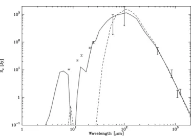
The resulting SED (see Fig. 5 in dashed line) shows that millimeter and sub-millimeter continuum parts are well modeled. On the contrary, the mid- and far-infrared emission is not reproduced, due to spherical symmetry that does not permit infrared photons, coming from inner parts, to leave the source without being reprocessed into photons at millimeter wavelengths. 2D modeling, where the polar regions contain less matter than in the mid-plane, should therefore reproduce better the observed mid-infrared emission.
(2) 2D modeling
We use the 2D version of the MC3D code which was de-veloped for disks. It is parametrized in radial and altitude di-rections (r,z) and it assumes the Keplerian disk equilibrium by Shakura & Syunyaev (1973):
n(r, z) = n0 (r r0 )p e−πc2z2·√2r ext·r−2.5 if r ∈ [r0; rext] 0 otherwise (2) We note that the model has three free parameters: n0
deter-mined as for the 1D modeling, the inverse height of scale c, and the source angle relative to the line of sight θlos. It is mostly θlos which controls the fraction of mid-infrared emission. Values close to 45◦ can roughly reproduce the SED, and we do not
further adjust the value to keep the model as general as pos-sible. The inverse height of scale c is controlling how thin the disk-like structure is. Since MM1 is young and is still mostly a spherical core, we try to keep c as small as possible while hav-ing always a significant mid-infrared emission for typical aver-age lines of sight. Thus c was gradually increased from 0.4 by 0.1 steps until an infrared emission greater than 0.1 Jy (limit of detection in the observations) could be obtained, finally leading to c = 0.7. Other parameters are kept identical as in 1D model (T∗, L∗, r0, rext and p). Calculations show that the best fit is obtained for n0 =2.7 × 109cm−3with χ2 =0.732 (total mass
M = 830 M%). The derived SED is plotted in Fig. 5 in
continu-ous line. It illustrates how a 2D modeling can reproduce better the observed infrared emission,although the silicate feature is not matched. We display the resulting density and temper-ature distributions in Fig. 6. One can see that the equatorial
Fig. 5. Spectral energy distributions obtained from 1D model (dashed line) and 2D model (continuous line) overlaid on observed fluxes of MM1 source. Dust continuum peak fluxes have been adjusted to fit radial extension of the model. Mid-infrared fluxes are obtained in 2D choosing a typical view angle θlos∼ 45◦(90◦=edge-on view).
Fig. 6. Density and temperature distributions for the 2D model pre-sented in a logarithmic grey scale, with 20 logarithmic levels from 102to 107 cm−3 for density and 10 logarithmic levels from 10 K to 263 K.
regions are denser and colder than around the polar axis. This is why mid-IR emission can escape and directly contribute to the SED.
4.1.2. CS and C34S line emissions
Since molecular line emission is usually dominated by the mostly spherical external layers of the protostellar cores, the 2D description might not be required to reproduce molecular lines.
We use the CS and C34S line emission to compare the
re-sults of modeling in 1D and 2D geometries. We directly use outputs of continuum models described above, assuming that dust and gas temperatures are equal, to which we add param-eters for molecular abundances and kinematics. The molecu-lar abundances relative to H2, X(CS) and X(C34S), mostly
de-termine the line intensities when the opacity is low (τ ! 1). Then we use a constant turbulent velocity !T. It is the main contributor to the line width compared to the thermal disper-sion. X(CS) and !T are therefore the free parameters to fit the intensities and widths of the line emission we observed. Finally we want to test if an infall motion in our model could
im-prove our results, giving at least an upper limit for it. The in-fall velocity is parameterized by the free-in-fall, power-law dis-tribution !in(r) = !in(r/r0)−0.5 (Shu 1977). We test its effect
on modeled line emission by switching between !in = 0 and !in =−0.4 km·s−1, the lowest value that modifies modeled line emission significantly for MM1.
The line profiles are computed with the RATRAN code (Hogerheijde & van der Tak 2000). This code allows 1D and 2D modeling using respectively multi-shell and grid descrip-tion of the object. The radiative transfer calculadescrip-tion uses the Monte-Carlo method to derive the populations of the energy levels and then builds data cubes that are convolved with corre-sponding beam sizes of the telescope to be directly compared with the observations.
In the 1D (spherical) geometry, a χ2 calculation is
per-formed for the optically thin C34S line (τ
2−1 =9.0 × 10⁻²and τ3−2 =2.2 × 10⁻¹) over a grid for fC34S=X(C34S)/X(C34S)typ (with X(C34S)typ=1.0 × 10⁻¹⁰) and !T. The best fit is obtained
for ( fC34S, !T) = (0.5, 1.0) with χ2 = 0.956. Then the grid is
refined for fC34Sonly, because model results are less dependent
of !T (kept equal to 1.0 km·s−1). The best result is obtained for fC34S = 0.51 with χ2 = 0.952, leading to the abundance
X(C34S) = 5.1 × 10⁻¹¹. Assuming a typical [S/34S] isotopic
ratio of 20 (Wilson & Rood 1994; Chin et al. 1996; Lucas & Liszt 1998) the CS emission is modeled with the abundance X(CS) = 1.0 × 10⁻⁹.
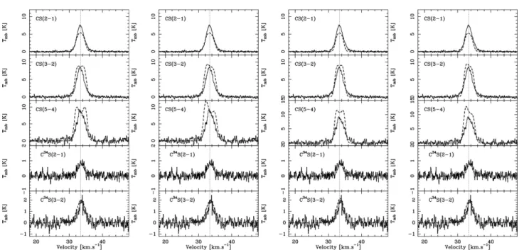
The final results of the line modeling are displayed in Fig. 7. Given the very small number (2) of free parameters, the result-ing fits are quite good. It reproduces well the line intensities. Only the profiles for the higher excitation lines indicate a sig-nificant difference between observations and this simple model. There are clear self-absorptions for the (3−2) and the (5−4) transitions (τ5−4=3.6) which indicate an overestimate of large
CS column densities for the highest excitation regions (central regions). This could well be due to a significant decrease of the CS abundance toward to the center of the core (see Sect. 5.5 for a discussion).
We find that a minimum infall velocity of −0.4 km·s−1 is
needed to start to see a clear asymmetric shape of the pro-file. Introducing infall improves only slightly the results for the (2−1) and (3−2) transitions and makes the fit of the (5−4) tran-sition worse (cf. Fig. 7, second plot from the left). We conclude that an infall velocity in the 1D model does not improve the fits, and we consider as an upper limit the value of −0.4 km·s−1.
For the 2D modeling, the same χ2adjustment is performed
for !Tand fC34S. Interestingly enough, the final best fit is exactly
the same than in the 1D geometry with X(CS) = 1.0 × 10⁻⁹
and X(C34S) = 5.1 × 10⁻¹¹. We note that line profiles and
relative intensities between the transitions are similar to the 1D case. Only a very slight improvement of the profile of CS (5−4) which is less self-absorbed can be noted. The result is shown on the third plot from the left in Fig 7.
Again the effect of an infall velocity on the line profiles is tested. With !in = −0.4 km·s−1 we note that the asymmetric profile of the line emission is less strong than in the 1D case (cf. Fig. 7, fourth plot from the left). We however conclude that infall in the 2D case does not improve critically the results.
Comparison between 1D and 2D modeling shows that us-ing a spherical description of the source is sufficient to re-produce CS and C34S molecular line emission, even if 2D is
slightly better with less self-absorption than in the 1D case. In addition we conclude that infall motion is not clearly detected and is not necessary to reproduce observations of MM1. We thus decide to use only 1D modeling without infall motion for the other observed lines.
The fact that 2D modeling is not needed for the CS line emission can be explained by the optical depth which is not so high at the corresponding frequencies compared with the mid-IR continuum, or by the asymmetry which is significant only on small scales where the temperature is high (between 300 and 1000 K). The observed molecular lines are not tracing these inner regions.
4.1.3. Other lines: N2H+, HCO+, H13CO+and H2CO
We adopt the 1D model derived in the previous section. For each molecule, the only free parameter left is therefore its relative abundance to H2.
(1) N2H+(J=1−0) modeling
The N2H+ (J=1−0) is split by hyperfine structure.
Theoretically there are 15 hyperfine components, which blend into seven for sources with low turbulence (Caselli et al. 1995) or into three if turbulence is strong, as in our case. In order to correctly fit observations from ATNF telescope at Mopra we created the molecular datafile for the RATRAN radiative transfer code. Energy levels, Einstein co-efficients Aul and collisional rates γul are derived from Daniel et al. (2004) through the BASECOL database maintained by the Observatoire de Paris5.
Energy levels included in the molecular datafile vary from J = 0 to J = 6. The hyperfine structure resulting from angular momentum and nuclear spin interaction (F1 and F quantum
numbers) leads to a total of 55 energy levels. The statistical weight of each level is determined by (see Daniel et al. 2005): nJ,F1,F =(2J + 1)(2F + 1)
[J, F1,F] (3)
where [J, F1,F] is the number of magnetic sub-levels for the
angular momentum J. The molecular data file takes into ac-count 119 radiative transitions where the first 15 of them fit to the (J=1−0) transition. The spectra obtained are then summed to finally reproduce the whole composite profile of the triplet (see Fig. 8).
Collision rates γulreported by Daniel et al. (2004) are given for helium as collision partner. As described by Sch¨oier et al. (2005) we take 1.4 × γulin order to correct for an H2collision
partner. Initially collision rates are given for temperatures from 5 K to 50 K which is the temperature range of the outer parts of our sources. To be able to model the entire sources, we have extrapolated the rates to high temperatures using a least-squares method that derives collisional rates from a
5 http://amdpo.obspm.fr/basecol/
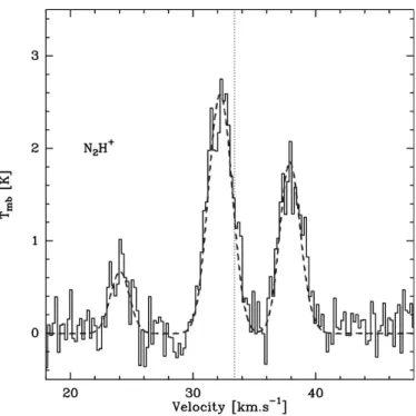
Fig. 8. Emission of N2H+from MM1 object overlaid by 1D model of the source (dashed line). The triplet shape is completely reproduced using our RATRAN molecular datafile. Spectra velocity resolutions are kept identical to observational resolutions reported in Table 2.
linear fit of the form:
log(γul) = a.log(T) + b (4)
This extrapolation has the advantage of fitting the global trend of the collisional rate without any exaggerated values for high temperatures.
Emission of N2H+is considered as optically thin (τ ∼ 10−2)
due to its typical low abundance. Thus we model it by com-paring the velocity integrated fluxes of observation and model starting from a typical abundance X(N2H+) = 1.0 × 10⁻¹¹.
The ratio of modeled to observed fluxes is then used to further correct the abundance while verifying that the line profile is always correctly reproduced. Iterating the process gives X(N2H+) = 3.5 × 10⁻¹⁰. An overlay of the model on the
observation is shown in Fig. 8.
(2) HCO+and H13CO+(J=1−0) modeling
The HCO+and H13CO+lines are good tracers of high density
gas and of its kinematics. H13CO+(J=1−0) is usually optically
thin (here we finally get τ = 3.4 × 10⁻²) so we adopt the
same routine to derive molecular abundances as for N2H+.
We then get an abundance of X(H13CO+) = 3.4 × 10⁻¹¹.
Applying a typical isotopic ratio [12C]/[13C] = 67 (Wilson &
Rood 1994; Lucas & Liszt 1998) we model the HCO+ line
with X(HCO+) = 2.3 × 10⁻⁹. Results are shown in Fig. 9.
The resulting modeled HCO+line is optically thick (τ = 1.7)
reaching a maximum intensity of ∼ 4 K. It suggests that the region of emission in the model is smaller than the telescope beam as expected for a high density tracer. On the other hand the observed intensity and profile are very different. It indicates that the bulk of the HCO+ rich gas does not follow
Fig. 7. Emission of CS and C34S from MM1 object (continuous line) overlaid by – from left to right – 1D static, 1D with infall (!
in =
−0.4 km·s−1), 2D static and 2D with infall (!
in =−0.4 km·s−1) model line emissions (dashed). Spectra velocity resolutions are kept
identi-cal to observational resolutions reported in Table 2.
(dust emission and optically thin lines). The HCO+(J=1−0)
line seems to have an excess on the blue side which could well be associated with the blue-shifted outflow wing which is mostly located inside the core in CO (see Fig. 3). Generally speaking, HCO+is a good outflow tracer and we speculate that
the HCO+line is actually dominated by some HCO+rich gas
associated with the outflow shocks inside the core (i.e. at high density as required to excite HCO+). This would mean that
the derived HCO+ abundance in the core envelope is only an
upper limit and could well be much smaller, except locally in outflow shocks.
(3) para- and ortho-H2CO modeling
The ratio between para and ortho populations of H2CO is an
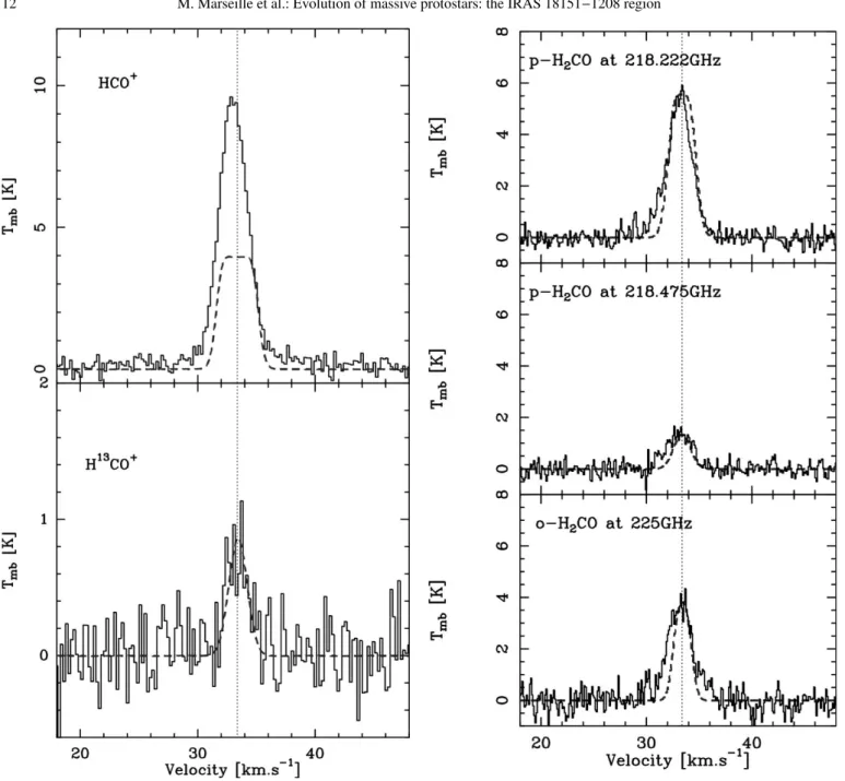
in-teresting parameter in the global context of gas temperature and chemical activity (Kahane et al. 1984) and can be a useful tool to follow chemical evolution of gas inside and between the ob-served sources. Our modeling indicates that the lines are mostly optically thin (τ218.2GHz=1.37, τ218.5GHz =0.09 and τ225GHz = 0.77) so we adopt the same routine as described for N2H+.
The abundances obtained are as follows X(para − H2CO) =
1.5 × 10⁻¹⁰and X(ortho − H2CO) = 1.3 × 10⁻¹⁰, leading to a
ratio para/ortho + 1.2. The agreement between the modeled and the observed lines is good. All the lines however tend to show some excess on the blue side, while the ortho line even shows excesses on both sides (see Fig. 10). In addition we want to emphasize that the two para-H2CO transitions which have two
significantly different Eup/k (respectively 21.0 K and 68.1 K) are well reproduced. This is an indication that the excitation temperature of the emitting gas is well reproduced by the phys-ical model.
4.2. IRAS 18151
−
1208 MM2 4.2.1. Spectral energy distributionSince MM2 is not detected in the mid-infrared, and taking into account our conclusions from the modeling of MM1, we de-cide to only model the source in a simple 1D, spherical geom-etry.We cannot derive the bolometric luminosity of MM2 by integrating its SED, due to the fact that all infrared fluxes are upper limits. Instead, we assume a luminosity of 2700 L%, which is uncertain by at least a factor of 2.
This luminosity corresponds to a B4V type star (approxi-matively 7 M%) with T∗=16 600K, that we use to describe
the heating source of our model. The 1.2 mm continuum de-convolved source extension from Beuther et al. (2002b) is equal to 14.4&& thus rext =21 600 A.U. or + 0.10 pc at 3 kpc and
we assume a power-law index p = −1.3 from the same paper. Because only one mm-wave peak flux density was measured for MM2 (see Table 5), we adapt n0to fit this unique
measure-ment. After two iterations we converge to n0=1.1 × 1010cm−3 at r0=12.4 A.U., hence ,n- = 1.1 × 106cm−3and a total mass gas of M = 460 M%. We derive Text =19.2 K, ,T- = 19.4 K and the temperature can be fitted by a power-law of the form log10(T) = α. log r + β with α = −0.614 and β = 3.85. The resulting SED does not show any emission in the mid- and far-infrared, in agreement with the observations (see Fig. 11) and as expected for a simple 1D description.
4.2.2. Molecular line emission modeling
We use the same procedure to model the molecular lines to-ward MM2 as for MM1. We therefore have derived the molec-ular abundance relative to H2, and the turbulent velocity !T. We have also tested a possible infall velocity field of the form !in(r) = !in(r/r0)−0.5.
Fig. 9. Emission of HCO+(top) and H13CO+(bottom) (J=1−0) from MM1 source overlaid by 1D model of the source (dashed line). Resulting abundances are X(HCO+) = 2.3 × 10⁻⁹and X(H13CO+) = 3.4 × 10⁻¹¹, according to the typical isotopic ratio [12C]/[13C] = 67. Spectra velocity resolutions are kept identical to observational resolu-tions reported in Table 2.
Emission of optically thin C34S lines (τ
2−1=4.4×10⁻²and
τ3−2=4.4×10⁻²) in MM2 object are treated by taking two dif-ferent grids for the χ2 calculation over its intensity and area.
The first grid is ( fC34S, !T) = ([0.1, 0.2...0.5], [1.5, 1.6...2.0])
and shows a best fit for ( f, !T) = (0.3, 1.7), the second one is finer with fC34S = [0.25, 0.26...0.35] and a fixed !T =
1.7 km·s−1because of the low dependence of the modeled line
on this parameter, compared to fC34S. It gives the best fit for
fC34S =0.27, hence an abundance X(C34S) = 2.7 × 10⁻¹¹. As
for MM1, the resulting modeled lines reproduce well all tran-sitions except the CS (5−4) line which is heavily overestimated
Fig. 10. para-H2CO (top and middle) and ortho-H2CO (bottom) emis-sions from MM1 source overlaid by 1D model of the source (dashed lines). Resulting abundances are X(para − H2CO) = 1.5 × 10⁻¹⁰and
X(ortho − H2CO) = 1.3 × 10⁻¹⁰, leading to a ratio para/ortho + 1.2. Spectra velocity resolutions are kept identical to observational resolu-tions reported in Table 2.
in intensity. Again it points to a lower abundance of CS in the inner regions compared to the outside.
Then, as above for MM1, we add an infall velocity profile following a typical r−0.5distribution. The asymmetric shape is
obtained for a minimum infall velocity !in=−1.0 km·s−1. The resulting profile is unchanged for (2−1) transition, is slightly improved for the (3−2) but shows an excess of blue emis-sion which is not observed for CS (5−4) (see Fig. 12, right). Therefore including infall velocity distribution does not im-prove our fit and hence does not seem to be necessary. It gives an upper limit for the infall velocity of !in=−1.0 km·s−1.
Fig. 11. Spectral energy distribution of MM2 overlaid with the 1D model result. Infrared emission has always an upper limit due to the non-detection of the source.
Fig. 12. Emission of CS from MM2 object overlaid by 1D static (left) and 1D with infall (!in =−1.0 km·s−1) model of the source (dashed
lines). Spectra velocity resolutions are kept identical to observational resolutions reported in Table 2.
The optically thin emission of N2H+ (τ ∼ 10−2) in MM2
is treated by comparing the observed and modeled velocity in-tegrated area and using it to adapt an initial typical abundance (1.0 × 10⁻¹⁰). The resulting fit for N2H+ is shown in Fig. 13
and corresponds to X(N2H+) = 6.3 × 10⁻¹⁰. As for MM1, the
quality of the fit is high.
For HCO+ and H13CO+ we obtain the following
abun-dances: X(HCO+) = 5.1 × 10⁻⁹and X(H13CO+) = 7.6 × 10⁻¹¹.
The best fit result is shown in Fig. 14. As for MM1, the mod-eled HCO+ line emission does not reproduce well the
obser-vations. The HCO+column density derived from the H13CO+
line implies an heavily saturated (τ = 19) HCO+line which is
not observed. Obviously in contrast to all the other molecules, the distribution of HCO+does not follow the simple spherical
geometry of the model.
Fig. 13. Line emission of N2H+from MM2 object overlaid by the 1D model of the source (dashed line). Spectra velocity resolutions are kept identical to the observational resolutions reported in Table 2.
We then derive the best abundances for the para and ortho-H2CO to reproduce the three observed transitions (see Fig. 15).
The abundance obtained for the ortho transition at 225 GHz is X(ortho − H2CO) = 2.0 × 10⁻¹⁰. For the two para
tran-sitions, no unique abundance can be derived. For the best fit of the 218.222 GHz line emission, the abundance obtained is X(para − H2CO) = 2.6 × 10⁻¹⁰ but the 218.475 GHz line is
then too weak by a factor of almost 2; see Fig. 15. At the other extreme, if the 218.475 GHz line is fitted, the abundance ob-tained is X(para − H2CO) = 4.8 × 10⁻¹⁰. In contrast to MM1
for which a correct ratio of the two para lines was obtained, the modeled ratio (218.222 over 218.475) for MM2 appears to be too large. Since the weaker 218.475 GHz line emission has a higher upper energy level (Eup/k = 68.1 K) it suggests that the emitting gas is actually warmer in MM2 than what is rep-resented by the simple 1D model. The resulting para to ortho ratio is therefore in the range + 1.3– 2.4.
5. Discussion
5.1. MM2: a new massive protostar driving a powerful outflow.
MM2 is a millimeter source without infrared counterpart (MSX or IRAS). It is even seen in absorption over the local back-ground in the MSX 8µm image (see Fig. 1). A water maser has been detected toward the core by Beuther et al. (2002a). With the addition of our newly discovered CO outflow driven by MM2, it all clearly points to a protostellar nature of MM2. Inside the core size of 0.22 pc (14.4&&, see Table 3.4) a total
mass of 460 M%is obtained with MC3D (dust emissivity for
the MRN grain distribution; see Table 6). MM2 is therefore a newly discovered massive protostellar core which is not de-tected in the mid- or far-IR: an IR-quiet massive protostellar object. A more complete comparison with the detailed analysis
Fig. 14. Emissions of HCO+(top) and H13CO+(bottom) (J=1–0) from MM2 source overlaid by 1D model of the source (dashed line). Spectra velocity resolutions are kept identical to observational resolutions re-ported in Table 2.
obtained for low-mass protostars and in Cygnus X by Motte et al. (2007) is given in the following section.
5.2. Evolutionary stages of MM1, MM2 and MM3. In contrast to low-mass star formation (e.g. Andr´e et al. 2000), the evolutionary sequence for high-mass stars is not well con-strained and understood. The general lack of spatial resolution leads to discussions of evolutionary sequences mostly applied to massive clumps (such as HMPOs, typical size of 0.5 pc) or to high-mass dense cores (typical size of 0.1 pc) which cannot usually be directly compared to protostars which have physical sizes more of the order of 0.01−0.05 pc (e.g. Motte et al. 1998; Motte & Andr´e 2001). A recent attempt to clarify these differ-ent scales and associated evolutionary sequences is compiled in Motte et al. (2007); see their Table 4. From the complete sur-vey of the relatively nearby Cygnus X complex, a total of 40
Fig. 15. para-H2CO (top and center) and ortho-H2CO (bottom) emis-sions from MM2 source overlaid by 1D model of the source (dashed lines). Spectra velocity resolutions are kept identical to observational resolutions reported in Table 2.
high-mass dense cores were recognized with an average size of 0.13 pc, similar to sizes of nearby, low-mass dense cores but 20 times more massive and 5 times denser. These high-density cores were all found to be already protostellar in nature and were proposed to well represent the earliest phases of high-mass star formation. Among the 40 cores, 15 were already as-sociated with an UC-H region and bright in the infrared, 8 were only bright in the infrared, and 17 were IR-quiet proto-stellar cores. This sequence is proposed to be mostly an evo-lutionary sequence, the IR-quiet cores being the precursors of the IR-bright cores, and then of UC-H regions. We will dis-cuss the cores in IRAS 18151−1208 in the framework of these recent Cygnus X results.
MM1 MM2
L 14 000 L% 2 700 L%
T∗ 22 500 K 16 600 K
Mgas 660 ± 130 M% 460 ± 100 M%
rext 27 300 A.U. 21 600 A.U.
n0 2.8 (0.6) × 109cm−3 1.1 (0.2) × 1010cm−3 ,n- 8.0 (2.0) × 105cm−3 1.1 (0.2) × 106cm−3 p -1.2a -1.3a Text 25.4 (0.5) K 19.2 (0.4) K ,T- 27.3 (0.2) K 19.4 (0.2) K α −0.588 (0.011) -0.614 (0.012) β 3.95 (0.03) 3.85 (0.04) rin 21 (2) A.U. 12 (1) A.U. !T 1.0 (0.1) km·s−1 1.7 (0.1) km·s−1 X(CS) 1.0 (0.3) × 10−9 5.4 (1.5) × 10−10 X(C34S) 5.1 (1.4) × 10−11 2.7 (0.8) × 10−11 X(N2H+) 3.5 (0.8) × 10−10 6.3 (1.4) × 10−10 X(HCO+) 2.3 (0.7) × 10−9 5.1 (1.6) × 10−9 X(H13CO+) 3.4 (1.1) × 10−11 7.6 (2.4) × 10−11 X(p-H2CO) 1.5 (0.4) × 10−10 2.6 (0.7)–4.8(1.3) × 10−10 X(o-H2CO) 1.3 (0.4) × 10−10 2.0 (0.6) × 10−10 [para/ortho] + 1.2 + 1.3–2.4
aValues from continuum map analysis by Beuther et al. (2002b).
Table 6. Summary of results from dust continuum emission model-ing (above mid-line) and from molecular line emission modelmodel-ing (be-low mid-line). The relative uncertainties on the derived parameters are given inside the parentheses and are at the 3 σ level. They correspond to the rms noise propagated through the modeling process. The addi-tional absolute uncertainty on masses and abundances, mostly due to the uncertain emissivity of dust, is given in Sect. 5.3.
First of all no bright radio source is detected in the whole IRAS 18151−1208 clump. All the massive protostellar objects detected in the clump are necessarily objects in an evolutionary stage prior to the formation of an UC-H region. In Fig. 1, the distribution of mid-infrared emission from MSX is displayed. It is clear that the main bright infrared source is associated with MM1 while the MM2 area is devoid of mid-infrared emission. The core is actually even seen in absorption over the local back-ground. MM3 is more complicated since a moderately bright MSX source is situated close to the center of the core.
MM1 has a mass of 660 M%in a radius of 27 300 A.U. (core
size of 0.27 pc) obtained from the fit of the SED with MC3D (Table 6). It has a bolometric luminosity higher than 104 L
%,
and is bright in the mid-IR (S20 µm=61 Jy). It drives a powerful
bipolar outflow and therefore hosts at least one mid-IR bright massive protostar. Using the same dust properties (millime-ter dust emissivity and average temperature) as in Motte et al. (2007), and inside a 0.13 pc size, the MM1 core would have a mass as high as 74 M%, and would therefore be among the most
massive cores of Cygnus X. With an equivalent S20 µm=190 Jy
at 1.7 kpc (distance of Cygnus X), it would be the brightest core which is not associated with an UC-H region (see Fig. 7 in Motte et al. 2007). It is however not as bright in the mid-IR as the well-known AFGL 2591 source described by van der Tak
et al. (1999). In the Motte et al. (2007) classification, MM1 is therefore a high-luminosity IR (or IR bright) protostar.
Except its non detection in the mid- and far-IR (S20 µm !
2 Jy), the properties of MM2 ressemble those of MM1. It has a mass of 460 M%in a radius of 21 600 A.U. (core size of 0.22 pc)
obtained with MC3D (Table 6), a still high bolometric luminos-ity of 2700 L%, and it drives a powerful bipolar outflow. Using
the same dust properties as in Motte et al. (2007), and inside a 0.13 pc, the MM2 core would have a mass of 45 M%, and would
therefore be among the 40 high-density cores of Cygnus X. In the Motte et al. (2007) classification, MM2 is a mid-IR-quiet massive protostar.
Observations of MM3 does not permit to conclude defini-tively on its nature. Although it is massive with a flatter density profile (about 200 M%and p = 0.8, (Beuther et al. 2002b) and
no outflow detected, any mid-IR emission is confused due to the nearing confusing source detected by MSX and the pres-ence of a bright IR filament in the background. At best one can only propose that MM3 is a probable prestellar core.
One can also use the CO outflow energetics to further dis-cuss the evolutionary stages of MM1 and MM2. Outflows are believed to be the best indirect tracers of protostellar accre-tion. Interestingly enough, while MM2 is not a bright IR source and is less luminous than MM1, its CO outflow is as power-ful as the one of MM1. This is like Class 0 low-mass proto-stars which have on average more powerful outflows than more evolved, and IR bright Class I objects. It has been interpreted by Bontemps et al. (1996) as due to a decrease of the accretion rate with time. Extrapolating these results to higher masses, we investigate in Fig. 16 how MM1 and MM2 place in the evolu-tionary diagram based on the energetics of CO outflows. The location of the low-mass protostars (Class 0 and Class I) is dis-played with stars and is well reproduced by a toy model (dot-ted tracks) based on an exponential decrease of the accretion rate with time (see details in Bontemps et al. 1996) for stars between 0.2 and 2 M%. Three additional tracks are given for
M = 8, 20, 50 M%. One can note, for instance, that while
the low-mass protostars reach a maximum luminosity which is higher than their final ZAMS luminosity (by a factor of 5 for 0.2 M%stars) the luminosities of massive protostars are
al-ways increasing. In this scenario, the dashed line would repre-sent the location of the transition between Class 0 and Class I protostars, i.e. the location where half of the final mass is ac-creted (first black arrow symbols, second arrow symbols are for 90 % of the mass accreted). If this can be extrapolated to high-mass protostars it indicates that MM2 is younger than MM1 and could host a high-mass Class 0 like protostar. Note that the HMPO (star symbols) including MM1 and MM2 are not well resolved as individual collapsing objects. This is partic-ularly important for MM2 for which the measured luminosity depends on its continuum fluxes in the millimeter range and therefore directly scales with the size of the region. The lumi-nosity of MM2 should therefore be seen as an upper limit of the actual luminosity of the protostar. In this diagram, MM2 and MM1 are located in the area of the M = 20 M%track with
MM2 having less than 50 % of its final mass, and MM1 hav-ing of the order of 50 % of its final mass accreted. While the stellar embryo of MM2 is therefore certainly not yet a ionising