Air leakage of Insulated Concrete Form houses

(1)

Air Leakage of Insulated Concrete Form Houses

by

Hannah Durschlag

Bachelor of Science in Civil Engineering, 2010 Northwestern University

Evanston, IL

Submitted to the Department of Architecture in partial fulfillment of the requirements for the degree of

Master of Science in Building Technology

at the

Massachusetts Institute of Technology

June 2012

Signature of Author……….. Department of Architecture May 11, 2012

Certified by……… John Ochsendorf Associate Professor of Architecture and Civil and Environmental Engineering Thesis Co-‐Supervisor

Certified by……… Leslie Keith Norford Professor of Building Technology Thesis Co-‐Supervisor

Accepted by………... Takehiko Nagakura Chair of the Department Committee on Graduate Students

(2)

Thesis Co-‐Advisor: John Ochsendorf, PhD

Associate Professor of Architecture and Civil and Environmental Engineering

Thesis Co-‐Advisor: Leslie Keith Norford, PhD Professor of Building Technology

(3)

Air Leakage of Insulated Concrete Form Houses by

Hannah Durschlag

Submitted to the Department of Architecture

On May 11, 2012 in partial fulfillment of the requirements for the degree of Master of Science in Building Technology

Abstract

Air leakage has been shown to increase building energy use due to additional heating and cooling loads. Although many construction types have been examined for leakage, an exploration of a large number of Insulated Concrete Form (ICF) houses has not yet been completed. This thesis first collects 43 blower door tests of recently built ICF houses in North America. These are then examined and compared with a large collection of blower door tests of wood-‐stud construction. There is a 1.2% difference between ICF and wood-‐stud air leakage, with a very similar range. This range is mainly attributed to leakage from the attic space and cracks around windows based on a thorough investigation of two specific ICF houses in Nashville, TN. Using an EnergyPlus building model, the difference in air leakage between a typical ICF and wood-‐stud house in Chicago and Phoenix is not found to cause a significant gap in energy use. However, the range in air leakage does affect the amount of energy a single-‐family house consumes.

Thesis supervisor: John Ochsendorf

Title: Associate Professor of Architecture and Civil and Environmental Engineering

(4)

Acknowledgements

First, I would like to acknowledge Professors Ochsendorf and Norford. Thank you for the support and advice. You made it possible for me to come to MIT as a civil engineer and leave as a building scientist.

I would also like to recognize the Building Technology Lab. The people I have met here are both colleagues and friends. I greatly admire all the work that you do. In particular, thank you to Amanda Webb for contributing her expertise for Chapter 5 of this thesis.

This thesis would not have been possible without funding. Thank you to the Concrete Sustainability Hub and the Building Technology Department for supporting this work.

I would like to thank my friends, particularly the Northwestern Eight, for being there for me and always being able to make me laugh. I am so glad you are in my life.

Finally, a big thank you to my parents. I appreciate your constant love and support more than I can say.

(5)

1. Introduction

1.1 Understanding building energy use

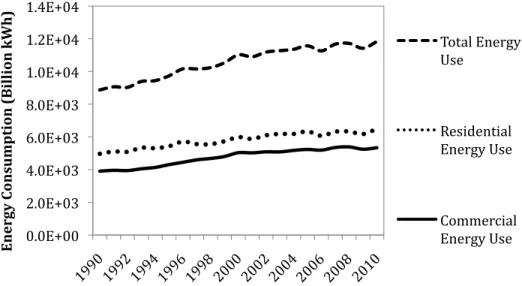
According to the Environmental Protection Agency, buildings consumed 39% of the total energy used in the United States in 2003 (EPA, 2009). The chart in Figure 1.1 displays the residential, commercial, and total energy use since 1990. A large portion of total energy use in the US is due to buildings. Energy use is increasing with time, but the percentage of building usage remains fairly consistent.

Figure 1.1 Total and building energy consumption in the United States illustrates the increase in energy use over time for all sectors (EPA, 2009).

In addition, approximately 44% of building energy in 2003 was used for heating and cooling (EPA, 2003). According to Balaras et al. (1999), the structure of a building and its corresponding design affect energy loss and consumption. Therefore, by understanding how design decisions influence heating and cooling loads, buildings can be modified to reduce energy consumption.

1.2 Air leakage

There are many aspects of building structure that can affect energy use. This thesis will focus on air leakage. A typical definition of air leakage is the movement of air into and out of unplanned openings in a building enclosure or envelope (Sherman and Chan, 2004). Examples of unplanned openings include cracks around windows or joints between the wall and the roof. A test used to measure the size of these holes is called a blower door test. This test determines the volume flow rate through cracks, the infiltration, and their total area, the leakage area. The blower door test will be explained in detail in Chapter 2.

Air leakage is the focus of this thesis due to its importance in energy loss and consumption. As will be examined in much more detail in the literature review in Chapter 2, between 16 and 33% of building energy consumption has been attributed to infiltration (Shaw and Jones, 1979) (Emmerich and Persily, 1998) (Sherman,

0.0E+00 2.0E+03 4.0E+03 6.0E+03 8.0E+03 1.0E+04 1.2E+04 1.4E+04 En er gy C on su m p ti on ( B il li on k W h ) Total Energy Use Residential Energy Use Commercial Energy Use

(7)

1985). In other studies, infiltration is responsible for between 7 and 46% of energy loss (Tamura and Shaw, 1977) (Balaras et al., 1999). These ranges are large and are associated with different types of structures and climates. Therefore, more precise numbers for specific building envelopes would be useful for making design decisions.

1.3 Insulated Concrete Form (ICF)

Due to the large percentage of building energy used by the residential sector, this thesis will focus on single-‐family housing. There are many different construction methods for single-‐family housing. Wood-‐stud construction is the most typical. Houses can also be built from cast-‐in-‐place concrete, pre-‐cast concrete, structural insulated panels, Insulated Concrete Form (ICF), and other options. This thesis will examine ICF single-‐family construction. The basic structure of ICF is two layers of two and one half inches polystyrene insulation, which are held together with metal or plastic ties. Concrete, generally six inches thick, is then poured between these two layers. The insulation acts as permanent formwork for the concrete and is not removed (Insulated Concrete Form Association, 1995). A representation of this geometry can be seen in Figure 1.2.

Figure 1.2. A schematic (left) and picture (right) of the Insulated Concrete Form which displays two layers of insulation, tied together. These act as permanent formwork for a layer of concrete (Rajagopalan et al., 2009) (http://www.concrete-‐home.com, 2006).

This thesis investigates ICF construction for several reasons. First, as will be shown in the literature review in Chapter 2, the air leakage of insulated concrete form houses has not yet been examined in detail. Next, because of the inherent continuity of the walls in ICF construction, there have been numerous claims of its potential for energy savings due to lower air leakage (ICF Facts, 2012) (ARXX ICF, 2012). There is clearly a hole in our knowledge of this building type that is necessary to address.

1.4 Structure of thesis

As described above, neither the air leakage of ICF houses nor their energy use has been examined in detail. This thesis examines three key questions:

(8)

1. What are the trends in air leakage of ICF single-‐family houses and how do they compare to the air leakage of wood-‐stud construction?

2. What characteristics of the houses explain the variability in air leakage within ICF construction?

3. How does this variability affect the energy use of ICF houses when compared to wood-‐stud construction?

Chapter 2 of this thesis examines previous work done on air leakage of different construction types and their effect on energy use. It presents studies most relevant to the questions above and reveals topics that have not yet been explored.

The goal of Chapter 3 is to investigate the first question, above. First, blower door tests of 43 ICF houses in seven states are conducted. This is larger than any other collection of ICF air leakage data. The resulting set of information consists of infiltration and leakage area data, along with characteristics about each house. Chapter 3 provides an analysis of the trends in this data and the characteristics of the houses that best predict air leakage. This chapter also includes a comparison of the air leakage of ICF houses with an existing data set of conventionally built homes. These are generally assumed to be wood-‐stud construction.

Chapter 4 more fully explores the variability of the air leakage data introduced in Chapter 3. This process involves examining the leakage sites of two houses from the data set, one that is unusually leaky and the other unusually tight. By understanding where these houses leak and the relative sizes of the holes, the differences between them can be identified. Not only will this explain why there is a range in leakage area of ICF houses, it will establish the important leakage sites as well.

Finally, Chapter 5 will develop an energy simulation of a typical US house. Using the comparison of ICF and wood-‐stud construction air leakage completed in Chapter 3, reasonable values of air leakage will be input. The results will display how infiltration affects energy use in two different climates, Chicago and Phoenix.

Chapter 6 will identify the primary conclusions of this thesis and their importance.

1.5 Summary

This introduction identifies the importance of energy use in single-‐family residential houses. It also motivates the roles air leakage and insulated concrete form have in the discussion. Finally, the three main questions of this thesis and how they will be answered are presented.

(9)

2. Literature Review

2.1 Introduction

This chapter reviews previous work done on air leakage and insulated concrete form houses. It begins with a review of the definitions, physics and quantification of air leakage. Then, literature on concrete structures, leakage sites and how infiltration affects energy use will be summarized. This will guide the work towards the final goal of understanding the air leakage of insulated concrete form houses, its uncertainty, and its effect on energy use.

2.2 Basics of air leakage

Air leakage, or infiltration, is the movement of air in and out of a house through unplanned openings (Sherman and Chan, 2004). Because this air must be heated or cooled, this phenomenon can cause a large amount of unnecessary energy use. According to Shaw et al. (1973), air leakage depends on wall design, materials used, workmanship, and the condition of joints.

Pressure differences between the indoors and outdoors induce infiltration. The most common method of estimating the volumetric airflow rate through a building is seen in Equation 2-‐1, which is a generalized form of the orifice equation.

€

Q = cΔP

n where

Q = the volume flow rate, m3_/s c = the flow coefficient, m3_/s/Pa

∆P = the indoor/outdoor pressure difference, Pascals n = the pressure exponent, dimensionless

There are two weather phenomena that can create this pressure difference: temperature and wind. Air temperature determines changes in air pressure with height, so a temperature difference between indoor and outdoor air can create a pressure differential, which drives infiltration. In addition, the wind can change the pressure on the outside of a building positively or negatively, depending on building and wind characteristics (ASHRAE Fundamentals, 2009).

The value of n is based on the type and properties of the opening. If the Bernoulli equation is used, which assumes the leak has a short path and frictional forces can be ignored, n = 0.5. This value is used if there is a high Reynolds number because inertial forces are much greater than viscous forces. If the flow rate is low, there will be losses due to friction. This causes the flow rate to be linearly proportional to the pressure and therefore n = 1.0. Generally, n is found to be at a value in between 0.5 and 1.0 (Sherman and Chan, 2004).

The most common method of air leakage measurement is fan pressurization, when a fan installed in a doorway creates a uniform pressure across a building envelope. There are three different methods of fan pressurization: create several different pressures and measure the flow of air through the fan at each; create a volume (2-‐1)

(10)

change on the inside of a building and measure the pressure response (AC pressurization); provide one pressure pulse to the building and view the decay (pulse pressurization) (Sherman and Chan, 2004).

The first method is the most common, and will be the only one addressed and used in this research. ASTM E779 describes how to determine air leakage from these measurements (ASTM, 2003). This procedure, summarized below, quantifies infiltration in two ways: flow and leakage area. Flow is the volume of air flowing through the holes in the outer envelope when the home is at a specified pressure difference. Generally, the infiltration is reported at a pressure difference of either 50 Pascals, where an accurate reading can be made, or extrapolated to 4 Pa, which is a typical condition. It is generally reported in m3_{/s.
Leakage
area
is
the
size
of
the} holes in the outer envelope of a building, typically in units of cm2_{.
The
procedure
to} determine the volume flow rate and the leakage area is:

1. Install a fan in the doorway and increase the pressure in a house from 10 to 60 Pascals in steps of 5 or 10 Pa. Measure the flow through the fan at each pressure.

2. Correct the airflow for the difference in outside and inside density.

a. Inside and outside temperature and elevation are necessary for this calculation.

3. Take the natural log of both the pressure and the corrected airflow.

4. Calculate the variance in these two sets of data and the covariance of both sets.

5. The exponent in the orifice equation described above, n, is the covariance divided by the variance of the natural log of pressure.

6. Calculate c, according to Equation 2-‐2:

€

c = e

ln( flow)−n*ln( pressure )

7. Correct c for the difference in indoor and a reference viscosity. 8. Calculate leakage area using Equation 2-‐3:

€ AL = C0* P₀ 2 * 4 n −.5

Every house has a different value of volume flow rate and leakage area. Because these houses have some differing attributes that may contribute to the difference in air leakage, it is typical to normalize by these characteristics. For example, the most common way to normalize volume flow rate is to divide it by house volume. This eliminates the effect the difference in house volume has on leakage area – a larger house would intuitively have a larger envelope and therefore more leakage sites – and the resulting numbers can be compared without considering this difference.

When flow rate is divided by house volume, a metric known as air changes per hour is found, as seen in Equation 2-‐4. Essentially, the number of air changes per hour is (2-‐2)

(11)

how many times, in one hour, all of the air in a house is turned over and replaced by outside air. € ACH = Q Volume* 3600s hour where

ACH = air changes per hour, h-‐1 Q = flow, m3_/s

Floor area and surface area can both be used to normalize leakage area. The most common method is seen in Equation 2-‐5, where both attributes are used.

€

NL = 1000 *

A

L

A

f

H

2.5m

⎛

⎝

⎜

⎞

⎠

⎟

0.3 where

NL = Normalized Leakage, dimensionless AL = Leakage area, cm2

Af = Floor Area, m2 H = Height, m

Although the leakage area is a property of a building, the flow rate varies with temperature and wind speed. In order to calculate flow from leakage area without experimental results, Sherman and Grimsrud developed an equation in 1980, separating temperature from wind effects. This can be seen in Equation 2-‐6 (Sherman and Grimsrud, 1980).

€

Q = AL

1000 * CSΔt + CWU

2

This equation uses the leakage area, AL, the temperature difference, and the wind speed to calculate flow rate. In addition, the stack coefficient, CS, is based on the height of the house and the wind coefficient, CW, is derived from height and shelter class. This equation is commonly used in energy modeling, when temperature and wind speed are input every hour in order to achieve more accurate results. A similar, although slightly more complex, version is used in this thesis and will be introduced in Section 5.3. According to Al-‐Homoud (2004), in addition to temperature differentials and wind velocity, infiltration depends on tightness of construction, exterior shielding, and building height. Therefore, Equation 2-‐6 captures all of the elements that lead to airflow.

2.3 Infiltration of concrete structures

Persily et al. (2006) completed the most recent analysis of the largest set of air infiltration data in the United States: the Lawrence Berkeley National Laboratory database. They then calculated representative values of normalized leakage, which can be seen in Table 2-‐1. These values are for houses across the US, and therefore are generally wood-‐stud construction (Persily, 2006). This is a very complete (2-‐4)

(2-‐5)

(12)

analysis and should represent typical houses. However, they did not consider how different types of envelopes may affect the air leakage of a house.

Table 2-‐1. Representative values of normalized leakage based on the LBNL database (from Persily (2006) Table 5)

Becker (2010) compares different types of concrete walls for their air tightness. He finds that autoclaved aerated concrete block walls are tight when compared to regular and lightweight aggregate concrete block walls. However, a layer of lime-‐ cement coating can reduce the air changes per hour significantly. Although this is a reasonable conclusion, it does not deal with insulated concrete form, the envelope this thesis examines, nor does it examine non-‐cementitious options.

Several studies compare concrete buildings with other building types. This thesis will primarily focus on studies in the United States. Shaw et al. (1973) find that tile and plaster walls are generally more leaky than concrete and steel, but that concrete and steel do not seem to differ greatly. Persily (1999) concludes that frame and masonry buildings may be slightly leakier than concrete, panel, manufactured, metal and curtain wall envelopes. Although these conclusions are valid, these studies do not examine insulated concrete form envelopes.

Kosny et al. (1998) references a study by Southwest Infrared Inc., which states that blower door tests of 7 ICF houses show that ICF houses are inherently tighter. This study was not available online, through the MIT libraries, or from the author. However, a dataset consisting of seven points seems quite small to make any conclusion about tightness. It is not clear if these houses are similar in design, in the same climate zone, or the same age. However, Kosny et al. use the air tightness found for the ICF houses and then a 20% larger value for wood homes. This is a large assumption given the small size of the data set.

On a more specific level, Petrie et al. (2002) observe two side-‐by-‐side homes, one made from ICF and one built from a wood frame. They compare them using flow rates from blower door testing. On average, the ICF house leaks 0.345 m3_{/s
and
the} conventional house leaks 0.390 m3_{/s.
Therefore,
there
is
typically
a
difference
of} 0.045 m3_{/s
at
50
Pa.
To
put
this
in
perspective,
using
a
standard
house
floor
area
of} 222 m2_{times
3
m
in
height,
the
passivhaus
standard
of
.6
ACH
at
50
Pa,
which
is}

!"#$%&'()*+,)%-%.)+/#)%+0*'$)12'"1&)223+ 4)%#+56'&7+ 8&""#+%#)%+&)22+79%1+

:;<=>+$?_+0:>@@+A7?₃₊ 8&""#+%#)%+$"#)+79%1+_:;<=>+$?_+0:>@@+A7?₃₊

5)A"#)+:B;@+ :=?B+ @=C<+

:B;@D:B>B+ :=@E+ @=;B+

:BFBD:B<B+ @=>C+ @=E>+

(13)

considered very low, allows 0.111 m3_{/s.
The
difference
between
ICF
and
wood} found by Petrie can now be considered quite small, which is a legitimate result. The authors attempt to account for variation in the data by redoing the blower door tests in reverse order. There is no process of understanding how ICF houses can vary by construction crew, climates, or age, for example.

Several studies have also found that infiltration does not vary based on wall construction. Shaw and Jones (1979) concludes that wall constructions do not correlate with differences in air leakage. In addition, in his master’s thesis, Doebber (2004) describes the large amount of controversy related to this topic. Although he does assume that the standard normalized leakage value for wood-‐framed houses is lower than the one for concrete homes, 1.21 versus 0.76, he is unsure if this assumption is legitimate. There does not seem to be any study that examines a large data set, understands its variability, and reaches a strong conclusion on the air leakage of ICF compared to wood frame houses.

2.4 Air leakage variability

In this thesis, the study of variability is generally connected to the study of leakage sites. Differences in air leakage are typically attributed to differences in location or size of leakage sites.

There is a body of literature on where leaks occur and their size. One study by Kalamees et al. (2008) does a blower door test and then uses infrared imaging to see where the air is leaking on several different buildings (2008). However, they only use the results to identify typical locations, as opposed to comparing the variability among the buildings.

Nagda et al. (1986) constructs two identically leaky homes and retrofits one of them. However, he does this by purposely omitting 11 different typical methods of tight construction. This is not realistic and only captures the tightening of purposely-‐ leaky sites as opposed to typically leaky sites. He is able to reduce the air leakage by approximately 35% through retrofitting. Although this shows that retrofitting can be useful, it does not teach the audience about unknown leakage sites.

Another idea used in several studies is sequential blower door testing. Nabinger and Persily (2011), Gammage et al. (1986), and Gettings (1988) all perform blower door testing, retrofit the building and then blower door test again to determine the contribution of the leakage sites to air infiltration. Nabinger and Persily (2011) install house wrap and fix leaks in the floor, Gammage et al. (1986) investigate the ductwork, and Gettings (1988) caulks, adds weatherstripping, installs door jambs/sweeps and seals other locations with foam and tape. Although the results exhibit the contribution of these locations, the studies either do not distinguish among the different types of retrofits -‐ they perform them at the same time and do a blower door test after they have all been completed -‐ or only examine one component such as ductwork.

(14)

Dickerhoff et al. (1982), Bassett (1986) and Armstrong et al. (1996) use a similar method and separate the different possible leakage sites to understand how much each contributes to the total leakage. For example, Dickerhoff et al. (1982) measures 34 houses in Atlanta, Georgia, Reno, Nevada and San Francisco, California. Based on these homes, they find that ductwork, electric gaskets, the fireplace, the kitchen exhaust vents and the bathroom exhaust vents contribute 13%, 1%, 24%, 6% and 3%, respectively, to the air leakage. In addition, there is a collection of study results in ASHRAE (The American Society of Heating, Refrigerating and Air-‐Conditioning Engineers) Fundamentals (2009). A summary of leakage contributions, which will be further discussed in Chapter 4, is:

• Walls: 35%

 This includes cracks between components such as top plates, outlets, and plumbing penetrations

• Ceiling details: 18%

 Including recessed lighting • HVAC systems: 18%

• Fireplaces: 12% • Vents: 5%

• Diffusion through walls: <1%

Again, although interesting, these results do not compare different types of buildings. There is a lot more that can be learned from the data collected for this summary.

Finally, there is a large collection of air leakage contributions of individual components. Each part of a building has a leakage associated with it. A comprehensive list can be found in the master’s thesis by Frye (2011). Reinhold and Sonderegger (1983) uses this type of data and shows very good agreement between leakage area determined by summing components and the whole house blower door test results.

The idea that the number of leakage sites can account for differences in total leakage is similar to the approach taken in this thesis. In Chapter 4, differences in the type and number of leakage sites are compared to explain uncertainty in air leakage.

2.5 How infiltration affects energy use

2.5.1. Percent of energy consumption due to infiltration

Shaw and Jones (1979) finds that 29% of heating loads are due to air infiltration based on a survey of 11 schools. Sherman (1985) states that approximately one third of energy use is due to infiltration. VanBronkhorst (1995) reports based on a study of 25 office buildings that 15% of heating load consumption is due to infiltration, while cooling requirements do not depend on air leakage. Finally, Emmerich and Persily (1998) find that between 16 and 29% of heating and cooling loads are due to infiltration. This paper also investigated 25 office buildings. Unfortunately, the wide breath of types and quantities of buildings studied makes it

(15)

difficult to come to a unique number. In addition, these results are all from data. It would be interesting to understand how much influence infiltration has when using energy modeling for a typical building. This is discussed further in Section 2.5.3, where there is a review of studies on changes in energy use due to air leakage, some of which use energy models.

2.5.2. Percent of energy loss due to infiltration

Another way studies report their findings is the percent of energy lost due to infiltration. This may be the same statistic as discussed above, if it is assumed that the occupants make up for the energy lost by consuming more. However, if their home is simply colder or warmer, this may not be the case. Tamura and Shaw (1977) find that infiltration causes between 22 and 46% of heat loss (1977). Balaras et al. (1999) find that between 7 and 25% of heat loss is due to infiltration (1999). Overall, these statistics are somewhat similar to the energy consumption numbers above and do not include energy models.

2.5.3. Changes in energy use due to infiltration

There are several studies that report the change in energy use due to changes in infiltration. First, Emmerich et al. (2005) reduce infiltration from 0.17 -‐ 0.26 to 0.02 -‐ .05 air changes per hour on a two-‐story office building, a one-‐story retail building and a four-‐story apartment building in an energy simulation. This is an 83% reduction, on average. They find a 40% energy savings for gas use and a 25% energy savings for electricity use. Although these results are reasonable, this study does not examine single-‐family houses, which are the topic of this thesis.

Purdy et al. (2001) increase the infiltration from 1.5 to 3 air changes per hour in a simulation of a specific house, and observe a 27% increase in the heating load. However, the house modeled represents a typical energy efficient house in Canada. This does not further our understanding of conventional US homes.

In a study mentioned above, Kosny et al. (1998) use a smaller infiltration rate when simulating typical ICF and stud houses. They find that a reduction of infiltration by 20% in an ICF home causes a heating and cooling energy reduction of 4% in Miami and 6.5% in Washington D.C. As discussed above, this assumption is based on a dataset of 7 houses, which is small for any substantial conclusions.

Petrie (2002), also discussed above, finds that ICF construction is less leaky than wood-‐stud by comparing two in-‐situ houses using blower door testing. The only other difference between these homes is the thermal resistance, because ICF construction has a slightly greater R-‐value. By monitoring them for 11 months without occupation but on a simple operating schedule, it is found that the ICF house uses 5.5% -‐ 8.5% less energy. However, because the houses differed in both leakiness and conductivity, the difference in energy use cannot be solely attributed to air infiltration differences.

(16)

Finally, Nabinger and Persily (2011) reduce the air leakage by 18% in a single, unoccupied manufactured house through retrofits. They note an energy consumption drop for heating and cooling of 10%. However, this is not a typical US house.

As seen in all of the above examples, whether based on simulation or monitoring, reduction in infiltration can cause a significant drop in energy consumption. However, none of the studies use the simulation of a typical US house with values of air leakage that are based on substantial evidence.

2.6 Conclusions

This chapter finds that:

1. There is currently no study that compares the air leakage of a large collection of ICF and wood-‐stud construction single-‐family houses.

2. Although there has been research done on leakage sites, no study uses this information to understand variability among houses with different types of envelopes.

3. Many papers examine the energy associated with infiltration, but none use the simulation of a typical US house with justifiable values of air leakage.

These findings directly relate to the questions introduced in Chapter 1. This thesis will add to our understanding of each of these aspects of air leakage and energy in Chapters 3, 4 and 5, respectively.

(17)

3. The Air Leakage of Insulated Concrete Form Houses

3.1 Introduction

As seen in the literature review, extensive research has been done on the air leakage of houses. The leakage of different construction materials has also been compared. However, there does not appear to be any previous examination of a large collection of insulated concrete form houses. Comparing two houses can be useful, but this lacks consideration towards variability. This chapter presents new results on:

1. A collection of blower door tests and characteristics of ICF houses

2. An examination of the trends in this data including its distribution, variability, and characteristics which best predict air leakage

3. A comparison of the ICF air leakage data to the air leakage of conventional US houses, which are generally considered to be wood-‐stud construction

3.2 Experimental results from blower door testing

To address the lack of information on the air leakage of ICF houses, blower door tests were conducted on 43 ICF houses. Data was also collected on characteristics of the houses. The purpose of this section is to understand what data is collected, and then organize, categorize and visualize it. The code written for this analysis can be found in Appendix A.

3.2.1 Methodology

The blower door tests include information on the following items. These are based on the survey form found in Appendix B.

• Flows and pressures, with the ducts both opened and closed

• The temperature, before and after the test, both indoors and outdoors • House geometry

 Volume  Floor area  Height

 Perimeter measurements • Window and door size and number • The HVAC system

 Type

 Supplies and exhausts • Location and year built

• The consultant who performed the test

• The leakage area, CFM at 50 Pascals, and ACH reported by the consultant

The locations and distributions of the collected dataset can be seen in Figure 3.1. Although the set does not have a large geographic range, the number of data points is considered satisfactory for analysis.

(18)

Figure 3.1 The location and distribution of the data collected on insulated concrete form houses is large enough for analysis.

In total, there were 43 tests conducted in seven states. However, three of these are removed because they do not include the original flow and pressure measurements, including one from Arizona, New Hampshire and Ontario. In addition, ten tests in Mississippi measure a set of attached row houses. These homes are very similar in results, as though one house was sampled many times. Because there are only 30 other points, the dataset appears to favor this specific leakage area. This is considered unsatisfactory, and only one of these ten points is left in the data set; the median is selected. These ten points will be explored later in this chapter to understand the variation due to quality control of the builder and random variation. The final number of data points is 31.

Using the flows and pressures, ASTM E779 Standard is used for each house to calculate a leakage area. Appendix C contains the results, as well as the height and floor area of each house.

3.2.2 Results

The histogram in Figure 3.2 on the left includes the leakage area data for all 43 houses, in centimeters squared. The histogram on the right in Figure 3.2 is the air leakage data with 12 tests removed, as described above. The x-‐axis displays the center values of the bins and the values above the bars are the number of data points in that bin.

5" 10" 2" 12" 8" Ontario:"4" 1" 1"

(19)

Figure 3.2. The histogram of air leakage of all the houses (left) and the histogram of the final 31 houses (right) display that air leakage of ICF houses favors the lower end of the range.

3.2.3 Discussion

For both charts in Figure 3.2, the numbers favor the lower end of the range. The average value of the 31 points in Figure 3.2 (right) is 793 cm2_{.
There
are
few
houses} at the upper end of the air leakage spectrum.

The house with the very large air leakage does not seem to have any unusual attributes. There may have been some problem in conducting the test. For example, if a window is open, the amount of air leakage during the test might be very large.

3.3 Leakage distribution

It is considered important to explore the distribution of the data for several reasons. First, a large aspect of this thesis is comparing ICF leakage to the US housing stock. In order to understand their relationship, it is necessary to compare their distributions. In addition, by examining the distribution, the variability of the ICF air leakage is scrutinized. Because the ultimate goal of understanding the air leakage is controlling it, the variability is important. Another aspect of this work that adds to the understanding of variability is the analysis of the duct air leakage. It will be shown that the overall variability of the data is demonstrated in this analysis. Finally, in Chapter 5 of this thesis, the energy use of ICF houses is quantified for different leakage areas. In order to use representative values of leakage area, the distribution of the data must be understood.

3.3.1 Methodology

The first task is to determine the distribution of the data. The method of maximum likelihood is employed to calculate the parameters of the most fitting distribution, which is hypothesized based on a visual inspection (Rice, 2007) (Matlab, 2011). These results are compared with the original values using the Kolmogorov-‐Smirnov test, which determines, non-‐parametrically, if two datasets are statistically different (Stephens, 1974) (Matlab, 2011). Using a non-‐parameteric test is important because a t-‐test, for example, assumes a normal distribution. Then, the parameters found are used to randomly generate a PDF, which can be visually compared to the data itself.

243 492 741 990 1239 1488 1737 1986 2235 2484 0 2 4 6 8 10 12 14 16 18 Air Leakage, cm2 Number of Houses 243 492 741 990 1239 1488 1737 1986 2235 2484 0 1 2 3 4 5 6 7 Air Leakage, cm2 Number of Houses 17 7 6 4 5 1 1 0 0 1 7 6 6 4 5 1 1 0 0 1

(20)

There are three methods for understanding the variability of the data. First, the data is bootstrapped – random samples are taken – and the mean is taken of each sample. The spread of these means indicates how variable the data is and how affected it is by outliers (Rice, 2007). Second, as part of the ASTM standard to calculate air leakage, the method of determining uncertainty is reported. For example, each air leakage is a number plus or minus its uncertainty. A summary of this method can be found in Appendix D (ASTM E779).

Finally, using the series of row houses removed from the data set, the range in air leakage of houses with all of the same measured characteristics can be calculated. This range is due to a combination of the quality control of the builder and random variation of quantities that are not measured in this dataset.

The code written for this analysis can be found in Appendix E.

3.3.2 Results: The distribution and variability

Based on a visual inspection of the histogram in Figure 3.2, the parameters of a gamma distribution are calculated using the method of maximum likelihood to describe the data. For the gamma distribution, Matlab uses the PDF found in Equation 3-‐1. € y = f (x | a,b) = 1 baΓ(a)x a −1_e −x b

The parameters a and b for the data in this study are 2.38 and 333.79, respectively. At the 5% significance level, this gamma distribution describes the experimental data well. Figure 3.3 displays an overlay of the gamma distribution, created using the parameters found above, on the data.

Figure 3.3. A histogram of the air leakage with a gamma distribution overlaid. The gamma distribution has parameters a = 2.38 and b = 333.8 and is a good fit for the ICF air leakage data.

243 492 741 990 1239 1488 1737 1986 2235 2484 0 1 2 3 4 5 6 7 8 Air Leakage, cm2 Number of Houses data gamma (3-‐1)

(21)

The next step is to understand the variability of the data. Using the 31 data points being analyzed, the range in leakage area is 2500 cm2_{.
However,
there
is
one
leaky} outlier in the leakage area data, based on Matlab’s default definition of an outlier. This definition uses the quartile range and a constant multiplier. The multiplier is based loosely on a normal distribution. However, Walpole et al. (2007) state that the constant used by Matlab is typically applied to any box and whisker plot. Therefore this outlier can be removed to achieve a range in leakage area of 1514 cm2_{,
with
a} mean of 732 cm2_.

However, this does not explore all the methods of examining variability at our disposal nor does this indicate any of the causes of variability. The following discussion describes the results of three methods of understanding the variability in the air leakage data.

First, the data itself is bootstrapped, and the mean is calculated of each sample. The histogram can be seen in Figure 3.4 and displays a range of 800 cm2_.

Figure 3.4 The means of samples from the dataset are in groups of ten, taken 1000 times. The mean of all the data, 793, is in the middle of the distribution with variability of approximately 400 cm2_.

The second method is through the ASTM E779 standard, which describes a process for calculating the uncertainty of air leakage, as discussed in Appendix D. The chart in Figure 3.5 displays a histogram of all of the uncertainties. In general, these values are smaller than 300 cm2_.

467 548 628 709 789 870 950 1031 1111 1192 0 50 100 150 200 250 Number of Houses Leakage area, cm2 Mean%=%793%cm2%