An Aging society : opportunity of challenge

Digitized

by

the

Internet

Archive

in

2011

with

funding

from

Boston

Library

Consortium

Member

Libraries

working paper

department

of

economics

AN AGING SOCIETY: OPPORTUNITY OR CHALLENGE David M. Cutler James M. Poterba Louise M. Sheiner Lawrence H. Summers No. 553 _{May 1990}

massachusetts

institute

_of

technology

50

memorial

drive

Cambridge, mass.

02139

AN AGING SOCIETY: OPPORTUNITY OR CHALLENGE David M. Cutler James M. Poterba Louise M. Sheiner Lawrence H. Summers No. 553 May 1990

.s\

AN AGING SOCIETY: OPPORTUNITY OR CHALLENGE

David M. Cutler and James M. Poterba

Massachusetts Institute of Technology

Louise M. Sheiner and Lawrence H. Summers

Harvard University

April 1990

We are grateful to George Akerlof, Robert Barro, Bill Brainard, Greg Duffee,

Rachel Friedberg, Ken Judd, Larry Katz , Laurence Kotlikoff, George Perry,

Julio Rotemberg and Robert Solow for helpful comments and to the National

Science Foundation and Alfred P. Sloan Foundation for research support. A

An Aging Society: Opportunity or Challenge?

David M. Cutler, James M. Poterba, Louise M. Shelner, and Lawrence H. SumiDers

SuiiuTiarv

The American population and that of the industrialized world is aging

rapidly. The suggestion is commonly made that increases in saving are

necessary to prepare for increases in future dependency. This paper argues to

the contrary that demograhic change represents as much of a macroeconomic

opportunity as a challenge, and that ceteris paribus, the appropriate policy

response to recent and projected demographic change is a reduction in national

saving. However, demographic changes are not nearly large enough to justify

the sharp decline in U.S. national saving during the 1980s.

Our analysis proceeds in five steps. First, we note that estimates

of the coming dependency burden need to recognize that the share of dependent

children in the population will fall, that the labor force will grow more

productivity as it matures, and that a more slowly growing labor force will

require less investment to maintain a given degree of capital intensity.

Taking account of these factors, it appears that the consumption cost of

demographic change over the next 60 years will be less than 10 percent. This

is equivalent to a .1-.2 percent per year slowdowTi in productivity growth, or

about three times as large as the "peace dividend" the economy will enjoy over

the next decade.

Second, we obser\'e ' that the good news

—

reduced labor force growth and

fewer dependent children

—

comes before the bad news of increased dependency.

Furthermore, saving for increases in the dependent population encounters

diminishing returns as labor force growth slows. Using a stylized Ramsey-tj-pe

optimal growth model, we find that the appropriate policy response to future

demographic changes is a reduction in national saving. This conclusion is

robust with respect to a variety of assumptions about preferences, technology,

and the demographic future.

Third, allowing for international capital mobility reinforces our

conclusions. Because labor growth decelerates faster and dependency increases

come more quickly abroad, demographic factors push toward making the U.S. a

cpaital importer over the next decade. This drives down rates of return,

making increased saving less attractive.

Fourth, in a more speculative vein we consider the response of technical

change to changes in labor force growth rates. Contrary to the often-asserted

d^Tiamism hj'pothesis that young populations are better able to innovate and

thus grow more quickly, we find using international comparisons that a

reduction in labor force growth is likely to be associated with an increase in

the rate of productivity growth.

Fifth, we assess the implications of our results for fiscal policy.

Demographic change appears likely to raise private saving in the near term,

weakening the case for higher governEent saving. Arguments that efficiency

considerations related to "tax smoothing" require accumulation of a Social

Security trust fund are shown to be quantitatively unimportant.

Ve conclude by arguing that while a Social Security trust fund may be

justified as a politically convenient way -to raise the American national

An American woman reaching childbearing age in 1960 would expect 3.5

children; an identical woman in 1990 would expect only 1.9 children. This

dramatic demographic change makes it almost inevitable that the American

population will age rapidly over the next 50 years. By 2025, the share of the

American population over 65 will exceed the share of Florida's population that

is aged today. The ratio of the number of retirees to the number of workers

will have risen by nearly two-thirds. Even more dramatic demographic changes

are occuring abroad. The share of the Japanese population that is over 65

will rise from 11% to 19% over the next two decades. If current fertility

levels are maintained until 2050, the population of Vest Germany will not only

age but will shrink by more than one-third.

These demographic changes have aroused considerable anxiety. Economic

concerns have focused on the burden that increased dependency will place on

the economy in general and the Federal treasury in particular, as well as on

the possible loss of dynamism that will occur as population growth slows.

Concern about increased dependency has led to a potentially radical change in

American fiscal policy. To insure that Social Security taxes will be

sufficient to fund benefits over the next 75 years, and to help the nation

save in anticipation of increased demographic burdens, the Social Security

legislation enacted in 1983 calls for Social Security taxes to exceed benefits

over the next 30 years. This surplus will be accumulated in a trust fund,

which will peak at 29% of GNP in 2020 and then be drawn down as the population

ages .

This paper steps back from the current political debate over the Social

Security trust fund and examines the more general question of how serious a

macroeconomic problem aging represents and how policy should respond to it.

2

do not consider the broader question of whether the current U.S. national

saving rate is too high or too low, but focus on the partial effect of

demographic changes on the optimal level of national saving. In addition, we

consider the effects of demographic change on productivity growth and the

optimal timing of tax collections.

Our general conclusion is that demographic changes will improve American

standards of living in the near future, but lead to modest reductions over the

very long term. Ceteris paribus. the optimal policy response to recent and

anticipated demographic changes is almost certainly a reduction rather than an

increase in the national saving rate. Slowing population growth will reduce

the investment that must be devoted to equipping new workers and housing new

families, while making it easier for the United States to attract foreign

capital. While there are many reasons for arguing that the United States

currently saves too little, anticipated demographic change is not one of them.

Our analysis proceeds in five steps. First, we assess the magnitude of

the coming dependency burden. While it is true that the share of the

population that is over 65 will increase sharply, it is also true that the

share of children in the population will decline over time, and that the

fraction of the labor force that is near peak productivity will increase.

Using information on projected fertility, mortality and labor force

participa-tion rates as well as data on health care costs and the spending of different

age groups, we assess past and future dependency trends. We find that

demographic changes unaccompanied by changes in capital intensity would reduce

per— capita incomes by between seven and twelve percent over the next sixty

years, but would actually increase incomes over the next twenty years. In

only one of the next six decades will demographic changes have as large an

3

decade. The decline in living standards caused by the increased dependence

would be fully reversed by a .15% per year increase in productivity growth.

Second, we consider the consequences of the slower labor force growth

that presages the increase in the retired share of the population. Between

2010 and 2060, the labor force is expected to decline slightly, compared with

an average increase of 1.6% annually between 1950 and 1990. The projected

decline in the labor force growth rate will permit a three to four percent

reduction in the share of net investment in total income without reducing

capital intensity. Since reduced labor force growth will occur before

dependency burdens increase, projected demographic changes raise the

short-term consumption path even if the steady— state consumption level declines. We

show that in a standard growth model with plausible parameter values, optimal

consumption typically rises in response to a demographic shock like that

experienced in the United States over the last three decades.

Third, we consider the implications of integrated world capital markets

for our analysis. The degree and speed of population aging in the other major

OECD countries, particularly West Germany and Japan, is more dramatic than

that in the United States. This increase in dependency in the rest of the

OECD will coincide with a deceleration in labor force growth rates. This

means that along an optimal path, the rest of the world will export capital to

the United States. This tends to increase U.S. consumption and reduce saving

in the short run relative to the path that would obtain if capital were

internationally immobile.

Fourth, we go beyond the standard growth theoretic approach and ask

whether demographic changes are likely to affect the rate of technical change.

4

technical change. Such effects would sharpen our conclusion that diminished

fertility represents an opportunity rather than a problem. Using

inter-national cross-section time series data for the 1960-1985 period, we find some

evidence that countries with slower labor force growth experience more rapid

productivity growth. The estimates suggest that the reduction in labor force

growth projected for the next forty years may raise productivity growth enough

to fully offset the consequences of increased dependence. These results are

uncertain. A more definitive finding is the absence of any support for the

pessimistic view that aging societies suffer reduced productivity growth.

Fifth, we consider the implications of our results for fiscal policy.

Since demographic changes over the next decades are not likely to be

associated with reduced private saving, our analysis suggests that they do not

present a reason for reducing the budget deficit. There remains the question

of efficiency in tax collection. Maintaining current service levels for the

elderly will require an increase in government spending from about 32 to 37%

of GNP. Since the deadweight loss from taxation rises with the square of the

tax rate, financing these expenditures on a pay as you go basis will involve

higher deadweight losses than maintaining a constant tax rate. We find

however that these effects are likely to be small, amounting to at most

several tenths of a percent of annual GNP.

We conclude by discussing the implications of our results for Social

Security, intergenerational redistribution more generally, and for population

and immigration policy. Our findings suggest that population aging does not

constitute a strong argument for the accumulation of a large Social Security

trust fund, although if national saving is deemed to be inadequate for other

5

1. The Burden of Increased Dependency

The economic consequences of population aging depend on the nature of the

underlying demographic change as well as the relationship between the resource

needs of individuals at different ages and their capacity for self-support.

This section presents our estimates of the economic burden of increased

dependency, noting the uncertainties associated with each step in the

calculation.

1.1 Changing Demographic Structure

Figure 1.1 plots the Social Security Administration's projections of the

number of persons aged 65+ as a fraction of the population aged 20-64 between

1950 and 2050. Figure 1.2 plots the total dependency ratio, the number of

children plus elderly as a fraction of the working age population. The

figures show the Social Security Administration's intermediate projections

(the middle line) as well as outlying projections making more extreme

assumptions about fertility and mortality changes. The projections agree in

suggesting that the fraction of the population over age 65 will increase, and

the fraction of the population under 20 will decrease, over the next 50 years.

There is very little change, however, over the next decade;

Declining fertility is the principle source of changing demographic

2

patterns. In stable or declining populations, young cohorts account for a

smaller share of the total population than in rapidly growing populations. In

These projections are taken from Social Security Administration (1988a)

and unpublished data from the Social Security Administration underlying the

published projections. 2

The relative importance of fertility declines, mortality improvement,

and international migration are discussed in OECD (1988)

Figure

1.1:

Elderly

Dependency

Ratio,

1950-2055

to I

o

d. Q CL + tn UD CL

O

CL O.B 0.55 -T I I I I 1 1 1 1 r 19B0 1970 1980 1990 2000 2010 T 1 1 1 1 1 1 1 r 2020 2030 2040 2050 2060 Year

Figure

1.2:

Total

Dependency

Ratio,

1960-2065

CD I

O

(\l CL a + in CD a.

o

CL

o

V CL O CL 0.95 0.9 0.85 O.B -0.75 0.7 -0.65 -0.6 Alternative III I I I I I I I I I I 1960 1970 1980 1990 2000 2010 I I I I I I I I I 2020 2030 2040 2050 2060 Year

6

the years following World War II, the total fertility rate in the United

States rose from 2.4 in 1945 to a peak of 3.7 in 1957. Fertility declined

sharply during the late 1960s and early 1970s, falling to 1.7

—

well below

replacement levels

—

by 1976. Since then, fertility has increased slightly,

averaging 1.8 in the mid—1980s. Preliminary data for 1989 suggest continued

increase, to 2.0. These changes have important implications for the

demographic structure of the population over the next half century.

The demographic effects of falling fertility have been reinforced by

improvements in old-age mortality. In 1960, life expectancy for a 65-year— old

man was 12.9 years, compared with 15.0 years in 1990. The mortality

improvement for women has been even more pronounced, with life expectancy at

age 65 increasing from 15.9 to 18.8 years during the last three decades.

Current projections call for further improvements to life expectancies at age

65 to 18.0 years for men, and 22.1 years for women, in 2060.

Long-term demographic projections like those in Figures 1.1 and 1.2 are

uncertain for several reasons. First, fertility forecasts are subject to

large standard errors and are notoriously inaccurate. This is illustrated by

Figure 1.3, which displays historical fertility rates and the various Social

Security Administration projections for the next half century. The range of

historical experience dwarfs the range between the Social Security

Administration's optimistic and pessimistic projections. Even the factor of

two difference between the predicted share of the population aged 65+ in 2050

in the optimistic and pessimistic projections probably understates the true

3

These data are drawn from Social Security Administration (1990), Table

11. More detailed information on mortality improvements can be found in

Figure

1.3:

Historical

and

Projected

Fertility

Rates.

1920-2080

c c 01 4 3.B 3.6 3.4 -3.2 -3 -2.8 -2.6 2.4 -2.2 -2 1.8 -1.6 1.4 -1.2 Alternative I Alternative II Alternative III 1 liiiiiiiiiiiiiiiiiiiiiiiiiiiiiiiiiiiiiiiiiiiiiiiiiiiiiiiiiiiiiiiiiniiiiiiiiiiiiiiiiiiiiiiiiiiiiiiiiiiiiiiiiiiiiiiiiiiiiiiiiiiiiiiiiiiiiiiiiiiiiiiiiiiiiiiM 1920 1930 1940 1950 1960 1970 1980 1990 2000 2010 2020 2030 2040 2050 2060 2070 2080 YEAR

degree of demographic uncertainty. Postwar fertility projections in the

United States anticipated neither the beginning, nor the end, of the baby

boom.

A second important source of demographic uncertainty is the future course

of immigration. The Social Security Administration's intermediate forecasts

assume net immigration of 600,000 persons in each year until 2065. This is

roughly the annual level of net legal and illegal immigration in the late

1980s. Assuming a constant immigrant flow for the next seventy-five years

ignores potential changes in either immigration policy or the level of illegal

migration. The age structure of the population is sensitive to the level of

immigration, because immigrants on average are younger than non— immigrants

.

Borjas (1990) reports that only 3.1% of those who immigrated to the United

States between 1975 and 1979 were over 65 in 1980, compared with 10.6% of the

non-immigrant population. Higher immigration during the next half century

would reduce dependency burdens.

Uncertainty about future mortality gains is a third, but less important,

source of randomness in demographic projections. Most of the forecast rise in

the number of persons over age 65 is the result of large birth cohorts in the

1950s and 1960s. Even doubling the projected gains between 1990 and 2050 in

life expectancy at age 65 would increase the number of elderly in 2060 by less

than 20%, and change the ratio of the elderly to the working age population by

less than eight percentage points.

The pessimistic case assumes an ultimate fertility rate of 1.6, high for

example in contrast to West Germany's current rate of 1.3. On the other hand.

Figure 1.3 may be deceptive in that uncertainty regarding the average

fertility rate over a 75 year period may be much less than the uncertainty

Although there is much uncertainty regarding the future age composition

of the U.S. population, the broad trend toward a rising average age, more

dependent elderly, and fewer dependent children is indisputable. Moreover,

uncertainty about long—term demographic change should not cloud the relatively

certain short-term demographic outlook. Labor force growth in the next two

decades, for example, is largely forecastable given the fertility experience

of the last two decades. Along many dimensions, the near-term effects of

demographic change operate in different directions from the long— term changes.

To illustrate this we now explore alternative ways to calibrate the shifting

burden of demographic change.

1.2 The Support Ratio

Demographic shifts affect the economy's consumption opportunities because

they change the relative sizes of the self—supporting and dependent

populations. We summarize these changes in the support ratio, denoted q,

which we define as the effective labor force (LF) relative to the effective

number of consumers (CON)

:

(1.1) Q = Support Ratio = LF/CON = Effective Labor Force/Effective Consumers.

The share of the population over 65 is one, but not the only, determinant of

this ratio. The support ratio is also influenced by the relative consumption

needs of persons of different ages, as well as by changes in the retirement

age, labor force participation rates, and the earning power of those who are

working. Because there are several approaches to measuring and projecting

ratio.

The first issue in measuring the support ratio concerns the relative

consumption needs of persons at different ages. One assumption, which we

label CONl, defines effective consumption as if all persons have identical

resource needs:

99

(1.2) CONl = E N^.

i=l

where N^ is the number of persons of age i. This measure of needs is implicit

in the commonly— cited total dependency ratio shown in Figure 1.2.

An alternative approach involves differentiating the resource needs of

those at different ages. We develop this approach in a second measure of

effective consumption needs, C0N2, which has three parts: private non—medical

expenses, public education expenses, and medical care. For private nonmedical

outlays, we follow Lazear and Michael (1980) in assuming that all persons aged

20+ have identical needs, while those aged 0-19 (18 in their work) have needs

equal to one-half those of adults. For public education expenses, we assume

per capita outlays of $2553 (1989 dollars) per person aged less than 20, $309

for persons aged 20-64, and $84 for those over 55. These estimates are

explained in more detail below. For medical care, we assume that needs are

proportional to total spending by age: $1252 per person-year for those aged

0-Lazear and Michael (1980, p.102) estimate that a child raises equivalent

scale consumption for a husband-wife family by 22.2%, or by 44.4% as much as

the average consumption of either parent. There is some evidence that

non-medical consumption needs of the elderly may be lower than those for younger

persons. For example, the USDA poverty line assumes that food expenditures by

the elderly are ninety percent of those for prime-aged individuals. The

ongoing trend toward more elderly living in single households, however,

suggests that the relative expenditure needs of the elderly may rise in the

future

10

64, and $5360 for those aged 65+. Adding together these three components of

the equivalence scale, we construct C0N2 as .72 times the number of persons

aged 0-20, plus the number of persons aged 20-64, plus 1.27 times the number

of persons aged 65+.

The relative needs of elderly and non-elderly consumers can be affected

by demographic factors such as mortality improvements. Schneider and Guralnik

(1990) observe that only 3% of those aged 65+ reside in nursing homes, while

15% of men and 25% of women aged 85+ are in such homes. The high cost of

nursing home care ($23600 per resident-year in 1985) makes it an important

contributor to the total cost of caring for the aged population.

The appropriate weighting of young and old dependents may depend on more

than their consumption demands. Many of the transfers to children take place

within the family, while those to elderly dependents are largely mediated by

the government. A Scandinavian proverb, brought to our attention by George

Akerlof, suggests that "one mother can care for ten children, but ten children

cannot care for one mother." Individuals may derive more pleasure from caring

for children than for elderly dependents, making the burdens of an

increasingly elderly population more onerous than the burdens of caring for a

These relative medical costs are based on the current age structure of

the elderly population. As the average age of those over 65 rises, however,

the relative cost of medical care for the elderly will increase. In 1987,

total health expenditures for persons aged 65-69 were $3728, compared with

$9178 for those aged 85+. Holding age-specific expenditure patterns constant

at their 1987 level, average spending per person over age 65 would be

approximately 10% higher with the age composition which is expected to prevail

11

young population.

We also consider two different measures of the effective labor force.

The first, LFl, assumes that all persons aged 20-64 are in the labor force,

while those below age 20 or above age 65 are not:

64

(1.3) LFl = S N^.

i=20

Our second measure, LF2, recognizes that both human capital and labor force

participation rates vary by age. We use data on the average 1989 earnings of

Q

persons of each age (measured in five—year intervals) , along with Social

Security Administration forecasts of age— specific labor force participation

rates, to estimate LF2 : ' 99 (1.4) LF2 = E w^*LFPR^*Nj^ . i=15

This recognizes that the earning capacity of a society with a high fraction of

persons in middle age is higher than that of a society with many new entrants

to the labor force.

1.3 Support Ratio Projections. 1990-2060

Provided the "warm glow" of caregiving does not affect the marginal

utility of consuming goods, it should not affect our equivalence scale

weighting of different-aged households. It will affect the total utility of households

.

o

These data are from the Bureau of Labor Statistics, Usual Weekly

Earnings of Full-Time Wage and Salary Workers and Usual Weekly Earnings of

Employed & Part-Time Wage and Salary Workers . We adjust part-time workers to

full-time equivalent employees.

Q

This labor force concept only includes market activity, neglecting the

value of labor devoted to household production. It may therefore overstate

the historical changes in the effective labor force which were partly due to rising market labor force participation by women.

12

Since the level of the support ratio is less informative than its changes

from year to year, we focus on %Aaj^, the percentage change in the support

ratio between 1990 and year t:

(1.5) %Aaj. = (LF^/CONt)/(LF]^990/C°N]^990) " ^•

We report support ratios corresponding to each combination of effective labor

force and effective consumption measures.

Table 1.1 presents these four measures of the change in the support ratio.

The upper panel, which shows the historical and projected changes in LF and

CON, demonstrates that regardless of measurement method, growth in both the

labor force and consumption requirements decline during the next half century.

For example, the earnings-weighted labor force grew at a 1.7% annual rate

during the 1980s, but will shrink in four of the five decades between 2010 and

2060. In the nearer term, labor force growth also slows. By the first decade

of the next century, labor force growth is only one fourth its rate during the

1970s. Total equivalent consumption needs, which grew at a 1.1% annual rate

during the 1980s, rise by less than one tenth of one percent per year between

2040 and 2060.

The lower panel in Table 1.1 and Figure 1.4 show the percentage change in

the support ratio. Four conclusions stand out. First, since both of our

measures of the labor force grow more slowly than population during the next

seventy years, there is a long— run decline in the support ratio. The

magnitude of this decline is more sensitive to our assumptions about

consumption needs than to our measure of the effective labor force. When

For the period 1950-1990, the support ratios are sensitive to our

choice of labor force concept. This is due to the significant changes in

Table 1.1: Support Ratios, United States, 1950-2060

A. Growth in Labor Force and Needs

Period

Labor Force Growth

Earnings-Population Weighted

20-64 Population

Consumption Needs Growth Equivalence Total Scale Population Population 1950-1960 1960-1970 1970-1980 1980-1990 1990-2000 2000-2010 2010-2020 2020-2030 2030-2040 2040-2050 2050-2060 0.74% 1.18% 1.25 1.19 1.73 2.05 1.29 1.69 0.83 1.07 0.80 0.48 0.06 -0.03 0.26 -0.10 0.11 0.07 0.00 -0.03 •0.06 -0.02 77% 24 0.91 0.95 0.70 0.57 0.48 0.29 0.14 0.04 0.03 1.66% 1.28 1.13 1.08 0.75 0.65 0.60 0.42 0.17 0.05 0.05

B. Percentage Changes in Support Ratios

Needs

:

Labor Force

:

Equal Per Capita

Consumption (CONl) Population Earnings-20-64 Weighted (LFl) (LF2) Equivalence Scale Consumption (C0N2) Population Earnings-20-64 Weighted (LFl) (LF2) 1950 1960 1970 1980 1990 2000 2010 2020 2030 2040 2050 2060 -1.4% -11.5% •10.9 -16.5 10.8 -16.9 -3.3 -7.0 0.0 0.0 1.3 3.7 3.8 2.8 -0.5 -2.3 -5.9 -6.0 -6.2 -6.6 -6.5 -7.3 -7.4 -7.8 1.4% -9.0 -7.4 -13.2 -7.7 -14.0 -2.0 -5.8 0.0 0.0 0.8 3.2 2.3 1.4 -3.1 -4.8 -9.5 -9.6 -10.0 -10.5 -10.4 -11.2 -11.5 -11.8

Note: Panel A shows geometric average annual changes in labor force and

consumption needs under the population and weighting schemes. Panel B shows

percentage changes in support ratios, relative to the 1990 benchmark. The

earnings-weighted labor force uses contemporaneous and projected labor force

participation rates and the 1987 age-earnings profiles for men and women to

o

CD CD > CU to a: a a. in

Figure

1.4:

Support

Ratios.

1960-2055

Relative

to

1990

Equal Consumption Needs

Unwtd LF

Wtd LF

Equivalance Scale Consumption Needs

0-8 IIIIIIIIMiliiiiiiiiiii InilIIIIIIIIIIIIiiiiiiiiiiiiiiiiimiliiiiiiiiIIIniliiiiiiiiiiiiiiiiiiiiiiiiiiiI

19B0 1970 19B0 1990 2000 2010 2020 2030 2040 2050 2060

YEAR

Note: Figure shows the support ratio, the ratio of the effective labor force

to effective consumption needs. The ratio is normalized to 1.0 in 1990. Source: Authors calculations and Social Security Administration (19B8a)

13

consumption needs are assumed to be equal for persons of all ages, the support

ratio declines by 7.4% (7.8%) between 1990 and 2060 for LFl (LF2) . When we

adjust consumption needs using equivalence scales, the decline in the support

ratio is more pronounced: 11.5% and 11.8% for LFl and LF2, respectively.

It is difficult to know whether seven or eleven percent represents a

large or a small burden spread over seventy years. It corresponds to between

a .10% and .15% reduction in the annual productivity growth rate, which is

small relative to the uncertainty in secular productivity growth. It

represents three to four times as large a cost as the peace dividend that the

United States is likely to enjoy over the next decade. In yet another metric,

a three to four year increase in the average age at retirement, or a nineteen

percentage point increase in female labor force participation, would be needed

to offset the increase in dependency.

Second, in the next three decades there is a decline in economic

dependency (a rise in the support ratio) because the declining number of

dependent children more than offsets the rising number of dependent elderly.

Between 1990 and 2010, when the baby boom generation is part of the labor

force and relatively small birth cohorts are retiring, the labor force grows

more rapidly than the dependent population. This leads to an improvement in

the support ratio by 2010.

'-'-Figure 1.5 provides further detail on the differential burdens of young

and aged dependents. It plots the contributions of both children and the

elderly to the support ratio defined using LF2 and C0NS2. In this case q =

Measures which define effective consumption with less weight on

children show smaller gains in the support ratio during the next two decades

.

If the equivalance scale for children is set equal to zero, the support ratio

5 4 3 2

o

en 1 ^r-1 O

^

_-1 f— 1 -2 (U c -3 c o -4 -M -M -5 Q. 3 -6 in c -7 o CJ _-8 c •r-l -9 en -10 c (0 -11 -C

u

-12

^

_-13 -14 -15 -15

Figure

1.5:

Contribution

of

Young

and

Aged

Dependents

to

Pencentage

Changes

in

The

Support

Ratio.

1955-2065

Share of Children I 1 1 1 1 1 1 1 1 \ 1 1 1 1 1 1 1 1 1 1 1

—

1960 1970 1980 1990 2000 2010 2020 2030 2040 2050 2060 YEAR

Note: The Figure decomposes changes in the Support Ratio into a part due to

changes in the growth of children, and a part due to changes in the share of elderly, based on equation (1.5). The decomposition uses LF2 and C0N2 as the labor force and needs measures.

14

P/(C+P+E) , where P is the number of prime age adults, C the number of

effective children, and E the number of effective elderly dependents. The

percentage change in the support ratio can be written in terms of the

percentage change in its components:

(1.6) a = (P - C)*[C/(C+P+E)] + (P - E)*[E/(C+P+E)]

.

The first term is due to differential growth rates of the prime aged and

dependent children populations, the second to the differential growth between

the prime aged and elderly groups. Figure 1.5 plots these two terms, showing

that virtually all of the improvement in the support ratio in the near term is

from a shrinking share of children in the population. Most of the long—run

decline in the support ratio is a result of rising numbers of elderly in the

period 2010-2035.

Third, the changes in the support ratio between 1990 and 2060 are no

larger than, and in some cases significantly smaller than, those that occurred

between 1960 and 1990. Using our preferred measures, LF2 and C0N2, the

support ratio was 14.0% lower in 1970 than 1990. By 2050, it is projected to

once again be below the 1990 level, this time by 11.8%. Our support ratio

peaks around 1990. One reason why the slow growth of real wages in the U.S.

economy since 1973 has been less burdensome than it might have otherwise been

is that the labor force participation rate has risen. The figures show

clearly that the gains in sustainable consumption from demographic

developments are now nearly exhausted.

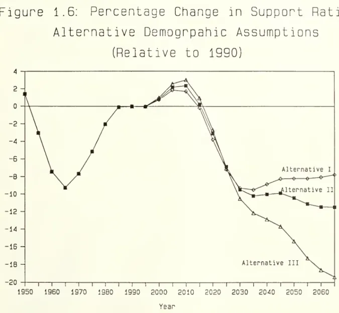
Finally, while the decline in the support ratio by the middle of the next

century is large, there is still substantial uncertainty about the ultimate

burden. Figure 1.6 presents support ratios using LF2 and C0N2, under the

Figure

1.6:

Percentage

Change

in

Support

Ratio,

Alternative

Demogrpahic

Assumptions

-

(Relative

_to

₁₉₉₀₎

o

en en > oi X cu c -2 --4 --5 -8 -10 12 14 --16 -18 _H -20 Alternative I -©

—

—

^

Alternative III I \ I I 1 I I I I I I I I I 1 I I I 1 1 I I 1950 1960 1970 1980 1990 2000 2010 2020 2030 2040 2050 2060 Year

Note: The Figure shows the Support Ratio under three demographic assumptions.

15

substantial differences between the scenarios, particularly between the more

pessimistic Case III scenario and the Case lib scenario which is our standard

case. The decline in the support ratio is almost twice as large in the

pessimistic scenario as in our benchmark. Even in the optimistic Case I

scenario, the support ratio still declines by almost eight percent between

16

2. Capital Accumulation and Shifting Dependency Burdens

This section explores how the demographic shifts described above affect

the economy's sustainable level of consumption, and how society should plan

for these changes. We find that sustainable consumption increases for the

next several decades , and that an economy with otherwise-optimal national

saving would reduce its saving in response to the coming demographic changes.

2.1 Steady State Consumption Opportunities

Demographic change has two effects on consumption opportunities. First,

an increase in dependency lowers output per person, thus reducing consumption

per capita. Second, slower labor force growth reduces investment

requirements, thus reducing the need for saving and increasing consumption per

capita.

To examine the importance of these two changes for consumption

opportunities, we assume that output per worker, f (k) , is divided between

consumption and investment. Maintaining constant capital intensity requires

investment of n*k, where n is the labor force growth rate , k is the

capital-labor ratio, and for expositional ease, we have assumed away depreciation and

technical change. When the labor force and the population are not the same,

consumption per capita is only a fraction of output net of investment per

worker. This fraction is the ratio of the number of workers to the size of

12

A substantial part of the U.S. capital stock is residential capital.

The natural steady-state condition for housing requires investment at the rate

of population growth, not the rate of labor force growth. In steady state,

these two growth rates will coincide.

13_We

17

the population, precisely the support ratio (a) defined above. The resulting

equation for per capita consumption is:

(2.1) c = Q[f(k) - k*n]

.

This expression can be rewritten to find the change in steady— state

consumption for changes in a and n:

(2.2) Ac/c = Aa/a - [Q*(k/c)*An + (k/c)*AQ*An]

with c, k, and a evaluated at the initial steady state. Equation (2.2)

illustrates the two steady— state effects of demographic change. A decline in

the labor force—to—population ratio (a) reduces the level of per capita

consumption which is feasible given the economy's capital stock. At the same

time, a decline in the growth rate of the labor force (n) permits more

consumption for a given capital— output ratio. Society receives a consumption

dividend when it is able to invest less and still maintain a given level of

per capita output. This "Solow effect" offsets the long run dependency effect

on per capita consumption.

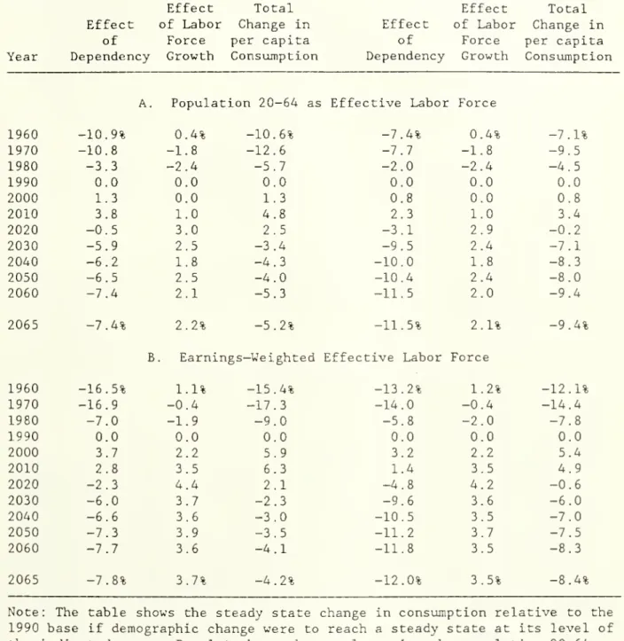
Table 2.1 reports the magnitude of these two effects. For each year, we

show the steady-state consumption change associated with changes in a (the

first column) , n (the second column) , and the combined effect (the third

column) . The components due to the dependency increase are the same as those

in Section 1; the other columns show the extent to which changing investment

needs offset this effect.

Two results emerge from Table 2.1. First, the consumption benefits from

reduced investment requirements are substantial. During the next two decades.

We have arbitrarily assigned the second-order term to the second effect

in our decomposition. We have also assumed that the capital-labor ratio, and

thus the capital—consumption ratio do not change with demographic change. The

Table 2.1: Shifting Steady-State Per Capita Consumption

Needs: Total Population

Effect Total

Effect of Labor Change in

of Force per capita

Year Dependency Growth Consumption

Equivalence Scale

Effect Total

Effect of Labor Change in

of Force per capita

Dependency Growth Consumption

A. Population 20-64 as Effective Labor Force

1960 1970 -10.9% -10.8 0.4% -1.8 -10.6% -12.6 -7.4% 0.4% -7.1% 1980 -3.3 -2.4 -5.7 1990 0.0 0.0 0.0 2000 1.3 0.0 1.3 2010 3.8 1.0 4.8 2020 -0.5 3.0 2.5 2030 -5.9 2.5 -3.4 2040 -6.2 1.8 -4.3 2050 -6.5 2.5 -4.0 2060 -7.4 2.1 -5.3 -7.7 -1.8 -9.5 -2.0 -2.4 -4.5 0.0 0.0 0.0 0.8 0.0 0.8 2.3 1.0 3.4 -3.1 2.9 -0.2 -9.5 2.4 -7.1 10.0 1.8 -8.3 •10.4 2.4 -8.0 11.5 2.0 -9.4 2065 -7.4% 2.2% -5.2% -11.5% 2.1% -9.4%

B. Earnings-Weighted Effective Labor Force

1960 -16.5% 1.1% -15.4% -13.2% 1.2% -12.1% 1970 -16.9 -0.4 -17.3 -14.0 -0.4 -14.4 1980 -7.0 -1.9 -9.0 -5.8 -2.0 -7.8 1990 0.0 0.0 0.0 0.0 0.0 0.0 2000 3.7 2.2 5.9 3.2 2.2 5.4 2010 2.8 3.5 6.3 1.4 3.5 4.9 2020 -2.3 4.4 2.1 -4.8 4.2 -0.6 2030 -6.0 3.7 -2.3 -9.6 3.6 -6.0 2040 -6.6 3.6 -3.0 -10.5 3.5 -7.0 2050 -7.3 3.9 -3.5 -11.2 3.7 -7.5 2060 -7.7 3.6 -4.1 -11.8 3.5 -8.3 2065 -7.8% 3.7% -4.2% -12.0% 3.5% -8.4%

Note: The table shows the steady state change in consumption relative to the

1990 base if demographic change were to reach a steady state at its level of

the indicated year. Panel A shows the results using the population 20-64

(LFl) as the effective labor force. Panel B shows the results using

18

the benefits of slower labor force growth will be about 1 to 3.5 percent of

per capita consumption, using the 1990 base. Since the labor force was

growing more rapidly in the 1970s and 1980s than in 1990, the effect of

reduced investment requirements is even larger relative to earlier years. By

the middle of the next century, the benefits of slower labor force growth will

be between 2.1 and 3.7 percent of per capita consumption. This is between

one— quarter and one—half of the adverse dependency effects of the changing

population mix.

Second, while the investment effect offsets a substantial part of the

long term dependency increase, it magnifies the short run effect of rising

support ratios. Reduced dependency and slowing labor force growth both

increase consumption possibilities so that by 2010, society will be between 3

and 6% richer, depending on the combination of labor force and needs measures.

Only after 2020 does the increase in dependency outweigh the decline in

investment needs and reduce consumption below its 1990 level.

The steady state consumption decline between 1990 and 2060 is estimated

at between 4% (with effective consumers set equal to total population) and 9%

(with effective consumers computed using equivalence scales) . As with the

support ratios, this finding is more sensitive to our definition of

consumption needs than to our choice regarding the definition of the effective

labor force. For almost all cases, however, society is richer in the new

steady state than in 1970 or 1980.

2.2 Demographic Change and Optimal Capital Accumulation

The results presented so far suggest that in the short run, demographic

19

maintaining the level of capital intensity. In the long run, they will reduce

the sustainable level of consumption. The question then becomes how society

should adjust its saving policy to these developments. In order to study this

question, we use the standard Ramsey optimal growth model.

We assume that a social planner seeks to maximize

(2.3) V = _{j^ e-^^*P(t)*U(c^)} dt

where P(t) denotes the number of individuals alive in period t, c(t) is per

capita consumption, and p is the social time preference rate. We denote the

current period as time zero. This social welfare function weights the utility

of a representative individual in each generation by the generation's size.

In our earlier notation, P(t) = N(t)/Q:^^ where N(t) is the labor force and _q^^

is the support ratio.

Our analysis abstracts from the overlapping generations structure of the

actual population. Calvo and Obstfeld (1988) formally justify this procedure

by demonstrating that if age-specific transfer programs like Social Security

are available, and if individual utility functions are additively separable,

then "the Cass-Koopmans-Ramsey framework can be used to evaluate paths of

aggregate consumption in models where different generations co-exist...the

planning problem facing the government can be decomposed into two

sub-problems: a standard problem of optimal aggregate capital accumulation, and a

Some might argue for using an alternative objective function which does

not weight the average utility of different generations by the number of

people in the generation. This will lead the social planner to raise average

consumption in small cohorts relative to that in larger cohorts, because the

aggregate resource cost of raising the average consumption of persons in small

cohorts is less than that for large cohorts. We see no legitimate ethical

20

problem of distributing consumption optimally on each date among generations

alive then (p. 163) .

"

The social planner maximizes (2.3) subject to a capital accumulation

constraint analogous to equation (2.1):

(2.4) k^ = f(k^) - c^/Q^ - k^*n^.

If a^ = 1, equation (2.4) reduces to the standard resource constraint in

neoclassical growth models. The consumption profile which solves this problem

satisfies:

(2.5) c^/c^ = a*[f'(k^) - _p]

where a = -U' (Cj^)/c^*U"(c^^) , the elasticity of substitution in consumption.

In steady state with no technical progress, per capita consumption and

the capital— labor ratio must be constant. From the Euler equation (2.5), we

find that constant consumption requires

(2.6) k* = f'-^[p].

This locus, a vertical line in (c,k) space, is drawn in Figure 2.1. Constancy

of the capital-labor ratio given in equation (2.1) yields the second locus

drawn in Figure 2.1.

Permanent reductions in q, the support ratio, scale back the feasible

level of per capita consumption for each k, shifting the k = locus as shown

in Figure 2.2. The steady-state capital-labor ratio is unaffected by this

change, so the only effect of this shock is an immediate and permanent decline

in consumption per capita. Reductions in n, the labor force growth rate, have

the opposite effect, shifting the k = frontier out. The steady-state

consumption effect of a demographic shift such as a fertility decline, which

The optimal plan must also satisfy transversality conditions noted for

Figure

2.1:

Steady-state

Analysis

of

Optimal

Consumption

Level

C »0

c

21

reduces both a and n, depends on which of these effects is larger. Reductions

in n unambiguously reduce the optimal steady state saving rate while increases

in a have no effect on steady state savings.

The actual demographic projections for the United States are more complex

than an immediate shift in either q or n, however. For the next several

decades, the net effect of demographic change is an outward shift in the k =

locus, followed by a period of inward shift which terminates with the locus

below its current level. When consumers have perfect foresight and recognize

the complex nature of the demographic transition, the initial consumption

response to news of the demographic transition is theoretically ambiguous.

Figures 2.3a and 2.3b illustrate this. Each presents a scenario in which the k

= frontier shifts out and then back. In the first case consumption

increases when demographic news arrives, while in the second consumption

initially declines.

This ambiguity suggests the need for explicit numerical simulations to

address the optimal consumption response. We assume that the utility function

in (2.3) has the form

(2.7) U(c^) = (c^l-V'^ _ _l)/(l-l/a)

where a is the elasticity of substitution in consumption. We also assume a

constant elasticity of substitution production function:

(2.8) f(k^.) = [a*k^^/^-^ + b]^--^.

The elasticity of substitution in production is fi. To find the transition path

between one steady state and another, we discretize differential equations

This is easily seen from the Harrod-Domar condition k/f(k) = s/n, where

s is the saving rate out of national income, and the observation that neither

changes in a nor changes in n affect optimal steady state capital intensity in

Figure

_2.3:

_Optimal

_Consumption

Response

to

a

Fertility

_Decline

c«o ^^OAiwM»»fn»<\ (_a^ Cor.io^p+-von 3w"*<>» Wp

\

C»^it-«-i I iJocU.«r

22

(2.4) and (2.5) and employ a grid-search algorithm to find the initial

"1₈

consumption level which will lead the economy to the new steady state.

Our simulations also allow for labor augmenting technical change (g) and

depreciation (5), which are introduced into equations (2.4) and (2.5) in the

standard way . Although consumption grows over time when there is technical

progress, the consumption numbers we report are relative to the consumption

that would have been possible without demographic change. We assume that

technical change is equal to 1.4 percent per year, the Social Security

Administration's steady-state projection. The depreciation rate is set

equal to 4.09 percent, the US average from 1952-1987. Finally, we use data

for this period on payments to labor and capital to estimate capital's share

in gross output

—

33.2 percent. These two numbers imply a steady state

marginal product of capital of 14.4 percent. From equation (2.5), this

implies an effective discount rate (p + a*g) of 10.3 percent.

18

Since the Social Security Administration only forecasts population in

every fifth year, we interpolate annual observations using a smooth

interpolator. The results are not sensitive to the frequency of the data.

19

Following Blanchard and Fischer (1989), we express capital per

"effective worker", where effective workers grow at n+g. Consumption is

expressed per "effective person". In equation (2.5), the effective discount

rate becomes (p + S + g*a)

.

20

Our results are insensitive to the choice of g.

21

Our depreciation rate is estimated as capital consumption allowances

divided by the aggregate capital stock. We define aggregate capital as

national assets minus consumer durables minus one half of the value of land.

Consumer durables are excluded since they are not included in output. One

half of land is included in capital to allow for natural resource values to

change

.

22

Capital's share in output is total output less wages and salaries,

two-thirds of proprietors income (the estimated labor compensation) and indirect

23

We present results using two values of a, a benchmark case of unit

elasticity (c-l) and an alternative elasticity of substitution of one-tenth

(a=.l). We also choose two values for the elasticity of substitution in

production, a benchmark of unit elasticity (^"=1) and an alternative elasticity

of one-half (/9-=.5). When the elasticity of substitution in consumption is

low, consumption today is not a good substitute for consumption tomorrow, and

we expect more consumption smoothing. When the elasticity of substitution in

production is low, saving does not get a high return since the extra capital

does not substitute well for the smaller labor force, and we expect less

consumption smoothing.

Demographic change has occurred gradually over the last 25 years, as the

baby boom has given way to the baby bust. It is not obvious how best to model

these changes as a single shock. Initially, we assume the economy is in

steady state with values of a and n corresponding to those prevailing in 1990,

and ask how consumption and saving should evolve henceforth. Since some of

the consequences of demographic change were already known by 1990, we go on to

examine how consumption and saving should have responded in 1970 and 1980 if

news of demographic change suddenly arrived.

For all our simulations, we use the trajectories of q and n implied by

the Social Security Administration's lib forecasts, and further assume that

the predicted values for 2065 persist as the economy's final steady state.

The resulting consumption changes are thus the optimal response to the

demographic transition which the U.S. will undergo over the next seven

decades, assuming these changes were unforeseen as of 1990.

The results of these simulations are shown in Table 2.2. The level of

Table 2.2: Optimal Consumption Response to Demographic Shocks

Substitution Elasticity in Production: 1.0

Substitution Elasticity in Consumption: 1.0

1.0 0.1 0.5 1.0 0.5 0.1

Expectations: Static Perfect Foresight

Case 1: Labor Force=Population 20—64: Effective Consumers—Total Population

Initial Steady State 100.0

Adjustment 100.0 Time Path 2000 101.3 2010 104.8 2020 102.5 2030 96.6 2040 95.7 2050 96.0 2060 94.7 00.0 100.0 100.0 100.0 00.6 101.1 100.4 101.0 01.4 101.3 101.4 101.3 03.3 101.7 103.8 102.1 02.3 101.4 102.5 101.7 98.3 100.3 97.7 99.8 96.2 99.0 95.9 98.1 95.9 98.1 95.9 97.1 95.1 97.3 95.0 96.2

New Steady State 94.8 94.8 94.8 94.8 94.8

Case 2: Lablor :Force=Earninps-•Weighted; Effective Consumers-=Equival ence Scale

Initial Steady State 100.0 100.0 100.0 100.0 100.0

Initial Adiustment 100.0 102.3 102.8 101.9 102.8

Time Pa th 2000 105.4 104.1 103.0 104.5 103.3 2010 104.9 104.1 102.8 104.5 103.0 2020 99.4 100.4 101.5 100.2 101.1 2030 94.0 95.7 99.6 95.0 98.3 2040 93.0 93.5 97.8 93.2 96.0 2050 92.5 92.7 96.3 92.6 94.5 2060 91.7 92.0 95.1 91.8 93.4

New Ste.ady State 91.6 91.6 91.6 91.6 91.6

Note: Each column is the simulated path of consumption in response to a

demographic shock like that which the U.S. will experience between 1990 and

2060. The static expectations column is the change in consumption assuming

that agents in each period assume that the current level of a and n will

persist forever. The "perfect foresight" columns assume current knowledge of

the entire path of demographic change. The initial steady state is the 1990

24

first column in Table 2.2, the static expectations response, is the change in

consumption if consumers have no foresight about demographic change, but

rather assume at each date that current conditions will pesist forever. It

thus corresponds to the consumption path in Table 2.1. The other four columns

assume that consumers in 1990 have perfect foresight regarding future

demographic changes.

For all of the parameter values, consumption rises initially in response

to the demographic transition, by up to 2.2 percent relative to the steady

state implied by 1990 demography. This result is insensitive to the parameter

choices we present. Consumption remains above its 1990 level until 2020 or

later. Thus, demographic shifts during the next half century optimally raise

present consumption. The effect is more pronounced when consumption is less

substitutable over time and less pronounced when production is less

substitutable over time.

Figure 2.A shows the movements of consumption and capital for the

simulations using the Case 2 assumptions and the unit elasticities of

substitution in production and consumption are shown in Figure 2.4. The

corresponding saving rate is shown in Figure 2.5. Consumption initially rises

by 2. 3 percent. This is followed by a period of declining capital-labor

ratios, during which consumption continues to increase. The shifting

opportunity locus due to the decline in labor force growth ultimately causes

an increase in saving and thus in capital intensity, even at the higher level

of consumption. After the period of capital deepening, consumption begins to

23

In addition to the parameter values reported, we have experimented with

elasticities in substitution and production up to 10. For none of these cases

is there an initial increase in savings

Figure

2.4:

Optimal

Consumption

and

Capital-Labor

Paths

Following

Demographic

Change

c o m L. 0} D. > u CD c o en c a 105 104

_H

103 102 101 -100 -99 98

H

97 96 -95 -94 93 92 -91 266 ?ee& Initial Steady State 20r0 202^1 2050 5060

view Steady State

270 274 278 282 286 290

Capital per Effective Worker

Note: The Figure shows the trajectory of consumption per effective person

and capital per effective worker for the simulation using the LF2 and C0N2 measures of labor force and needs.

7 6.5 6 -5.5 -5 -ID QC in en 4.5 -c r1 > (tJ

4-3.5

-

3-2.5

Figure

2.5:

Optimal

Saving

Rates

in

Response

to

Demographic

Change

2 I I I I I I I I I I I I I I M I I I I I I I I I I I I I I I I I I I I I I I I I I I I I I I I I I I I I I I1 I I I I I I I I I I I I I I I I I I I I I I I I I I

1990 1995 2000 2005 2010 2015 2020 2025 2030 2035 2040 2045 2050 2055 2060 2065 2070

YEAR

Note: The Figure shows the optimal saving path for the simulation

25

decline. Finally, when the increase in dependency overtakes the favorable

effects of the slowing labor force growth, both consumption and capital

decline to the new steady state, and saving falls.

As Figure 2.5 demonstrates, the saving rate initially falls by almost 2

percentage points. The saving rate then increases for a few years, though it

never attains its initial steady state value. This increase is due to the

increase in the support ratio, which allows both consumption per person and

the saving rate to increase. Finally, the saving rate begins to fall towards

its new long run level, equal to the amount of saving necessary to equip the

more slowly growing labor force.

We also ran the simulations using the Case I and Case III Social Security

alternatives, with no substantive changes in results. Consumption rises less

with the Case I assumptions than with our benchmark Case lib assumptions,

since the number of dependent children does not decrease as quickly, and more

with the Case III assumptions, where there is an even larger short run

benefit. In ass three cases the response to the demographic news is a

decrease in saving. We have also experimented with changing capital's share

or the assumed initial level of capital intensity in order to vary the

/

discount rate p. Even with a pure discount rate as low as zero, our

conclusion that consumption rises following a demographic shock remains valid.

/

Since the effective discount rate must equal the marginal product of

capital in steady state, and the marginal product of capital is the ratio of

capital's share in output to the capital-output ratio, changes in the

effective discount rate have to be accompanied by changes in either capital's

26

Finally, we explored how consumption would change if we began the

simulations in 1970 or 1980. As Table 2.1 demonstrated, consumption

possibilities are higher in 1990 than in any of the three previous decades.

Figure 2.6 shows the deviation of the saving rate from its initial steady

state level after the demographic news. In all of the simulations, saving

falls immediately following the demographic news, and is always falling by

2000. Even in the cases where saving begins to increase in the 1990's

—

when

we begin the simulation in 1980 or 1990

—

the saving rate is lower throughout

the 1990's than the original steady state, and it begins a period of prolonged

decline by 2000. While these figures help to develop perspective on the

recent decline in U.S. saving and investment rates, the actual decline in U.S.

national saving from an average of 7.1 percent in the 1970s to about 2 percent

in the late 1980s is considerably more than our demographic analysis can

justify.

The analysis in this section reaches a clear conclusion. For an economy

choosing its consumption path in accord with a standard optimal growth model,

the right response to the upcoming U.S. demographic change would be an

increase in consumption and a reduction in national saving. For all plausible

combinations of parameter values, the effects of reduced labor force growth

and reductions in the number of children exceed the effects of increases in

en en o ro (X en c f-i > en u c lU cu

Figure

2.6:

Change

in

Saving

Rates

in

Response

to

Demognaphic

Change,

Using

Different

Beginning

Dates

-i --2 --4 --5 ^ Starting in 1970 1/ 1/ Starting in 1980\ \ 1111111 11 111111 111111 111 111 111111111111 111111111 111111111 111 11111 111111 111111111111 111111111111111 111 1 1970 1980 1990 2000 2010 2020 2030 2040 2050 2060 2070 YEAR

Note: The Figure shows the percentage point difference in saving

rates from the initial steady state following a demographic change. All three simulations use the LF2 and C0N2 measures of labor

27

3. Open Economy Aspects of the Demopraphlc Shift

Our analysis thus far has focused on the demographic change in the United

States. When capital markets are integrated, however, the demographic shift

in the U.S. must be measured not only in absolute terms but relative to the

coincident shifts in our major trading partners. This section compares the

degree of population aging in different nations, and extends our earlier

simulation model to consider the U.S. in relation to other OECD countries.

Our earlier finding that, ceteris paribus, demographic changes justify a

reduction in optimal saving is reinforced when we allow for international

capital flows, since demographic change is less pronounced in the U.S. than

elsewhere in the OECD.

]

3.1 Relative Rates of Population Aging

To compare rates of population aging, we use projections by the OECD

(1988). These projections differ in two important ways from the Social

Security Administration projections used above for the U.S. First, the OECD

treats the 15-19 age group as workers rather than dependents. Second, and

more important, the OECD assumes that fertility rates in all countries will

converge to the replacement level of 2.1 by 2050. Since U.S. fertility rates

are currently well above those in most of the OECD, this understates the

likely contrast between the future U.S. and foreign demographic experiences.

Figure 3.1 shows the historical and projected elderly dependency ratio

for the U.S., Japan, and the European Community. The elderly dependency

ratio increases substantially in all countries, with the most rapid increase

25_The

multi-country index is a GDP-weighted average of the indices for

Figure

3.1:

Elderly

Dependency

Ratios,

1950-2050,

U.S.,

Japan,

and

European

Community

u CD Q. ^d -40 -

^.

38

-X

/--^^^

36

-/

/

34 -

*^/

/

32 - Japan /'^

/^

" _-— ^ 30 -

_/

y

/

28 - 1

/

X

/

26 -

/

y^^

/

24 -22 - EC

/

20

-^X^^,^^

—

,/ _

-*

U.S. IB -

wy.

^

16 -

^

'*^^^^*^^

^

/

14^

^/^^

y^^^^^

12-^

/^^

10 -u

—

R — r D 1 1 1 1 1 1 1 1 1 1950 1970 1990 2010 2030 2050 Year

Note: The Figure shows the ratio of the elderly population to the

population 15-64.

28

in Japan. By 2050, even with a 19 percentage point increase in the elderly

dependency ratio, the United States' ratio will be roughly 5 percentage points

lower than in the other countries.

Figure 3.2 shows the path of the support ratio corresponding to the LFl

and CONl assumptions earlier. The broad outlines for all three regions are

similar. All have higher support ratios in 1990 than in 1960, and all will

have much lower support ratios by the middle of the next century than they do

today. The ultimate level of United States dependency will be lower than that

abroad.

Two differences in these indices are notable, however. First, the United

States will be better off for the next two decades than it is now, while the

other countries experience declines in the support ratio beginning in 1990.

Second, the U.S. and EC dependency ratios are driven principally by fertility

changes, while the Japanese changes are driven to a much larger extent by

reductions in mortality. The decline in the support ratio in the 1950s in the

United States and in the 1960's in the EC is due to increased numbers of

children; the rise in the support ratio throughout the post-war period in

Japan, in contrast, is caused by reduced mortality at middle and older ages.

Since the labor force grows faster when fertility is higher, the reduction in

labor force growth over the next several decades , and thus the consumption

dividend from reduced investment requirements, will be larger in the U.S. and

the European Community than in Japan.

To evaluate the size of the demographic transition abroad. Table 3.1

reports the optimal consumption and saving responses to projected demographic

Figure

3.2;

Support

Ratios.

1950-2050.

II

o

Ol CD o a. a. cn

U.S.,

Japan,

and

European

Community

1970 1990 2010 2030 2050

Year

Table 3.1: Autarky Response of Consumption and Saving to Demographic Shocks US Japan Country European Cominunity Non-US OECD Total OECD A. Consumption Response Initial Steady State Adjustment Time Path 2000 2010 2020 2030 2040 2050 100,.0 100..1 100,.6 101,.5 99,.1 94,.4 92,.0 92,.1 100.0 99.2 97, 92, 89.0 88.5 86.3 84.8 100.0 100.1 99.7 98.8 97.1 92.8 89.1 88.2 100,.0 100,,0 99,.3 97,.8 95,.5 92,.1 87.9 100.0 100.1 99.8 99.2 97.0 93.0 89.9 89.1 New Steady State 92.3 84.4 87.9 87.8 89.0

B. Saving Rate Response

Adjustment -0.10 0.72 -0.12 0.02 -0.04 Time PsLth 2000 0.14 -1.36 -0.88 -0.95 -0.60 2010 0.47 -3.03 -0.69 -1.14 -0.52 2020 -1.44 -2.63 -1.46 -1.80 -1.58 2030 -2.44 -1.30 -2.76 -2.51 -2.54 2040 -1.51 -3.08 -2.89 -2.90 -2.30 2050 -1.36 -1.48 -0.84 -1.20 -1.32 New Steady State -1.51 -1.28 -0.69 -1.09 -1.25

Note: The values in the table are the optimal consumption and saving paths for

each country without international capital flows. We use the equivalence

scale for consumption needs. Consumption is relative to the initial steady

state, which is assumed to be 100. Savings paths are defined as the

percentage point difference between the saving rate along the path and the

initial steady state. The elasticities of substitution in production and

29

OECD. These consumption paths are simulated using the model of the last

section. For the United States, consumption rises only slightly initially,

continues increasing until 2010, and then declines to the new steady state.

This consumption increase is accompanied by an increased saving rate, however,

since the relative increase in the working age population increases output per

person by more than consumption per person.

For Japan, the coming demographic changes reduce optimal consumption

initially by just under 1 percent, and consumption continues to decline

throughout the next 60 years, even as the saving rate declines. For the

European Community, there is also a slight increase in consumption, but by

2000 consumption is lower, and continues to decline throughout the next half

century. This pattern of declining consumption after a small increase in

initial consumption carries over to the non-U.S. OECD and total OECD

simulations

.

The initial decrease in the saving rate in the United States, and the

increase in the non—U.S. OECD implies that in an open economy capital would

initially flow from the non-U.S. OECD to the United States. After the initial

change in saving, however, capital flows are more difficult to predict. In

addition to the change in saving rates in the autarky case, the countries also

have different changes in labor force growth rates and thus investment

requirements. Since the desired capital inflow depends on the difference

96

The table uses the case of unit elasticities of substitution and

production. We assume that depreciation rates and rates of labor augmenting

technical progress are equal in all countries and are the same as the Social

Security Administration forecasts for the U.S.. The assumption of equal

productivity growth is obviously wrong but probably does not have a large

impact on estimates of the change in saving due to changes in demographic

structure