HAL Id: hal-00935640
https://hal.inria.fr/hal-00935640v2
Submitted on 29 Nov 2014
HAL is a multi-disciplinary open access
archive for the deposit and dissemination of
sci-entific research documents, whether they are
pub-lished or not. The documents may come from
teaching and research institutions in France or
abroad, or from public or private research centers.
L’archive ouverte pluridisciplinaire HAL, est
destinée au dépôt et à la diffusion de documents
scientifiques de niveau recherche, publiés ou non,
émanant des établissements d’enseignement et de
recherche français ou étrangers, des laboratoires
publics ou privés.
Benchmark (BRATS)
Bjoern Menze, Andras Jakab, Stefan Bauer, Jayashree Kalpathy-Cramer,
Keyvan Farahani, Justin Kirby, Yuliya Burren, Nicole Porz, Johannes
Slotboom, Roland Wiest, et al.
To cite this version:
Bjoern Menze, Andras Jakab, Stefan Bauer, Jayashree Kalpathy-Cramer, Keyvan Farahani, et al..
The Multimodal Brain Tumor Image Segmentation Benchmark (BRATS). IEEE Transactions on
Medical Imaging, Institute of Electrical and Electronics Engineers, 2014, 34 (10), pp.1993-2024.
�10.1109/TMI.2014.2377694�. �hal-00935640v2�
The Multimodal Brain Tumor
Image Segmentation Benchmark (BRATS)
Bjoern H. Menze
∗†, Andras Jakab
†, Stefan Bauer
†, Jayashree Kalpathy-Cramer
†, Keyvan Farahani
†, Justin Kirby
†,
Yuliya Burren
†, Nicole Porz
†, Johannes Slotboom
†, Roland Wiest
†, Levente Lanczi
†, Elizabeth Gerstner
†,
Marc-Andr´e Weber
†, Tal Arbel, Brian B. Avants, Nicholas Ayache, Patricia Buendia, D. Louis Collins,
Nicolas Cordier, Jason J. Corso, Antonio Criminisi, Tilak Das, Herv´e Delingette, C
¸ a˘gatay Demiralp,
Christopher R. Durst, Michel Dojat, Senan Doyle, Joana Festa, Florence Forbes, Ezequiel Geremia, Ben Glocker,
Polina Golland, Xiaotao Guo, Andac Hamamci, Khan M. Iftekharuddin, Raj Jena, Nigel M. John,
Ender Konukoglu, Danial Lashkari, Jos´e Ant´onio Mariz, Raphael Meier, S´ergio Pereira, Doina Precup,
Stephen J. Price, Tammy Riklin Raviv, Syed M. S. Reza, Michael Ryan, Duygu Sarikaya, Lawrence Schwartz,
Hoo-Chang Shin, Jamie Shotton, Carlos A. Silva, Nuno Sousa, Nagesh K. Subbanna, Gabor Szekely,
Thomas J. Taylor, Owen M. Thomas, Nicholas J. Tustison, Gozde Unal, Flor Vasseur, Max Wintermark,
Dong Hye Ye, Liang Zhao, Binsheng Zhao, Darko Zikic, Marcel Prastawa
†, Mauricio Reyes
†‡,
Koen Van Leemput
†‡B. H. Menze is with the Institute for Advanced Study and Department of Computer Science, Technische Universit¨at M¨unchen, Munich, Germany; the Computer Vision Laboratory, ETH, Z¨urich, Switzerland; the Asclepios Project, Inria, Sophia-Antipolis, France; and the Computer Science and Artificial Intelligence Laboratory, Massachusetts Institute of Technology, Cambridge MA, USA.
A. Jakab is with the Computer Vision Laboratory, ETH, Z¨urich, Switzer-land, and also with the University of Debrecen, Debrecen, Hungary.
S. Bauer is with the Institute for Surgical Technology and Biomechanics, University of Bern, Switzerland, and also with the Support Center for Advanced Neuroimaging (SCAN), Institute for Diagnostic and Interventional Neuroradiology, Inselspital, Bern University Hospital, Switzerland.
J. Kalpathy-Cramer is with the Department of Radiology, Massachusetts General Hospital, Harvard Medical School, Boston MA, USA.
K. Farahani and J. Kirby are with the Cancer Imaging Program, National Cancer Institute, National Institutes of Health, Bethesda MD, USA.
R. Wiest, Y. Burren, N. Porz and J. Slotboom are with the Support Center for Advanced Neuroimaging (SCAN), Institute for Diagnostic and Interven-tional Neuroradiology, Inselspital, Bern University Hospital, Switzerland.
L. Lanczi is with University of Debrecen, Debrecen, Hungary.
E. Gerstner is with the Department of Neuro-oncology, Massachusetts General Hosptial, Harvard Medical School, Boston MA, USA.
B. Glocker is with BioMedIA Group, Imperial College, London, UK. T. Arbel and N. K. Subbanna are with the Centre for Intelligent Machines, McGill University, Canada.
B. B. Avants is with the Penn Image Computing and Science Lab, Department of Radiology, University of Pennsylvania, Philadelphia PA, USA. N. Ayache, N. Cordier, H. Delingette, and E. Geremia are with the Asclepios Project, Inria, Sophia-Antipolis, France.
P. Buendia, M. Ryan, and T. J. Taylor are with the INFOTECH Soft, Inc., Miami FL, USA.
D. L. Collins is with the McConnell Brain Imaging Centre, McGill University, Canada.
J. J. Corso, D. Sarikaya, and L. Zhao are with the Computer Science and Engineering, SUNY, Buffalo NY, USA.
A. Criminisi, J. Shotton, and D. Zikic are with Microsoft Research Cambridge, UK.
T. Das, R. Jena, S. J. Price, and O. M. Thomas are with the Cambridge University Hospitals, Cambridge, UK.
C. Demiralp is with the Computer Science Department, Stanford University, Stanford CA, USA.
S. Doyle, F. Vasseur, M. Dojat, and F. Forbes are with the INRIA Rhˆone-Alpes, Grenoble, France, and also with the INSERM, U836, Grenoble, France. C. R. Durst, N. J. Tustison, and M. Wintermark are with the Department of Radiology and Medical Imaging, University of Virginia, Charlottesville VA, USA.
J. Festa, S. Pereira, and C. A. Silva are with the Department of Electronics, University Minho, Portugal.
P. Golland and D. Lashkari are with the Computer Science and Artificial Intelligence Laboratory, Massachusetts Institute of Technology, Cambridge MA, USA.
X. Guo, L. Schwartz, B. Zhao are with Department of Radiology, Columbia University, New York NY, USA.
A. Hamamci and G. Unal are with the Faculty of Engineering and Natural Sciences, Sabanci University, Istanbul, Turkey.
K. M. Iftekharuddin and S. M. S. Reza are with the Vision Lab, Department of Electrical and Computer Engineering, Old Dominion University, Norfolk VA, USA.
N. M. John is with INFOTECH Soft, Inc., Miami FL, USA, and also with the Department of Electrical and Computer Engineering, University of Miami, Coral Gables FL, USA.
E. Konukoglu is with Athinoula A. Martinos Center for Biomedical Imag-ing, Massachusetts General Hospital and Harvard Medical School, Boston MA, USA.
J. A. Mariz and N. Sousa are with the Life and Health Science Research Institute (ICVS), School of Health Sciences, University of Minho, Braga, Portugal, and also with the ICVS/3B’s - PT Government Associate Laboratory, Braga/Guimaraes, Portugal.
R. Meier and M. Reyes are with the Institute for Surgical Technology and Biomechanics, University of Bern, Switzerland.
D. Precup is with the School of Computer Science, McGill University, Canada.
T. Riklin Raviv is with the Computer Science and Artificial Intelligence Laboratory, Massachusetts Institute of Technology, Cambridge MA, USA; the Radiology, Brigham and Women’s Hospital, Harvard Medical School, Boston MA, USA; and also with the Electrical and Computer Engineering Department, Ben-Gurion University, Beer-Sheva, Israel.
H.-C. Shin is from Sutton, UK.
G. Szekely is with the Computer Vision Laboratory, ETH, Z¨urich, Switzer-land.
M.-A. Weber is with Diagnostic and Interventional Radiology, University Hospital, Heidelberg, Germany.
D. H. Ye is with the Electrical and Computer Engineering, Purdue Univer-sity, USA.
M. Prastawa is with the GE Global Research, Niskayuna NY, USA. K. Van Leemput is with the Department of Radiology, Massachusetts General Hospital, Harvard Medical School, Boston MA, USA; the Technical University of Denmark, Denmark; and also with Aalto University, Finland.
†These authors co-organized the benchmark; all others contributed results
of their algorithms as indicated in the appendix.
‡These authors contributed equally.
∗To whom correspondence should be addressed
Abstract—In this paper we report the set-up and results of the Multimodal Brain Tumor Image Segmentation Benchmark (BRATS) organized in conjunction with the MICCAI 2012 and 2013 conferences. Twenty state-of-the-art tumor segmentation algorithms were applied to a set of 65 multi-contrast MR scans of low- and high-grade glioma patients – manually annotated by up to four raters – and to 65 comparable scans generated using tumor image simulation software. Quantitative evaluations revealed considerable disagreement between the human raters in segmenting various tumor sub-regions (Dice scores in the range 74-85%), illustrating the difficulty of this task. We found that different algorithms worked best for different sub-regions (reaching performance comparable to human inter-rater variabil-ity), but that no single algorithm ranked in the top for all sub-regions simultaneously. Fusing several good algorithms using a hierarchical majority vote yielded segmentations that consistently ranked above all individual algorithms, indicating remaining opportunities for further methodological improvements. The BRATS image data and manual annotations continue to be publicly available through an online evaluation system as an ongoing benchmarking resource.
I. INTRODUCTION
G
LIOMAS are the most frequent primary brain tumorsin adults, presumably originating from glial cells and infiltrating the surrounding tissues [1]. Despite considerable advances in glioma research, patient diagnosis remains poor. The clinical population with the more aggressive form of the disease, classified as high-grade gliomas, have a median survival rate of two years or less and require immediate treatment [2], [3]. The slower growing low-grade variants, such as low-grade astrocytomas or oligodendrogliomas, come with a life expectancy of several years so aggressive treatment is often delayed as long as possible. For both groups, intensive neuroimaging protocols are used before and after treatment to evaluate the progression of the disease and the success of a chosen treatment strategy. In current clinical routine, as well as in clinical studies, the resulting images are evaluated either based on qualitative criteria only (indicating, for example, the presence of characteristic hyper-intense tissue appearance in contrast-enhanced T1-weighted MRI), or by relying on such rudimentary quantitative measures as the largest diameter visible from axial images of the lesion [4], [5].
By replacing the current basic assessments with highly accurate and reproducible measurements of the relevant tumor substructures, image processing routines that can
automat-ically analyze brain tumor scans would be of enormous
potential value for improved diagnosis, treatment planning, and follow-up of individual patients. However, developing automated brain tumor segmentation techniques is technically challenging, because lesion areas are only defined through in-tensity changes that are relative to surrounding normal tissue, and even manual segmentations by expert raters show sig-nificant variations when intensity gradients between adjacent structures are smooth or obscured by partial voluming or bias field artifacts. Furthermore, tumor structures vary considerably across patients in terms of size, extension, and localization,
Copyright (c) 2014 IEEE. Personal use of this material is permitted. However, permission to use this material for any other purposes must be obtained from the IEEE by sending a request to [email protected].
prohibiting the use of strong priors on shape and location that are important components in the segmentation of many other anatomical structures. Moreover, the so-called mass effect induced by the growing lesion may displace normal brain tissues, as do resection cavities that are present after treatment, thereby limiting the reliability of spatial prior knowledge for the healthy part of the brain. Finally, a large variety of imaging modalities can be used for mapping tumor-induced tissue changes, including T2 and FLAIR MRI (highlighting differ-ences in tissue water relaxational properties), post-Gadolinium T1 MRI (showing pathological intratumoral take-up of contrast agents), perfusion and diffusion MRI (local water diffusion and blood flow), and MRSI (relative concentrations of selected metabolites), among others. Each of these modalities provides different types of biological information, and therefore poses somewhat different information processing tasks.
Because of its high clinical relevance and its challenging nature, the problem of computational brain tumor segmen-tation has attracted considerable attention during the past 20 years, resulting in a wealth of different algorithms for automated, semi-automated, and interactive segmentation of tumor structures (see [6] and [7] for good reviews). Virtually all of these methods, however, were validated on relatively small private datasets with varying metrics for performance quantification, making objective comparisons between meth-ods highly challenging. Exacerbating this problem is the fact that different combinations of imaging modalities are often used in validation studies, and that there is no consistency in the tumor sub-compartments that are considered. As a conse-quence, it remains difficult to judge which image segmentation strategies may be worthwhile to pursue in clinical practice and research; what exactly the performance is of the best computer algorithms available today; and how well current automated algorithms perform in comparison with groups of human expert raters.
In order to gauge the current state-of-the-art in automated brain tumor segmentation and compare between different methods, we organized in 2012 and 2013 a Multimodal Brain Tumor Image Segmentation Benchmark (BRATS) challenge in conjunction with the international conference on Medical Image Computing and Computer Assisted Interventions (MIC-CAI). For this purpose, we prepared and made available a unique dataset of MR scans of low- and high-grade glioma patients with repeat manual tumor delineations by several human experts, as well as realistically generated synthetic brain tumor datasets for which the ground truth segmen-tation is known. Each of 20 different tumor segmensegmen-tation algorithms was optimized by their respective developers on a subset of this particular dataset, and subsequently run on the remaining images to test performance against the (hidden) manual delineations by the expert raters. In this paper we report the set-up and the results of this BRATS benchmark effort. We also describe the BRATS reference dataset and online validation tools, which we make publicly available as an ongoing benchmarking resource for future community efforts. The paper is organized as follows. We briefly review the current state-of-the-art in automated tumor segmentation, and survey benchmark efforts in other biomedical image
interpre-Fig. 1. Results of PubMed searches for brain tumor (glioma) imaging (red), tumor quantification using image segmentation (blue) and automated tumor segmentation (green). While the tumor imaging literature has seen a nearly linear increase over the last 30 years, the number of publications involving tumor segmentation has grown more than linearly since 5-10 years. Around 25% of such publications refer to “automated” tumor segmentation.
tation tasks, in Section II. We then describe the BRATS set-up and data, the manual annotation of tumor structures, and the evaluation process in Section III. Finally, we report and discuss the results of our comparisons in Sections IV and V, respectively. Section VI concludes the paper.
II. PRIOR WORK
Algorithms for brain tumor segmentation
The number of clinical studies involving brain tumor quan-tification based on medical images has increased significantly over the past decades. Around a quarter of such studies relies on automated methods for tumor volumetry (Fig. 1). Most of the existing algorithms for brain tumor analysis focus on the segmentation of glial tumor, as recently reviewed in [6], [7]. Comparatively few methods deal with less frequent tumors such as meningioma [8]–[12] or specific glioma subtypes [13]. Methodologically, many state-of-the-art algorithms for tumor segmentation are based on techniques originally developed for other structures or pathologies, most notably for automated white matter lesion segmentation that has reached considerable accuracy [14]. While many technologies have been tested for their applicability to brain tumor detection and segmentation – e.g., algorithms from image retrieval as an early example [9] – we can categorize most current tumor segmentation methods into one of two broad families. In the so-called generative probabilistic methods, explicit models of anatomy and appearance are combined to obtain automated segmentations, which offers the advantage that domain-specific prior knowledge can easily be incorporated. Discriminative approaches, on the other hand, directly learn the relationship between image intensities and segmentation labels without any domain knowledge, concentrating instead
on specific (local) image features that appear relevant for the tumor segmentation task.
Generative models make use of detailed prior information about the appearance and spatial distribution of the different tissue types. They often exhibit good generalization to unseen images, and represent the state-of-the-art for many brain tissue segmentation tasks [15]–[21]. Encoding prior knowledge for a lesion, however, is difficult. Tumors may be modeled as out-liers relative to the expected shape [22], [23] or image signal of healthy tissues [17], [24] which is similar to approaches for other brain lesions, such as MS [25], [26]. In [17], for instance, a criterion for detecting outliers is used to generate a tumor prior in a subsequent EM segmentation which treats tumor as an additional tissue class. Alternatively, the spatial prior for the tumor can be derived from the appearance of tumor-specific “bio-markers” [27], [28], or from using tumor growth models to infer the most likely localization of tumor structures for a given set of patient images [29]. All these models rely on registration for accurately aligning images and spatial priors, which is often problematic in the presence of large lesions or resection cavities. In order to overcome this difficulty, both joint registration and tumor segmentation [18], [30] and joint registration and estimation of tumor displacement [31] have been studied. A limitation of generative models is the significant effort required for transforming an arbitrary semantic interpretation of the image, for example, the set of expected tumor substructures a radiologist would like to have mapped in the image, into appropriate probabilistic models.
Discriminative models directly learn from (manually) an-notated training images the characteristic differences in the appearance of lesions and other tissues. In order to be robust against imaging artifacts and intensity and shape variations, they typically require substantial amounts of training data [32]–[38]. As a first step, these methods typically extract dense, voxel-wise features from anatomical maps [35], [39] calculating, for example, local intensity differences [40]–[42], or intensity distributions from the wider spatial context of the individual voxel [39], [43], [44]. As a second step, these features are then fed into classification algorithms such as support vector machines [45] or decision trees [46] that learn boundaries between classes in the high-dimensional feature space, and return the desired tumor classification maps when applied to new data. One drawback of this approach is that, because of the explicit dependency on intensity features, segmentation is restricted to images acquired with the exact same imaging protocol as the one used for the training data. Even then, careful intensity calibration remains a crucial part of discriminative segmentation methods in general [47]–[49], and tumor segmentation is no exception to this rule.
A possible direction that avoids the calibration issues of dis-criminative approaches, as well as the limitations of generative models, is the development of joint generative-discriminative methods. These techniques use a generative method in a pre-processing step to generate stable input for a subsequent discriminative model that can be trained to predict more complex class labels [50], [51].
approaches exploit spatial regularity, often with extensions along the temporal dimension for longitudinal tasks [52]–[54]. Local regularity of tissue labels can be encoded via boundary modeling for both generative [17], [55] and discriminative models [32], [33], [35], [55], [56], potentially enforcing non-local shape constraints [57]. Markov random field (MRF) priors encourage similarity among neighboring labels in the generative context [25], [37], [38]. Similarly, conditional random fields (CRFs) help enforce – or prohibit – the adjacency of specific labels and, hence, impose constraints considering the wider spatial context of voxels [36], [43]. While all these segmentation models act locally, more or less at the voxel level, other approaches consider prior knowledge about the relative location of tumor structures in a more global fashion. They learn, for example, the neighborhood relationships between such structures as edema, Gadolinium-enhancing tumor structures, or necrotic parts of the tumor through hierarchical models of super-voxel clusters [42], [58], or by relating image patterns with phenomenological tumor growth models adapted to patient scans [31].
While each of the discussed algorithms was compared empirically against an expert segmentation by its authors, it is difficult to draw conclusions about the relative performance of different methods. This is because datasets and pre-processing steps differ between studies, the image modalities considered, the annotated tumor structures, and the used evaluation scores all vary widely as well (Table I).
Image processing benchmarks
Benchmarks that compare how well different learning al-gorithms perform in specific tasks have gained a prominent role in the machine learning community. In recent years, the idea of benchmarking has also gained popularity in the field of medical image analysis. Such benchmarks, sometimes referred to as “challenges”, all share the common characteristic that different groups optimize their own methods on a training dataset provided by the organizers, and then apply them in a structured way to a common, independent test dataset. This situation is different from many published comparisons, where one group applies different techniques to a dataset of their choice, which hampers a fair assessment as this group may not be equally knowledgeable about each method and invest more effort in optimizing some algorithms than others (see [59]).
Once benchmarks have been established, their test dataset often becomes a new standard in the field on how to evaluate future progress in the specific image processing task being tested. The annotation and evaluation protocols also may remain the same even when new data are added (to overcome the risk of over-fitting this one particular dataset that may take place after a while), or when related benchmarks are initiated. A key component in benchmarking is an online tool for automatically evaluating segmentations submitted by individual groups [60], as this allows the labels of the test set never to be made public. This helps ensure that any reported results are not influenced by unintentional overtraining of
the method being tested, and that they are therefore truly representative of the method’s segmentation performance in practice.
Recent examples of community benchmarks dealing with medical image segmentation and annotation include algorithms for artery centerline extraction [61], [62], vessel segmentation and stenosis grading [63], liver segmentation [64], [65], de-tection of microaneurysms in digital color fundus photographs [66], and extraction of airways from CT scans [67]. Rather few community-wide efforts have focused on segmentation algorithms applied to images of the brain (a current example deals with brain extraction (“masking”) [68]), although many of the validation frameworks that are used to compare different segmenters and segmentation algorithms, such as STAPLE [69], [70], have been developed for applications in brain imaging, or even brain tumor segmentation [71].
III. SET-UP OF THEBRATSBENCHMARK
The BRATS benchmark was organized as two satellite challenge workshops in conjunction with the MICCAI 2012 and 2013 conferences. Here we describe the set-up of both challenges with the participating teams, the imaging data and the manual annotation process, as well as the validation proce-dures and online tools for comparing the different algorithms. The BRATS online tools continue to accept new submissions, allowing new groups to download the training and test data and submit their segmentations for automatic ranking with respect to all previous submissions1. A common entry page to both benchmarks, as well as to the latest BRATS-related initiatives
is www.braintumorsegmentation.org2.
A. The MICCAI 2012 and 2013 benchmark challenges The first benchmark was organized on October 1, 2012 in Nice, France, in a workshop held as part of the MICCAI 2012 conference. During Spring 2012, participants were solicited through private emails as well as public email lists and the MICCAI workshop announcements. Participants had to regis-ter with one of the online systems (cf. Section III-F) and could download annotated training data. They were asked to submit a four page summary of their algorithm, also reporting a cross-validated training error. Submissions were reviewed by the organizers and a final group of twelve participants were invited to contribute to the challenge. The training data the participants obtained in order to tune their algorithms consisted of multi-contrast MR scans of 10 low- and 20 high-grade glioma patients that had been manually annotated with two tumor labels (“edema” and “core”, cf. Section III-D) by a trained human expert. The training data also contained simulated images for 25 high-grade and 25 low-grade glioma subjects with the same two “ground truth” labels. In a subsequent “on-site challenge” at the MICCAI workshop, the teams were given a 12 hour time period to evaluate previously unseen test images. The test images consisted of 11 high- and 4 low-grade real cases, as well as 10 high- and 5 low-grade simulated
1challenge.kitware.com/midas/folder/102,
www.virtualskeleton.ch/
TABLE I
DATA SETS, MRIMAGE MODALITIES,EVALUATION SCORES,AND EVEN TUMOR TYPES USED FOR SELF-REPORTED PERFORMANCES IN THE BRAIN TUMOR IMAGE SEGMENTATION LITERATURE DIFFER WIDELY. SHOWN IS A SELECTION OF ALGORITHMS DISCUSSED HERE AND IN[7]. THE TUMOR TYPE
IS DEFINED ASG -GLIOMA(UNSPECIFIED), HG -HIGH-GRADE GLIOMA, LG -LOW-GRADE GLIOMA, M -MENINGIOMA; “NA”INDICATES THAT NO INFORMATION IS REPORTED. WHEN AVAILABLE THE NUMBER OF TRAINING AND TESTING DATASETS IS REPORTED,ALONG WITH THE TESTING
MECHANISM:TT–SEPARATE TRAINING AND TESTING DATASETS,CV–CROSS-VALIDATION.
Algorithm MRI Approach Perform. Tumor trainining/testing
modalities score type (tt/cv)
Fletcher 2001 T1 T2 PD Fuzzy clustering w/
image retrieval Match (53-91%) na 2/4 tt Kaus 2001 T1 Template-moderated classification Accuracy (95%) LG, M 10/10 tt Ho 2002 T1 T1c Level-sets w/ region competition Jaccard (85-93%) G, M na/5 tt
Prastawa 2004 T2 Generative model w/
outlier detection Jaccard (59-89%) G, M na/3 tt Corso 2008 T1 T1c T2 FLAIR
Weighted aggregation Jaccard
(62-69%) HG 10/10 tt Verma 2008 T1 T1c T2 FLAIR DTI SVM Accuracy (34-93%) HG 14/14 cv
Wels 2008 T1 T1c T2 Discriminative model w/
CRF
Jaccard (78%)
G 6/6 cv
Cobzas 2009 T1c FLAIR Level-set w/ CRF Jaccard
(50-75%)
G 6/6 tt
Wang 2009 T1 Fluid vector flow Tanimoto
(60%) na 0/10 tt Menze 2010 T1 T1c T2 FLAIR Generative model w/ lesion class Dice (40-70%) G 25/25 cv Bauer 2011 T1 T1c T2 FLAIR Hierarchical SVM w/ CRF Dice (77-84%) G 10/10 cv
images. The resulting segmentations were then uploaded by each team to the online tools, which automatically computed performance scores for the two tumor structures. Of the twelve groups that participated in the benchmark, six submitted their results in time during the on-site challenge, and one group submitted their results shortly afterwards (Subbanna). During the plenary discussions it became apparent that using only two basic tumor classes was insufficient as the “core” label contained substructures with very different appearances in the different modalities. We therefore had all the training data re-annotated with four tumor labels, refining the initially rather broad “core” class by labels for necrotic, cystic and enhancing substructures. We asked all twelve workshop participants to update their algorithms to consider these new labels and to submit their segmentation results – on the same test data – to our evaluation platform in an “off-site” evaluation about six months after the event in Nice, and ten of them submitted updated results (Table II).
The second benchmark was organized on September 22, 2013 in Nagoya, Japan in conjunction with MICCAI 2013. Participants had to register with the online systems and were asked to describe their algorithm and report training scores during the summer, resulting in ten teams submitting short papers, all of which were invited to participate. The training data for the benchmark was identical to the real training data of the 2012 benchmark. No synthetic cases were evaluated
in 2013, and therefore no synthetic training data was pro-vided. The participating groups were asked to also submit results for the 2012 test dataset (with the updated labels) as well as to 10 new test datasets to the online system about four weeks before the event in Nagoya as part of an “off-site” leaderboard evaluation. The “on-site challenge” at the MICCAI 2013 workshop proceeded in a similar fashion to the 2012 edition: the participating teams were provided with 10 high-grade cases, which were previously unseen test images not included in the 2012 challenge, and were given a 12 hour time period to upload their results for evaluation. Out of the ten groups participating in 2013 (Table II), seven groups submitted their results during the on-site challenge; the remaining three submitted their results shortly afterwards (Buendia, Guo, Taylor).
Altogether, we report three different test results from the two events: one summarizing the on-site 2012 evaluation with two tumor labels for a test set with 15 real cases (11 high-grade, 4 low-grade) and 15 synthetically generated images (10 high-grade, 5 low-grade); one summarizing the on-site 2013 evaluation with four tumor labels on a fresh set of 10 new real cases (all high-grade); and one from the off-site tests which ranks all 20 participating groups from both years, based on the 2012 real test data with the updated four labels. Our emphasis is on the last of the three tests.
B. Tumor segmentation algorithms tested
Table II contains an overview of the methods used by the participating groups in both challenges. In 2012, four out of the twelve participants used generative models, one was a generative-discriminative approach, and five were dis-criminative; seven used some spatially regularizing model component. Two methods required manual initialization. The two automated segmentation methods that topped the list of competitors during the on-site challenge of the first benchmark used a discriminative probabilistic approach relying on a ran-dom forest classifier, boosting the popularity of this approach in the second year. As a result, in 2013 participants employed one generative model, one discriminative-generative model, and eight discriminative models out of which a total of four used random forests as the central learning algorithm; seven had a processing step that enforced spatial regularization. One method required manual initialization. A detailed description of each method is available in the workshop proceedings3, as well as in the Appendix / Online Supporting Information. C. Image datasets
Clinical image data: The clinical image data consists of 65 multi-contrast MR scans from glioma patients, out of which 14 have been acquired from low-grade (histological diagnosis: astrocytomas or oligoastrocytomas) and 51 from high-grade (anaplastic astrocytomas and glioblastoma multiforme tumors) glioma patients. The images represent a mix of pre- and post-therapy brain scans, with two volumes showing resec-tions. They were acquired at four different centers – Bern University, Debrecen University, Heidelberg University, and Massachusetts General Hospital – over the course of several years, using MR scanners from different vendors and with different field strengths (1.5T and 3T) and implementations of the imaging sequences (e.g., 2D or 3D). The image datasets used in the study all share the following four MRI contrasts (Fig. 2):
1) T1 : T1-weighted, native image, sagittal or axial 2D acquisitions, with 1-6mm slice thickness.
2) T1c : T1-weighted, contrast-enhanced (Gadolinium) im-age, with 3D acquisition and 1 mm isotropic voxel size for most patients.
3) T2 : T2-weighted image, axial 2D acquisition, with 2-6 mm slice thickness.
4) FLAIR : T2-weighted FLAIR image, axial, coronal, or sagittal 2D acquisitions, 2-6 mm slice thickness. To homogenize these data we co-registered each subject’s image volumes rigidly to the T1c MRI, which had the highest spatial resolution in most cases, and resampled all images to 1 mm isotropic resolution in a standardized axial orien-tation with a linear interpolator. We used a rigid registration model with the mutual information similarity metric as it is implemented in ITK [74] (“VersorRigid3DTransform” with “MattesMutualInformation” similarity metric and 3 multi-resolution levels). No attempt was made to put the individual
3BRATS 2013: hal.inria.fr/hal-00912934;
BRATS 2012: hal.inria.fr/hal-00912935
patients in a common reference space. All images were skull stripped [75] to guarantee anomymization of the patients. Synthetic image data: The synthetic data of the BRATS 2012 challenge consisted of simulated images for 35 high-grade and 30 low-grade gliomas that exhibit comparable tissue contrast properties and segmentation challenges as the clinical dataset (Fig. 2, last row). The same image modalities as for the real data were simulated, with similar 1mm3 resolution. The images were generated using the TumorSim software4, a cross-platform simulation tool that combines physical and statistical models to generate synthetic ground truth and synthesized MR images with tumor and edema [76]. It models infiltrating edema adjacent to tumors, local distortion of healthy tissue, and central contrast enhancement using the tumor growth model of Clatz et al. [77], combined with a routine for synthesizing texture similar to that of real MR images. We parameterized the algorithm according to the parameters pro-posed in [76], and applied it to anatomical maps of healthy subjects from the BrainWeb simulator [78], [79]. We synthe-sized image volumes and degraded them with different noise levels and intensity inhomogeneities, using Gaussian noise and polynomial bias fields with random coefficients.
D. Expert annotation of tumor structures
While the simulated images came with “ground truth” infor-mation about the localization of the different tumor structures, the clinical images required manual annotations. We defined four types of intra-tumoral structures, namely “edema”, “non-enhancing (solid) core”, “necrotic (or fluid-filled) core”, and “non-enhancing core”. These tumor substructures meet spe-cific radiological criteria and serve as identifiers for similarly-looking regions to be recognized through algorithms process-ing image informationrather than offering a biological inter-pretation of the annotated image patterns. For example, “non-enhancing core” labels may also comprise normal “non-enhancing vessel structures that are close to the tumor core, and “edema” may result from cytotoxic or vasogenic processes of the tumor, or from previous therapeutical interventions.
Tumor structures and annotation protocol: We used the fol-lowing protocol for annotating the different visual structures, where present, for both low- and high-grade cases (illustrated in Fig. 3):
1) The “edema” was segmented primarily from T2 images. FLAIR was used to cross-check the extension of the edema and discriminate it against ventricles and other fluid-filled structures. The initial “edema” segmentation in T2 and FLAIR contained the core structures that were then relabeled in subsequent steps (Fig. 3 A).
2) As an aid to the segmentation of the other three tumor substructures, the so-called gross tumor core – including both enhancing and non-enhancing structures – was first segmented by evaluating hyper-intensities in T1c (for high-grade cases) together with the inhomogenous component of the hyper-intense lesion visible in T1 and the hypo-intense regions visible in T1 (Fig. 3 B).
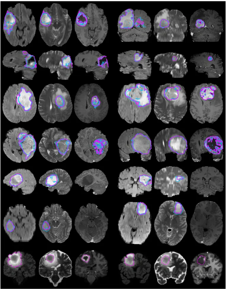
Fig. 2. Examples from the BRATS training data, with tumor regions as inferred from the annotations of individual experts (blue lines) and consensus segmentation (magenta lines). Each row shows two cases of high-grade tumor (rows 1-4), low-grade tumor (rows 5-6), or synthetic cases (last row). Images vary between axial, sagittal, and transversal views, showing for each case: FLAIR with outlines of the whole tumor region (left) ; T2 with outlines of the coreregion (center); T1c with outlines of the active tumor region if present (right). Best viewed when zooming into the electronic version of the manuscript.
TABLE II
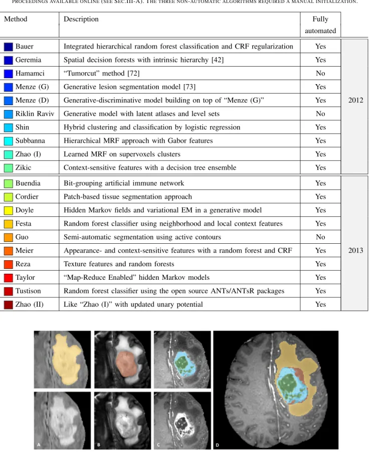
OVERVIEW OF THE ALGORITHMS EMPLOYED IN2012AND2013. FOR A FULL DESCRIPTION PLEASE REFER TO THEAPPENDIX AND THE WORKSHOP PROCEEDINGS AVAILABLE ONLINE(SEESEC.III-A). THE THREE NON-AUTOMATIC ALGORITHMS REQUIRED A MANUAL INITIALIZATION.
Method Description Fully
automated
Bauer Integrated hierarchical random forest classification and CRF regularization Yes
Geremia Spatial decision forests with intrinsic hierarchy [42] Yes
Hamamci “Tumorcut” method [72] No
Menze (G) Generative lesion segmentation model [73] Yes
Menze (D) Generative-discriminative model building on top of “Menze (G)” Yes 2012
Riklin Raviv Generative model with latent atlases and level sets No
Shin Hybrid clustering and classification by logistic regression Yes
Subbanna Hierarchical MRF approach with Gabor features Yes
Zhao (I) Learned MRF on supervoxels clusters Yes
Zikic Context-sensitive features with a decision tree ensemble Yes
Buendia Bit-grouping artificial immune network Yes
Cordier Patch-based tissue segmentation approach Yes
Doyle Hidden Markov fields and variational EM in a generative model Yes
Festa Random forest classifier using neighborhood and local context features Yes
Guo Semi-automatic segmentation using active contours No
Meier Appearance- and context-sensitive features with a random forest and CRF Yes 2013
Reza Texture features and random forests Yes
Taylor “Map-Reduce Enabled” hidden Markov models Yes
Tustison Random forest classifier using the open source ANTs/ANTsR packages Yes
Zhao (II) Like “Zhao (I)” with updated unary potential Yes
Fig. 3. Manual annotation through expert raters. Shown are image patches with the tumor structures that are annotated in the different modalities (top left) and the final labels for the whole dataset (right). The image patches show from left to right: the whole tumor visible in FLAIR (Fig. A), the tumor core visible in T2 (Fig. B), the enhancing tumor structures visible in T1c (blue), surrounding the cystic/necrotic components of the core (green) (Fig. C). The segmentations are combined to generate the final labels of the tumor structures (Fig. D): edema (yellow), non-enhancing solid core (red), necrotic/cystic core (green), enhancing core(blue).
3) The “enhancing core” of the tumor was subsequently segmented by thresholding T1c intensities within the resulting gross tumor core, including the Gadolinium enhancing tumor rim and excluding the necrotic center and vessels. The appropriate intensity threshold was determined visually on a case-by-case basis (Fig. 3 C). 4) The “necrotic (or fluid-filled) core” was defined as the tortuous, low intensity necrotic structures within the enhancing rim visible in T1c. The same label was also used for the very rare instances of hemorrhages in the BRATS data (Fig. 3 C).
5) Finally, the “non-enhancing (solid) core” structures were defined as the remaining part of the gross tumor core, i.e., after subtraction of the “enhancing core” and the “necrotic (or fluid-filled) core” structures (Fig. 3 D). Following this protocol, the MRI scans were annotated by a trained team of radiologists and altogether seven radiographers in Bern, Debrecen and Boston. They outlined structures in ev-ery third axial slice, interpolated the segmentation using mor-phological operators (region growing), and visually inspected the results in order to perform further manual corrections, if necessary. All segmentations were performed using the 3D slicer software5, taking about 60 minutes per subject. As men-tioned previously, the tumor labels used initially in the BRATS 2012 challenge contained only two classes for both high- and low-grade glioma cases: “edema”, which was defined similarly as the edema class above, and “core” representing the three core classes. The simulated data used in the 2012 challenge also had ground truth labels only for “edema” and “core”. Consensus labels: In order to deal with ambiguities in individ-ual tumor structure definitions, especially in infiltrative tumors for which clear boundaries are hard to define, we had all subjects annotated by several experts, and subsequently fused the results to obtain a single consensus segmentation for each subject. The 30 training cases were labeled by four different raters, and the test set from 2012 was annotated by three. The additional testing cases from 2013 were annotated by one rater. For the data sets with multiple annotations we fused the resulting label maps by assuming increasing “severity” of the disease from edema to non-enhancing (solid) core to necrotic (or fluid-filled) core to enhancing core, using a hierarchical majority voting scheme that assigns a voxel to the highest class to which at least half of the raters agree on (Algorithm 1). To illustrate this rule: a voxel that has been labeled as edema, edema, non-enhancing core, and necrotic core by the four annotators would be assigned to non-enhancing core structure as this is the most serious label that 50% of the experts agree on.
We chose this hierarchical majority vote to include prior knowledge about the structure and the ranking of the labels. A direct application of other multi-class fusion schemes that do not consider relations between the class labels, such as the STAPLE algorithm [69], lead to implausible fusion results where, for example, edema and normal voxels formed regions that were surrounded by “core” structures.
5www.slicer.org
Algorithm 1 The hierarchical majority vote. The number of raters/algorithms that assigned a given voxel to one of the four tumor structures is indicated by nedm, nnen, nnec, nenh; nall is the total number of raters/algorithms.
label ← “nrm” . normal tissue
if (nedm+ nnen+ nnec+ nenh) ≥ nall/2 then
label ← “edm” . edema
if (nnen+ nnec+ nenh) ≥ nall/2 then
label ← “nen” . non-enhancing core
if (nnec+ nenh) ≥ nall/2 then
label ← “nec” . necrotic core
if nenh≥ nall/2 then
label ← “enh” . enhancing core
end if end if end if end if
E. Evaluation metrics and ranking
Tumor regions used for validation.: The tumor structures rep-resent the visual information of the images, and we provided the participants with the corresponding multi-class labels to train their algorithms. For evaluating the performance of the segmentation algorithms, however, we grouped the different structures into three mutually inclusive tumor regions that better represent the clinical application tasks, for example, in tumor volumetry. We obtain
1) the “whole” tumor region (including all four tumor structures),
2) the tumor “core” region (including all tumor structures except “edema”),
3) and the “active” tumor region (only containing the “enhancing core” structures that are unique to high-grade cases).
Examples of all three regions are shown in Fig. 2. By eval-uating multiple binary segmentation tasks, we also avoid the problem of specifying misclassification costs for trading false assignments in between, for example, edema and necrotic core structures or enhancing core and normal tissue, which cannot easily be solved in a global manner.
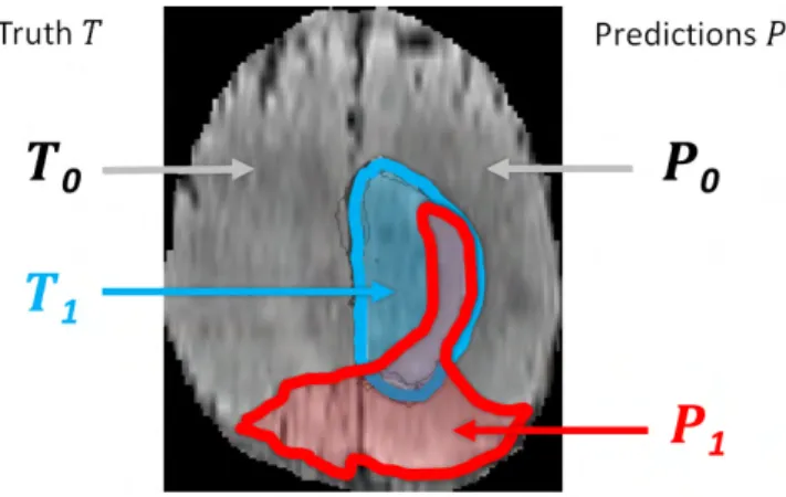
Performance scores: For each of the three tumor regions we obtained a binary map with algorithmic predictions P ∈ {0, 1} and the experts’ consensus truth T ∈ {0, 1}, and we calculated the well-known Dice score:
Dice(P, T ) = |P1∧ T1| (|P1| + |T1|)/2
,
where ∧ is the logical AND operator, | · | is the size of the set (i.e., the number of voxels belonging to it), and P1 and T1 represent the set of voxels where P = 1 and T = 1, respectively (Fig. 4). The Dice score normalizes the number
Fig. 4. Regions used for calculating Dice score, sensitivity, specificity, and robust Hausdorff score. Region T1 is the true lesion area (outline blue), T0
is the remaining normal area. P1 is the area that is predicted to be lesion
by – for example – an algorithm (outlined red), and P0 is predicted to be
normal. P1 has some overlap with T1 in the right lateral part of the lesion,
corresponding to the area referred to as P1∧ T1in the definition of the Dice
score (Eq. III-E) .
of true positives to the average size of the two segmented areas. It is identical to the F score (the harmonic mean of the precision recall curve) and can be transformed monotonously to the Jaccard score.
We also calculated the so-called sensitivity (true positive rate) and specificity (true negative rate):
Sens(P, T ) = |P1∧ T1| |T1|
and Spec(P, T ) = |P0∧ T0| |T0|
, where P0 and T0 represent voxels where P = 0 and T = 0, respectively.
Dice score, sensitivity, and specificity are measures of voxel-wise overlap of the segmented regions. A different class of scores evaluates the distance between segmentation bound-aries, i.e., the surface distance. A prominent example is the Hausdorff distance calculating for all points p on the surface ∂P1 of a given volume P1 the shortest least-squares distance d(p, t) to points t on the surface ∂T1of the other given volume T1, and vice versa, finally returning the maximum value over all d:
Haus(P, T ) = max{ sup p∈∂P1 inf t∈∂T1 d(p, t), sup t∈∂T1 inf p∈∂P1 d(t, p) } Returning the maximum over all surface distances, however, makes the Hausdorff measure very susceptible to small out-lying subregions in either P1 or T1. In our evaluation of the “active tumor” region, for example, both P1 or T1 may consist of multiple small areas or non-convex structures with high surface-to-area ratio. In the evaluation of the “whole tumor”, predictions with few false positive regions – that do not substantially affect the overall quality of the segmentation as they could be removed with an appropriate postprocessing – might also have a drastic impact on the overall Hausdorff score. To this end we used a robust version of the Hausdorff measure – reporting not the maximal surface distance between P1 and T1, but the 95% quantile of it.
Significance tests: In order to compare the performance of different methods across a set of images, we performed two types of significance tests on the distribution of their Dice scores. For the first test we identified the algorithm that performed best in terms of average Dice score for a given task, i.e., for the whole tumor region, tumor core region, or active tumor region. We then compared the distribution of the Dice scores of this “best” algorithm with the corresponding distributions of all other algorithms. In particular, we used a non-parametric Cox-Wilcoxon test, testing for significant differences at a 5% significance level, and recorded which of the alternative methods could not be distinguished from the “best” method this way.
In the same way we also compared the distribution of the inter-rater Dice scores, obtained by pooling the Dice scores across each pair of human raters and across subjects – with each subject contributing 6 scores if there are 4 raters, and 3 scores if there are 3 raters – to the distribution of the Dice scores calculated for each algorithm in a comparison with the consensus segmentation. We then recorded whenever the distribution of an algorithm could not be distinguished from the inter-rater distribution this way. We note that our inter-rater score somewhat overestimates variability as it is calculated from two manual annotations that may both be very eccentric. In the same way a comparison between a rater and the consensus label may somewhat underestimates variability, as the same manual annotations had contributed to the consensus label it now is compared against.
F. Online evaluation platforms
A central element of the BRATS benchmark is its online evaluation tool. We used two different platforms: the Vir-tual Skeleton Database (VSD), hosted at the University of Bern, and the Multimedia Digital Archiving System (MIDAS), hosted at Kitware [80]. On both systems participants can download annotated training and “blinded” test data, and upload their segmentations for the test cases. Each system automatically evaluates the performance of the uploaded label maps, and makes detailed – case by case – results available to the participant. Average scores for the different subgroups are also reported online, as well as a ranked comparison with previous results submitted for the same test sets.
The VSD6 provides an online repository system tailored to the needs of the medical research community. In addition to storing and exchanging medical image datasets, the VSD provides generic tools to process the most common image format types, includes a statistical shape modeling framework and an ontology-based searching capability. The hosted data is accessible to the community and collaborative research efforts. In addition, the VSD can be used to evaluate the submissions of competitors during and after a segmentation challenge. The BRATS data is publicly available at the VSD, allowing any team around the world to develop and test novel brain tumor segmentation algorithms. Ground truth segmentation files for the BRATS test data are hosted on the VSD but their download is protected through appropriate file permissions.
The users upload their segmentation results through a web-interface, review the uploaded segmentation and then choose to start an automatic evaluation process. The VSD automatically identifies the ground truth corresponding to the uploaded segmentations. The evaluation of the different label overlap measures used to evaluate the quality of the segmentation (such as Dice scores) runs in the background and takes less than one minute per segmentation. Individual and overall results of the evaluation are automatically published on the VSD webpage and can be downloaded as a CSV file for further statistical analysis. Currently, the VSD has evaluated more than 10 000 segmentations and recorded over 100 registered BRATS users. We used it to host both the training and test data, and to perform the evaluations of the on-site challenges. Up-to-date ranking is available at the VSD for researchers to continuously monitor new developments and streamline improvements.
MIDAS7 is an open source toolkit that is designed to manage grand challenges. The toolkit contains a collection of server, client, and stand-alone tools for data archiving, analysis, and access. This system was used in parallel with VSD for hosting the BRATS training and test data in 2012, as well as managing submissions from participants and providing final scores using a collection of metrics. It has not been used any more for the 2013 BRATS challenge.
The software that generates the comparison metrics between ground truth and user submissions in both VSD and MIDAS is available as the open source COVALIC (Comparison and Validation of Image Computing) toolkit8.
IV. RESULTS
In a first step we evaluate the variability between the segmentations of our experts in order to quantify the difficulty of the different segmentation tasks. Results of this evaluation also serve as a baseline we can use to compare our algorithms against in a second step. As combining several segmentations may potentially lead to consensus labels that are of higher quality than the individual segmentations, we perform an experiment that applies the hierarchical fusion algorithm to the automatic segmentations as a final step.
A. Inter-rater variability of manual segmentations
Fig. 5 analyzes the inter-rater variability in the four-label manual segmentations of the training scans (30 cases, 4 differ-ent raters), as well as of the final off-site test scans (15 cases, 3 raters). The results for the training and test datasets are overall very similar, although the inter-rater variability is a bit higher (lower Dice scores) in the test set, indicating that images in our training dataset were slightly easier to segment (Fig. 5, plots at the top). The scores obtained by comparing individual raters against the consensus segmentation provides an estimate of an upper limit for the performance of any algorithmic segmentation, indicating that segmenting the whole tumor region for both low- and high-grade and the tumor core region
7www.midasplatform.org
8github.com/InsightSoftwareConsortium/covalic
for high-grade is comparatively easy, while identifying the “core” in low-grade glioma and delineating the enhancing structures for high-grade cases is considerably more difficult (Fig. 5, table at the bottom). The comparison between an individual rater and the consensus segmentation, however, may be somewhat overly optimistic with respect to the upper limit of accuracy that can be obtained on the given datasets, as the consensus label is generated using the rater’s segmentation it is compared against. So we use the inter-rater variation as an unbiased proxy that we compare with the algorithmic segmentations in the remainder. This sets the bar that has to be passed by an algorithm to Dice scores in the high 80% for the whole tumor region (median 87%), to scores in the high 80% for “core” region (median 94% for high-grade, median 82% for low-grade), and to average scores in the high 70% for “active” tumor region (median 77%) (Fig. 5, table at the bottom).
We note that on all datasets and in all three segmentation tasks the dispersion of the Dice score distributions is quite high, with standard deviations of 10% and more in particular for the most difficult tasks (tumor core in low-grade patients, activecore in high-grade patients), underlining the relevance of comparing the distributions rather than comparing summary statistics such as the mean or the median and, for example, ranking measures thereof.
B. Performance of individual algorithms
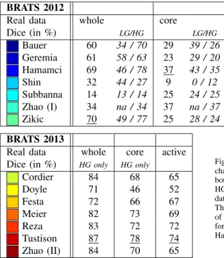
On-site evaluation: Results from the on-site evaluations are reported in Fig. 6. Synthetic images were only evaluated in the 2012 challenge, and the winning algorithms on these images were developed by Bauer, Zikic, and Hamamci (Fig. 6, top right). The same methods also ranked top on the real data in the same year (Fig. 6, top left), performing particularly well for whole tumor and core segmentation. Here, Hamamci required some user interaction for an optimal initialization, while the methods by Bauer and Zikic were fully automatic. In the 2013 on-site challenge, the winning algorithms were those by Tustison, Meier, and Reza, with Tustison performing best in all three segmentation tasks (Fig. 6, bottom left).
Overall, the performance scores from the on-site test in 2013 were higher than those in the previous off-site leaderboard evaluation (compare Fig. 7, top with Fig. 6, bottom left). As the off-site test data contained the test cases from the previous year, one may argue that the images chosen for the 2013 site evaluation were somewhat easier to segment than the on-site test images in the previous – and one should be cautious about a direct comparison of on-site results from the two challenges.
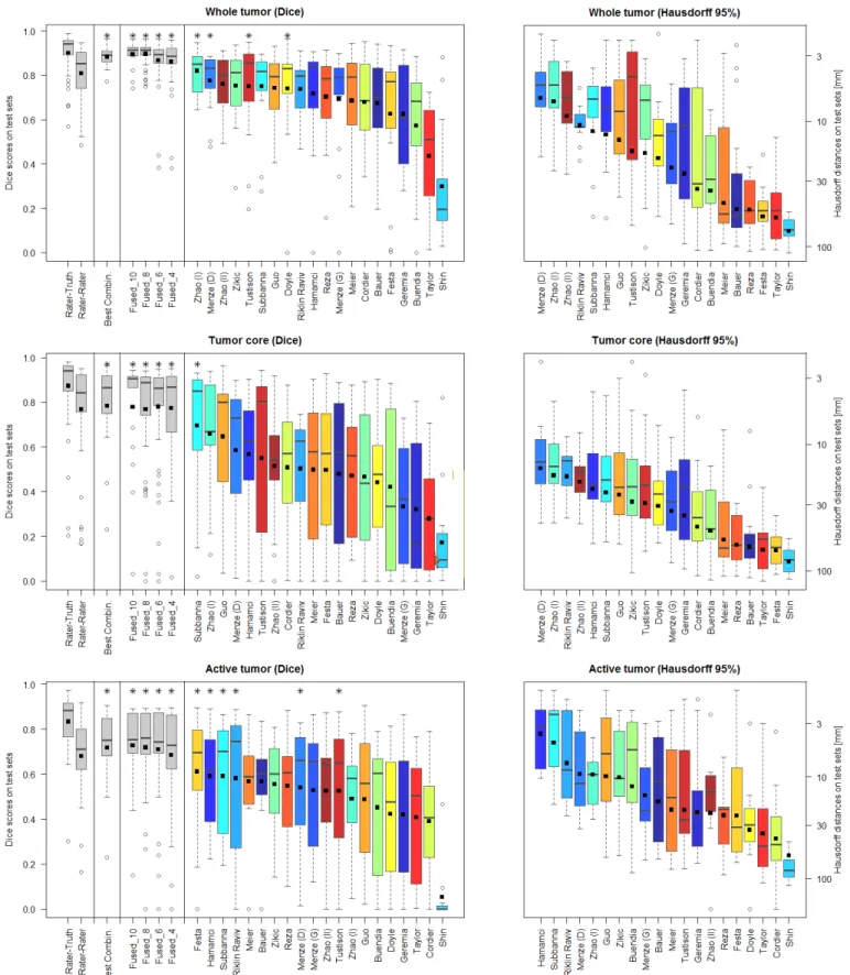
Off-site evaluation: Results on the off-site evaluation (Fig. 7 and Fig. 8) allow us to compare algorithms from both chal-lenges, and also to consider results from algorithms that did not converge within the given time limit of the on-site evalua-tion (e.g., Menze, Geremia, Riklin Raviv). We performed sig-nificance tests on the Dice score to identify which algorithms performed best or similar to the best one for each segmentation task (Fig. 7). We also performed significance tests on the
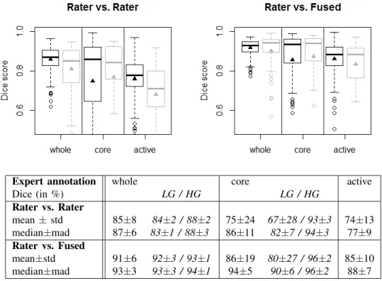
Expert annotation whole core active Dice (in %) LG / HG LG / HG Rater vs. Rater mean ± std 85±8 84±2 / 88±2 75±24 67±28 / 93±3 74±13 median±mad 87±6 83±1 / 88±3 86±11 82±7 / 94±3 77±9 Rater vs. Fused mean±std 91±6 92±3 / 93±1 86±19 80±27 / 96±2 85±10 median±mad 93±3 93±3 / 94±1 94±5 90±6 / 96±2 88±7
Fig. 5. Dice scores of inter-rater variation (top left), and variation around the “fused” consensus label (top right). Shown are results for the “whole” tumor region (including all four tumor structures), the tumor “core” region (including enhancing, non-enhancing core, and necrotic structures), and the “active” tumor region (that features the T1c enhancing structures). Black boxplots show training data (30 cases); gray boxes show results for the test data (15 cases). Scores for “active” tumor region are calculated for high-grade cases only (15/11 cases). Boxes report quartiles including the median; whiskers and dots indicate outliers (some of which are below 0.5 Dice); and triangles report mean values. The table at the bottom shows quantitative values for the training and test datasets, including scores for low- and high-grade cases (LG/HG) separately; here “std” denotes standard deviation, and “mad” denotes median absolute deviance.
Dice scores to identify which algorithms had a performance that is similar to the inter-rater variation that are indicated by stars on top of the box plots in Figure 8. For “whole” tumor segmentation, Zhao (I) was the best method, followed by Menze (D), which performed the best on low-grade cases; Zhao (I), Menze (D), Tustison, and Doyle report results with Dice scores that were similar to the inter-rater variation. For tu-mor “core” segmentation, Subbanna performed best, followed by Zhao (I) that was best on low-grade cases; only Subbanna has Dice scores similar to the inter-rater scores. For “active” core segmentation Festa performs best; with the spread of the Dice scores being rather high for the “active” tumor segmentation task, we find a high number of algorithms (Festa, Hamamci, Subbanna, Riklin Raviv, Menze (D), Tustison) to have Dice scores that do not differ significantly from those recorded for the inter-rater variation. Sensitivity and specificity varied considerably between methods (Fig. 7, bottom).
Using the Hausdorff distance metric we observe a ranking that is overall very similar (Fig. 7, boxes on the right), suggesting that the Dice scores indicate the general algorithmic performances sufficiently well. Inspecting segmentations of the one method that is an exception to this rule (Festa), we find it to segment the active region of the tumor very well for most volumes, but also to miss all voxels in the active region of three volumes (apparently removed from a very strong spatial regularization), with low Dice scores and Hausdorff distances of more than 50mm. Averaged over all patients, this still leads
to a very good Dice score, but the mean Hausdorff distance is unfavourably dominated by the three segmentations that failed. C. Performance of fused algorithms
An upper limit of algorithmic performance: One can fuse algorithmic segmentations by identifying – for each test scan and each of the three segmentation tasks – the best segmen-tation generated by any of the given algorithms. This set of “optimal” segmentations (referred to as “Best Combination” in the remainder) has an average Dice score of about 90% for the “whole” tumor region, about 80% for the tumor “core” region, and about 70% for the “active” tumor region (Fig. 7, top), surpassing the scores obtained for inter-rater variation (Fig 8). However, since fusing segmentations this way cannot be performed without actually knowing the ground truth, these values can only serve as a theoretical upper limit for the tumor segmentation algorithms being evaluated. The average Dice score of the algorithm performing best on the given task are about 10% below these numbers.
Hierarchical majority vote: In order to obtain a mechanism for fusing algorithmic segmentations in more practical settings, we first ranked the available algorithms according to their average Dice score across all cases and all three segmentation tasks, and then selected the best half. While this procedure guaranteed that we used meaningful segmentations for the subsequent pooling, we note that the resulting set included
BRATS 2012
Real data whole core
Dice (in %) LG/HG LG/HG Bauer 60 34 / 70 29 39 / 26 Geremia 61 58 / 63 23 29 / 20 Hamamci 69 46 / 78 37 43 / 35 Shin 32 44 / 27 9 0 / 12 Subbanna 14 13 / 14 25 24 / 25 Zhao (I) 34 na / 34 37 na / 37 Zikic 70 49 / 77 25 28 / 24 BRATS 2012
Synthetic data whole core
Dice (in %) LG/HG LG/HG Bauer 87 87 / 88 81 86 / 78 Geremia 83 83 / 82 62 54 / 66 Hamamci 82 74 / 85 69 46 / 80 Shin 8 4 / 10 3 2 / 4 Subbanna 81 81 / 81 41 42 / 40 Zhao (I) na na / na na na / na Zikic 91 88 / 93 86 84 / 87 BRATS 2013
Real data whole core active
Dice (in %) HG only HG only
Cordier 84 68 65 Doyle 71 46 52 Festa 72 66 67 Meier 82 73 69 Reza 83 72 72 Tustison 87 78 74 Zhao (II) 84 70 65
Fig. 6. On-site test results of the 2012 challenge (top left & right) and the 2013 challenge (bottom left), reporting average Dice scores. The test data for 2012 included both real and synthetic images, with a mix of low- and high-grade cases (LG/HG): 11/4 HG/LG cases for the real images and 10/5 HG/LG cases for the synthetic scans. All datasets from the 2012 on-site challenge featured “whole” and “core” region labels only. The on-site test set for 2013 consisted of 10 real HG cases with four-class annotations, of which “whole”, “core”, “active” regions were evaluated (see text). The best results for each task are underlined. Top performing algorithms of the on-site challenge were Hamamci, Zikic, and Bauer in 2012; and Tustison, Meier, and Reza in 2013.
algorithms that performed well in one or two tasks, but performed clearly below average in the third one. Once the 10 best algorithms were identified this way, we sampled random subsets of 4, 6, and 8 of those algorithms, and fused them using the same hierarchical majority voting scheme as for combining expert annotations (Sec. III-D). We repeated this sampling and pooling procedure ten times. The results are shown in Fig. 8 (labeled “Fused 4”, “Fused 6”, and “Fused 8”), together with the pooled results for the full set of the ten segmentations (named “Fused 10”). Exemplary segmentations for a Fused 4 sample are shown in Fig. 9 – in this case, pooling the results from Subbanna, Zhao (I), Menze (D), and Hamamci. The corresponding Dice scores are reported in the table in Fig. 7. We found that results obtained by pooling four or more algorithms always outperformed those of the best individual algorithm for the given segmentation task. The hierarchical majority voting reduces the number of segmentations with poor Dice scores, leading to very robust predictions. It pro-vides segmentations that are comparable to or better than the inter-rater Dice score, and it reaches the hypothetical limit of the “Best Combination” of case-wise algorithmic segmentations for all three tasks (Fig. 8).
V. DISCUSSION
A. Overall segmentation performance
The synthetic data was segmented very well by most algo-rithms, reaching Dice scores on the synthetic data that were much higher than those for similar real cases (Fig. 6, top left), even surpassing the inter-rater accuracies. As the synthetic datasets have a high variability in tumor shape and location, but are less variable in intensity and less artifact-loaded than the real images, these results suggest that the algorithms used are capable of dealing well with variability in shape and location of the tumor segments, provided intensities can be
calibrated in a reproducible fashion. As intensity-calibration of magnetic resonance images remains a challenging problem, a more explicit use of tumor shape information may still help to improve the performance, for example from simulated tumor shapes [81] or simulations that are adapted to the geometry of the given patients [31].
On the real data some of the automated methods reached performances similar to the inter-rater variation. The rather low scores for inter-rater variability (Dice scores in the range 74-85%) indicate that the segmentation problem was difficult even for expert human raters. In general, most algorithms were capable of segmenting the “whole” region tumor quite well, with some algorithms reaching Dice scores of 80% and more (Zhao (I) has 82%). Segmenting the tumor “core” region worked surprisingly well for high-grade gliomas, and reasonably well for low-grade cases – considering the absence of enhancements in T1c that guide segmentations for high-grade tumors – with Dice scores in the high 60% (Subbanna has 70%). Segmenting small isolated areas of the “active” region in high-grade gliomas was the most difficult task, with the top algorithms reaching Dice scores in the high 50% (Festa has 61%). Hausdorff distances of the best algorithms are around 5-10mm for the “whole” and the “active” tumor region, and about 20mm for the tumor “core” region. B. The best algorithm and caveats
This benchmark cannot answer the question of what algo-rithm is overall “best” for glioma segmentation. We found that no single algorithm among the ones tested ranked in the top 5 for all three subtasks, although Hamamci, Subbanna, Menze (D), and Zhao (I) did so for two tasks (Fig. 8; considering Dice score). The results by Guo, Menze (D), Subbanna, Tustison, and Zhao (I) were comparable in all three tasks to those of the best method for respective task (indicated in bold in Fig. 7). Menze (D), Zhao (I) and Riklin Raviv led
whole core active time (min) (arch). Dice (in %) LG/HG LG/HG Bauer 68 49/74 48 30/54 57 8 (CPU) Buendia 57 19/71 42 8/54 45 0.3 (CPU) Cordier 68 60/71 51 41/55 39 20 (Cluster) Doyle 74 63/78 44 41/45 42 15 (CPU) Festa 62 24/77 50 33/56 61 30 (CPU) Geremia 62 55/65 32 34/31 42 10 (Cluster) Guo 74 71/75 65 59/67 49 <1 (CPU) Hamamci 72 55/78 57 40/63 59 20 (CPU) Meier 69 46/77 50 36/55 57 6 (CPU) Menze (D) 78 81/76 58 58/59 54 20 (CPU) Menze (G) 69 48/77 33 9/42 53 10 (CPU) Reza 70 52/77 47 39/50 55 90 (CPU)
Riklin Raviv 74 na/74 50 na/50 58 8 (CPU)
Shin 30 28/31 17 22/15 5 8 (CPU)
Subbanna 75 55/82 70 54/75 59 70 (CPU)
Taylor 44 24/51 28 11/34 41 1 (Cluster)
Tustison 75 68/78 55 42/60 52 100 (Cluster)
Zhao (I) 82 78/84 66 60/68 49 15 (CPU)
Zhao (II) 76 67/79 51 42/55 52 20 (CPU)
Zikic 75 62/80 47 33/52 56 2 (CPU)
Best Combination 88 86 / 89 78 66 / 82 71
Fused 4 82 68 / 87 73 62 / 77 65
Fig. 7. Average Dice scores from the “off-site” test, for all algorithms submitted during BRATS 2012 & 2013. The table at the top reports average Dice scores for “whole” lesion, tumor “core” region, and “active” core region, both for the low-grade (LG) and high-grade (HG) subsets combined and considered separately. Algorithms with the best average Dice score for the given task are underlined; those indicated in bold have a Dice score distribution on the test cases that is similar to the best (see also Figure 8). “Best Combination” is the upper limit of the individual algorithmic segmentations (see text), “Fused 4” reports exemplary results when pooling results from Subbanna, Zhao (I), Menze (D), and Hamamci (see text). The reported average computation times per case are in minutes; an indication regarding CPU or Cluster based implementation is also provided. The plots at the bottom show the sensitivities and specificities of the corresponding algorithms. Colors encode the corresponding values of the different algorithms; written names have only approximate locations.
Fig. 8. Dispersion of Dice and Hausdorff scores from the “off-site” test for the individual algorithms (color coded), and various fused algorithmic segmentations (gray), shown together with the expert results taken from Fig. 5 (also shown in gray). Boxplots show quartile ranges of the scores on the test datasets; whiskers and dots indicate outliers. Black squares indicate the mean score (for Dice also shown in the table of Fig. 7), which were used here to rank the methods. Also shown are results from four ”Fused” algorithmic segmentations (see text for details), and the performance of the “Best Combination” as the upper limit of individual algorithmic performance. Methods with a star on top of the boxplot have Dice scores as high or higher than those from inter-rater variation. The Hausdorff distances are reported on a logarithmic scale.
Fig. 9. Examples from the test data set, with consensus expert annotations (yellow) and consensus of four algorithmic labels overlaid (magenta). Blue lines indicate the individual segmentations of four different algorithms (Menze (D), Subbanna, Zhao (I), Hamamci). Each row shows two cases of high-grade tumor (rows 1-5) and low-grade tumor (rows 6-7). Three images are shown for each case: FLAIR (left), T2 (center), and T1c (right). Annotated are outlines of the wholetumor (shown in FLAIR), of the core region (shown in T2), and of active tumor region (shown in T1c, if applicable). Views vary between patients with axial, sagittal and transversal intersections with the tumor center. Note that clinical low-grade cases show image changes that have been interpreted by some of the experts as enhancements in T1c.