HAL Id: hal-01228965
https://hal.archives-ouvertes.fr/hal-01228965
Submitted on 18 Oct 2017
HAL is a multi-disciplinary open access
archive for the deposit and dissemination of
sci-entific research documents, whether they are
pub-lished or not. The documents may come from
teaching and research institutions in France or
abroad, or from public or private research centers.
L’archive ouverte pluridisciplinaire HAL, est
destinée au dépôt et à la diffusion de documents
scientifiques de niveau recherche, publiés ou non,
émanant des établissements d’enseignement et de
recherche français ou étrangers, des laboratoires
publics ou privés.
Noise and offset in the IIR filtering of event-based
sampled data
Brigitte Bidégaray-Fesquet
To cite this version:
Brigitte Bidégaray-Fesquet. Noise and offset in the IIR filtering of event-based sampled data. 1st
International Conference on Event-Based Control, Communication, and Signal Processing (EBCCSP
2015) , Jun 2015, Cracovie, Poland. �10.1109/EBCCSP.2015.7300694�. �hal-01228965�
Noise and offset in the IIR filtering
of event-based sampled data
Brigitte Bidegaray-Fesquet
Grenoble Alpes University and CNRS Laboratoire Jean Kuntzmann, B.P. 53, 38041 Grenoble Cedex 9, France
Email: [email protected]
Abstract—We investigate the impact of additive noise and uncertainty on levels (offset) on the filtering of level-crossing sampled data. We therefore suppose that either the signal of the levels are affected by an error following a normal distribution with zero mean. The errors are then analyzed in terms of the standard deviation of the normal distribution. For the illustrations an IIR filter, namely Butterworth, is used, but the results have a wider range of applications.
I. INTRODUCTION
For sporadic signals which are often encountered in mobile applications, a way to reduce the power consumption is to use event-driven sampling. The obtained data are then non-uniform [1] and signal processing techniques have to be redefined. Analog-to-Digital Converters (ADCs) using a non regular samples can lead to interesting power savings compared to Nyquist ADCs [2], [3]. The sample number reduction that can be expected for signals with prescribed H¨older regularity has been investigated in [4] using a wavelet description of data.
Previous works have given equivalents of Finite Impulse Response (FIR) filters [5], [6] or Infinite Impulse Response (IIR) filters [7]. The effect of noise and offset has been of course intensively studied for classical regular signals. Here we propose a first analysis of the impact of these effects with filters specifically designed for non-uniform data.
We first describe precisely the type of data produced by the level-crossing sampling procedure and explain why we are specially interested in offset impact. Section II is devoted to the description of the implementation of filters for non-uniform data. Additive noise and offset are then addressed in Sections III and IV.
A. Level-crossing sampling
Our purpose is to write algorithms that can be used in asynchronous systems and for which the samples are obtained via an Asynchronous ADC (A-ADC) based on level-crossing sampling [8], [9]. This produces non-uniform samples in time with quantized amplitudes. Suppose we have 2M predefined levels. We use here equi-spaced levels, but the algorithms do not take this feature into account. The design of specific sets of levels for specific applications and type of signals is not addressed here.
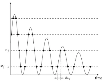
Each sample is the couple of an amplitude xj and a
time delay δtj, computed with a local clock (see Figure 1).
No global time is necessary for the implementation of the
algorithms, but, for sake of clarity, we will describe them using sample times tj. We have δtj= tj− tj−1.
time xj−1 xj • • • • • • • • • • • • • • • • • • • • • • • δtj
Fig. 1. Level-crossing sampling.
For data processing, the input analog signal only known at times tj and other information about the signal is lost.
We however need an analog signal to derive the filtering procedures and consider an (at most) linearly interpolated signal from the non-uniform samples:
x(t) ∼
n
X
j=1
(aj+ bjt)χ[tj−1,tj], (1)
where χI is the characteristic function of interval I.
B. Jitter vs. offset
There is clearly an amplitude–time duality between classi-cal regular sampling and level-crossing sampling. In classiclassi-cal sampling, samples are supposed to be taken at regular time intervals. Times are supposed to be perfectly known and multiples of some basis sampling time ts. Amplitudes are
captured at these times and have the precision of the ADC. On the contrary, in the level-crossing paradigm, levels and hence amplitudes are perfectly known, and times (or more precisely delays) are captured when a level is crossed with the precision of the local clock.
Classical jitter consists in having an incertitude on the capture time. The amplitude is not captured at the right time,
but data processing uses the theoretical regular structure, and computes as if amplitude xk is captured at time kts, inducing
a bias.
The equivalent phenomenon in level-crossing sampling is therefore an incertitude, an offset, on the amplitudes, i.e. the levels. For some reason the level which is recognized by the hardware can be slightly different from its theoretical design value. The time at which this level is crossed is slightly different from the time at which the theoretical level is crossed but the data processing is done with the theoretical amplitude. This induces a dual bias to that for classical jitter.
Except for may be one sample at the beginning or the end of the data, classical jitter does not induce a change in the number of samples. In level-crossing, an error on the level can induce changes in the number of samples if the value of the level is close to local extrema of the data (see Figure 2).
two samples no sample • •
Fig. 2. Variation of the number of samples.
In the situation shown in Figure 2 wrong values of levels can induce in particular in peak clipping.
II. NON-UNIFORMIIRFILTERS
In this paper, we will use Infinite Impulse Response (IIR) filters. The only reason is that we have to able to compare in the offset case two filtered signals at different input times, and that we have already proposed an algorithm that allows to compte the filtering result at any time, independently of the input samples times. In the non-uniform context, the z-transform formulation has no meaning. Two context have been studied and will be used here: the state representation of IIR filters [7] or the formulation in the frequency domain [10], [11].
A. Uniform filters for non-uniform data
The state representation consists in considering the usual filter coefficients αk and βk that occur in the Laplace
expres-sion of the filter transfer function ˆ h(p) = N X k=0 αkpk/ N X k=0 βkpk. (2)
Here N is the filter order. Then the filtering process consists in computing the state vector S(t), solution to the N-th order linear system dS(t) dt = AS(t) + Bx(t), (3) where A = 0 1 · · · 0 0 .. . ... . .. ... ... 0 0 · · · 1 0 0 0 · · · 0 1 −β0 −β1 · · · −βK−2 −βK−1
is the N ×N state matrix, and B = (0 · · · 0 1)tis the command
vector, and then the filtered signal y(t) is simply computed as y(t) = CS(t) + Dx(t), (4) where C = (α0 − αNβ0 · · · αN −1 − αNβN −1) is the
observation vector and D = αN the direct link coefficient.
Numerical algorithms follow from then the discretization of the differential equation (3) or its integral form
S(t) = eAtS(0) + Z t
t0
eA(t−τ )Bx(τ ) dτ (5) (see [7] for more details). The non-uniformity of data is handled by the fact that the discretization uses irregular time-steps stemming from the input data times.
B. Non-uniform filters in the frequency domain
We have also developed filters which are based on the interpolation in the frequency domain of the analog filter transfer function H. The filtered signal is then the convolution of the input signal x(t)
y(t) = Z +∞
−∞
h(t − τ )x(τ ) dτ (6) with the inverse Fourier transform of H:
h(t) = 1 2π
Z +∞
−∞
H(ω)eiωtdω. (7) Then aim of this approach is that it is possible to describe with very few filter samples equivalents of very high order filters, and even the ideal low-pass filter H(ω) = χ[−ωc,ωc] [10].
Here we sample in the frequency domain existing filter. The sampling can be done non-uniformly, i.e. with non equi-spaced frequencies. In practice we define the filter for positive values of the frequency and suppose it is symmetric. Level-crossing sampling is used to define the sampling frequencies and we obtain filter samples (ωk, Hk). We describe here linear
interpolation, but log-scale interpolation has also been studied [11]. The filter amplitudes Hk are complex and it has been
showed in [12] that the best way to perform the interpolation is to treat the absolute values and the phase of the amplitudes separately. This leads to less attenuation in the desired pass domain. For a low-pass filter linear interpolation yields a continuous approximation of H(ω): H(ω) ∼ K X k=1 n (ρ0k+ ρ 1 kω)e i(θ0 k+θ 1 kω)χJ k + (ρ0k− ρ1 kω) − e i(θ0 k−θ1kω)χ Jk− o . (8) Here Jk = [ωk−1, ωk] (ω0 = 0), J−k = [−ωk, −ωk−1], and ρ0
k, ρ1k, θk0, and θk1are computed in a straightforward way from
the filter samples (ωk, Hk).
Inserting (1) and (7) in (6) the filtered signal can be cast as y(t) = n X j=0 xj K X k=1 hjk(t), (9)
which more or less looks like a FIR filter formula, although we will interpolate IIR filter transfer functions. Details can be
found in [12] and [10]. One advantage of this approach its that we will be able to evaluated y at any time t, possibly different from times tj.
III. ADDITIVE NOISE
The goal is to compare at each data time (not changed here by the addition of noise) filtered signal y(t) obtained from the discretization of x(t) and the filtered signal ˜y(t) associated to ˜
x(t) = x(t) + ε(t) via the computation of the mean square error, weighted bu the length of each sample:
E = 1 T
X
j
(y(tj) − ˜y(tj))2δtj, (10)
where T is the total time duration of the signal.
An additive noise ε(t) is added, with zero mean and a standard deviation σ. The ε(tj) are independent identically
distributed. It is therefore expected that the mean square error will be of the order of σ2.
The SPASS MATLAB toolbox is used for numerical tests [13]. It implements a series of routines specific for the numeri-cal processing of non-uniform data. In particular it implements the A-ADC and filters described above.
For the numerical tests we use
x(t) = .5 + .25 cos(2πt) + .25 cos(4 · 2πt) (11) as input signal. The regular samples are taken at a 1000 Hz rate. The level-crossing sampling of x(t) is performed defining 2M (M = 3 or 4) equi-spaced levels ranging from .05 to .95.
There are 10.000 regular samples, 320 non-uniform samples for M = 3 and 640 non-uniform samples for M = 4.
Filtering is performed with a 5th order low-pass Butter-worth filter, with cut-off frequency 3 ·2π. The resulting filtered signal y(t) is very similar for the classical Butterworth filter and for both implementations of non-uniform filtering, state representation and frequency-domain interpolation.
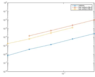
The standard deviation σ of the additive noise ε(t) is chosen to be comparable with the level quantum q. More precisely we test σ = q/4, q/2, q, and 2q. Note that q depends on M . The filtered signal ˜y is computed for the regular filter, and via state representation for M = 3 and 4. The mean square error is displayed in Figure 3 in log-log scale. The experiment is performed 10 times and a mean error is computed.
The linear behavior in log-log scale is well demonstrated by the test case. The slope of all the curves is close to 2, confirming that the mean square error is proportional to σ2. The proportion constant is dependent on the sampling and is of course much lower for the regular case which is less affected by interpolation errors in the computation of the mean square error.
IV. OFFSET
We suppose that there is an offset that is uniform over time, which means that for each realization of the normal distribution used, the set of levels is replaced by a perturbed one. This behavior can be explained for example by an experimental setting where the comparators of the A-ADC have slightly different properties as prescribed by the design.
Fig. 3. Error in presence of an additive noise; asterisk: regular case, diamond: M = 3, square M = 4.
As for the additive noise case we are interested in the mean square error between the filtered signal with an without offset. More realizations of the normal distribution will be necessary to obtain convergence, since only 2M random numbers are computed for each realization. Another feature is that the number of non-uniform samples vary from one realization to another. We therefore have to compare the signals at the same times, and use the frequency-domain algorithm for this purpose. Beside we can study the dispersion of the number of samples and compute the variance of this number.
We use the same input signal as in Section III, with M = 3 and σ = q/16, q/8, q/4, q/2, and q. The results are displayed in Figure 4. Here no comparison with the regular case is possible.
Fig. 4. Error in presence of offset.
As expected, if the offset standard deviation is of the order of the quantum, the signal and hence its filtering is too much perturbed. For smaller values of the behavior is almost linear in log-log scale (more realization should be used to have better results) and the slope is 1.8, close to 2.
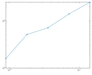
Now the variance of the number of samples is computed and displayed in Figure 5. Here again a higher number of realizations should be done to have better results, but the slope is 1. The variance of the number of samples behaves proportionally to the standard deviation.
Fig. 5. Variance of the number of samples in presence of offset.
V. CONCLUSION
We have investigated the impact of additive noise and uncertainty on levels (offset) on the IRR filtering of level-crossing sampled data. The number of levels that we use is very low and is quite sufficient to obtain filtered signals which are precise enough for the targeted applications. Besides the test cases used here are practical for filter testing since it is easy to check whether the higher frequency (4 in our case) has been filtered out or not. Of course level-crossing sampling is especially efficient in the case of sporadic signal (typically not sum of sine functions!) because of the very low number of non-linear samples compared to Nyqvist sampling. In both cases additive noise and offset, we have been able to connect the standard deviation of the applied noise (on the signal or the levels) to the mean square error between the perturbed and non perturbed signals.
Further results have to be obtained in the case when both the signal and the levels are affected by noise.
ACKNOWLEDGMENT
This work has been partially supported by the LabEx PERSYVAL-Lab (ANR-11-LABX-0025-01).
REFERENCES
[1] F. A. Marvasti, Nonuniform Sampling. Theory and Practice, ser. Information Technology: Transmission, Processing and Storage. Springer, 2001.
[2] J. W. Mark and T. D. Todd, “A nonuniform sampling approach to data compression,” IEEE Transactions on Communications, vol. 29, no. 1, pp. 24–32, January 1981.
[3] N. Sayiner, H. V. Sorensen, and T. R. Viswanathan, “A level-crossing sampling scheme for A/D conversion,” IEEE Transactions on Circuits and Systems II, vol. 43, no. 4, pp. 335–339, April 1996.
[4] B. Bid´egaray-Fesquet and M. Clausel, “Data driven sampling of oscillating signals,” Sampling Theory in Signal and Image Processing, vol. 13, no. 2, pp. 175–187, 2014.
[5] F. Aeschlimann, E. Allier, L. Fesquet, and M. Renaudin, “Asynchronous FIR filters: Towards a new digital processing chain,” in 10th International Symposium on Asynchronous Circuits and Systems (Async’04). Hersonisos, Crete: IEEE, April 2004, pp. 198–206. [6] S. M. Qaisar, L. Fesquet, and M. Renaudin, “Adaptive rate filtering
for a signal driven sampling scheme,” in International Conference on Acoustics, Speech, and Signal Processing, ICASSP 2007, vol. 3, Honolulu, Hawai‘i, USA, April 2007, pp. 1465–1568.
[7] L. Fesquet and B. Bid´egaray-Fesquet, “IIR digital filtering of non-uniformly sampled signals via state representation,” Signal Processing, vol. 90, no. 10, pp. 2811–2821, October 2010.
[8] F. Akopyan, R. Manohar, and A. B. Apsel, “A level-crossing flash asynchronous analog-to-digital converter,” in 12th IEEE International Symposium on Asynchronous Circuits and Systems (ASYNC’06), Grenoble, France, March 2006, pp. 11–22.
[9] E. Allier, G. Sicard, L. Fesquet, and M. Renaudin, “A new class of asynchronous A/D converters based on time quantization,” in 9th International Symposium on Asynchronous Circuits and Systems, Async’03. Vancouver, Canada: IEEE, May 2003, pp. 196–205. [10] B. Bid´egaray-Fesquet and L. Fesquet, “A fully non-uniform approach
to FIR filtering,” in 8th International Conference on Sampling Theory and Applications (SampTa’09), L. Fesquet and B. Torr´esani, Eds., Marseille, France, May 2009. [Online]. Available: http://hal.archives-ouvertes.fr/hal-00453350/fr/
[11] ——, “Non-uniform filter design in the log-scale,” in 9th International Conference on Sampling Theory and Application (SampTA 2011), Singapour, 2011.
[12] ——, “Non-uniform filter interpolation in the frequency domain,” Sampling Theory in Signal and Image Processing, vol. 10, no. 1–2, pp. 17–35, 2011.
[13] ——, “SPASS 2.0: Signal Processing for ASynchronous Systems,” Software, May 2010. [Online]. Available: http://ljk.imag.fr/membres/Brigitte.Bidegaray/SPASS/