Computer-aided engineering methodology for structural optimization and control

COMPUTER-AIDED ENGINEERING METHODOLOGY FOR

STRUCTURAL OPTIMIZATION AND CONTROL

By

YI-MEI MARIA CHOW

Master of Engineering in Civil and Environmental Engineering at the

Massachusetts Institute of Technology June 1998

Submitted to the Department of Civil and Environmental Engineering In Partial Fulfillment of the Requirement for the Degree of

Civil Engineer's Degree at the

Massachusetts Institute of Technology

February 2000

Copyright 0 1999 Massachusetts Institute of Technology All Right Reserve

The author hereby grants to MIT permission to reproduce and to distribute publicly paper and electronic copies of this thesis document in whole or in part.

Signature of Author

Yi-Mei Maria Chow September 15, 1999

Certified by

Jerome J. Connor Professor, Department of Civil and Environmental Engineering Thesis Supervisor

Approved by

5ldJACHUSETTS INSTITUTE OF TFCHNOLOGY

Daniele Veneziano, Chairman, Departmental Committee on Graduate Studies.

COMPUTER-AIDED ENGINEERING METHODOLOGY FOR

STRUCTURAL OPTIMIZATION AND CONTROL

By

YI-MEI MARIA CHOW

Submitted to the Department of Civil and Environmental Engineering on September 15 1999

In Partial Fulfillment of the Requirement for the Degree of Civil Engineer's Degree

ABSTRACT

The evolution of computer-aided engineering methodology has played a major role in the advancement of traditional structural engineering. It has allowed engineers to obtain better solutions for design and analysis problems by means of diverse user-friendly software packages. However, as the precision and safety requirements have increased in the ever-changing world, civil and structural engineers face numberless unsolved issues with respect to structural optimization and control.

Matlab is a very useful CAE tool for numerical analysis. In this dissertation, the computational algorithms for several vibration control systems are implemented with Matlab and used for diverse simulation studies. Matlab has many embedded tools which simplify matrix operations encountered in the vibration control. Furthermore, newly developed approaches such as evolution strategy, genetic algorithm, finite element, and neural networks form the paradigm of software elaboration in structural engineering field. Those modem numerical CAE methodologies, in addition to analytical solutions, enable further structural optimization and topological modification accomplished by computer

simulation.

With the progression in programming languages and software packages, computer-aided engineering methodology has significantly advanced the practice of structural engineering. In addition to providing the ability to model the structural behavior under static or dynamic load, newly developed web-interfaced CAE tools allow for easy access and transport information which eventually benefits structural engineering work.

Thesis Supervisor: Jerome J. Connor

ACKNOWLEDGEMENTS

I would like to take this opportunity to express my gratitude to my advisor, Professor

Jerome J. Connor, for his support, guidance, and inspiration. I enjoyed and learned a lot from every meeting and discussion we had been having during the Master of Engineering Program with the specialty of High Performance Structure. I definitely admire his rich knowledge and experience, as well as his broad viewpoint towards the innovative technology in both Structural Engineering and Information Technology.

Additionally, I would like to thank Professor John Williams and Professor Kevin Amaratunga for accepting me to the Information Technology Program for my second year graduate study at MIT. I enjoyed taking courses and working on group projects in the classes they offered regarding Computer-Aided Engineering and Software Developing. This valuable experience will surely build a bridge between my master study at MIT and

future Ph.D. study at Carnegie Mellon University.

I am also grateful to all the people in my office, and friends who have been there for me

for the past two years. Karen, Justin, Yo-Ming, Yi-san, Chun-Yi and Ching-Yu, thanks for your 'technical support'. Roxy, Bruce, Eric, Kathy, Pei-ting, Ching-yin. I will always remember how we sheared our thoughts, our minds and our hearts! Special thanks for my family friend George who constantly supports me to overcome all difficulties at school.

And, finally, Daddy and Mommy, thanks for being wonderfully supportive. I will keep going and try my best.

[TABLE OF CONTENT] A B STR A C T ... 2 ACKNOWLEDGEMENTS... 3 CHAPTER I: INTRODUCTION... 7 1.1 M OTIVATION ... 7 1.2 INN O VATION ... 8 1.3 A PPLICATION ... 9

CHAPTER II: CAE METHODOLOGY ON MATLAB... 13

2.1 FROM MATHEMATICAL MODEL TO STRUCTURAL CONTROL ... 13

2.2 SPRING-M ASS-DAMPER SYSTEM ... 14

2.3 STRUCTURAL CONTROL SYSTEM PERFORMANCE ... 18

2.4 MECHANICAL VIBRATION ON STRUCTURAL DYNAMICS ... 20

CHAPTER III: STRUCTURAL OPTIMIZATION AND CONTROL USING CAE ... 27

3.1 DISCRETE STRUCTURAL OPTIMIZATION USING EVOLUTION STRATEGIES ... 27

3.1.1 The Definition and Concept of Evolution Strategies ... 27

3.1.2 Mathematical Formulation of the Evolution Strategies... 28

3.1.3 Ten-Bar Truss: An Example... 30

3.2 TOPOLOGICAL DESIGN OF TRUSS STRUCTURE... 32

3.2.1 Problem Formulation and Solution Strategy... 33

3.2.2 Structural Optimization and Topology Modification... 34

3.2.3 Generic Algorithm and FEM Applied on Aesthetic Design of Structures... 37

3.3 THE APPLICATION OF NEURAL NETWORK ON VIBRATION CONTROL OF STRUCTURES... 38

3.3.1 Introduction to the Neural Network... 39

3.3.2 The Modeling and Thinking Methodology... 40

3.3.3 M ulti-Layer Perception ... 41

3.3.4 Use of Neural Network for Structural Optimization and Control... 44

3.4 NEURAL NETWORKS AND STRUCTURAL DESIGN... 45

3.4.1 Neural Networks as Approximation... 46

3.4.2 Polynom ial Approximation... 47

3.4.3 Neural Network Approximation is Superior to Polynomial Approximation... 48

3.4.4 Parallel Training of Neural Networks for Finite Element Mesh Generation ... 49

CHAPTER IV: CASE STUDIES IN STRUCTURAL ENGINEERING USING MATLAB... 52

4.1 GROUND M OTION EXCITATION... 52

4.2 ANIMATION OF BENDING M OMENT DIAGRAM ... 56

4.3 BENDING M OMENT CAUSED BY A MOVING VEHICLE ... 59

CHAPTER V: COMPUTER-AIDED ENGINEERING TO-THE-DATE ... 62

5.1 SOFTWARE DEVELOPMENT IN CIVIL ENGINEERING INDUSTRY ... 63

5.2 IMPACT OF CAE TO STRUCTURAL DESIGN BASED ON OPTIMIZATION CONCEPT... 65

5.3 OVERALL DESIGN FINALIZATION... 66

5.4 LOADING SPECIFICATION FOR SIMULATION ... 67

5.5 SUMMARY OF CAE SOFTWARE DESIGN GUIDELINE ... 68

CHAPTER VI: CONCLUSION AND FUTURE OUTLOOK... 69

6.1 SOFTWARE DEVELOPMENT AND INFORMATION TECHNOLOGY IN CIVIL ENGINEERING... 69

6.2 BUILDING ON THE WEB-- FACING THE NEW TREND ... 70

6.3 HIGH-TECHNOLOGY REVOLUTION COMES TO STRUCTURAL ENGINEERING ... 71

[REFERENCES]... 73 [APPENDIXES]... 75 APPENDIX [1]... 75 APPENDIX [2]... 78 APPENDIX [3]... 79 APPENDIX [4]... 80 APPENDIX [5]... 82 APPENDIX [6]... 83 APPENDIX [7]... 84 APPENDIX [8]... 86 APPENDIX [9]... 87 APPENDIX [10]... 88 [LIST OF TABLES] TABLE 1 : COMPARING EXACT-ANALYTICAL AND APPROXIMATE-DISCRETIZED FORMULATION ... 8

TABLE 2: SOLUTION OF THE TEN-BAR TRUSS... 31

TABLE 3: DATA OF THE 5-STORY BUILDING ... 54

[LIST OF FIGURES]

FIGURE 1: USE OF TOPOLOGY AND SHAPE OPTIMIZATION IN THE DESIGN PROCESS... 9

FIGURE 2: FLOW CHART OF THE BUBBLE METHOD ... 10

FIGURE 3: MATLAB OUTPUT OF BRIDGE STRUCTURAL VIBRATION--12 MODES PRESENTED... 12

FIGURE 4: 1-D SPRING-MASS-DAMPER MECHANICAL SYSTEM ... 15

FIGURE 5: RESPONSE OF A SPRING-MASS-DAMPER SYSTEM ... 17

FIGURE 6: SINGLE-LOOP SECOND-ORDER FEEDBACK SYSTEM... 19

FIGURE 7: STEP RESPONSE OF THE SECOND-ORDER SYSTEM... 20

FIGURE 8: ONE DEGREE-OF-FREEDOM STRUCTURAL SYSTEM SUBJECTED TO DYNAMIC LOAD ... 21

F IG URE 9: F(1,167)=1 ... 24

FIGURE 10: F=SIN(WN*T)**********************************''*****************... 24

FIGURE 11: CRITICAL DAMPING C=2% ... 25

FIGURE 12: STEP FUNCTION STARTING AT T=0... 25

FIGURE 13: F=ZEROS(1,1000) ; No STEP FUNCTION ... 26

FIGURE 14: TEN-BAR TRUSS USING EVOLUTION STRATEGIES... 31

FIGURE 15: EXAMPLE OF A PATH TO PERFORM A MODIFICATION IN THE TOPOLOGY ... 36

FIGURE 16: MULTI-LAYER PERCEPTION (MLP) NEURAL NETWORK... 41

FIGURE 17: THE SIGMOIDAL ACTIVATION FUNCTION. ... 43

FIGURE 18: FIVE B AR T RUSS ... 48

FIGURE 19: THE INPUT AND OUTPUT OF NEURAL NETWORK ... 50

FIGURE 20: B UILDING L AYOUT ... 55

FIGURE 21: M ATLAB R ESPONSE G RAPH... 55

FIGURE 22: SIMPLY-SUPPORTED BRIDGE... 56

FIGURE 23: BENDING MOMENT DIAGRAM OF A MOVING VEHICLE ON A BRIDGE ... 57

FIGURE 24: BENDING MOMENT PRODUCED BY VEHICLE ALONG A SIMPLY-SUPPORTED BEAM ... 58

FIGURE 26: 3-D CONTOUR OF THE SIMULATION DATA ... 61

FIGURE 25: 3-D SPIRAL DATA PLOTTING ... 61

FIGURE 27: FLOW CHART OF THE CAE METHODOLOGY IN STRUCTURAL DESIGN AND ANALYSIS ... 62

FIGURE 28: (A) STAIR DRAW CONFIGURATION (B) LADDER DRAW UTILITY ... 63

FIGURE 29: AUTO-DIMENSIONING OF THE BEAM TO COLUMN CONNECTION... 64

FIGURE 30: (A) STRUCTURAL ELEMENT DIMENSIONS (B) STRUCTURAL LAYOUT ILLUSTRATION ... 65

FIGURE 31: DEFINING THE STRUCTURAL SECTION AND SHOWING THE PROPERTIES... 67

Chapter I

1.1 Motivation

In the past several decades, civil engineering in general and structural

engineering in particular have achieved remarkable success in employing computational

support technologies. Useful tools for specific process steps, notably preliminary design

and simulation, have been developed for many advanced structural optimization and

control cases under static or dynamic load [1]. However, the full integration of future

computing capabilities into structural engineering is a challenge to civil and structural

engineers who use computer technology to implement the design methodology.

Among all the topics related to civil or structural engineering, optimization on

form and function, and control of structural system appear to be two of the most

important topics in computer-aided engineering methodology. Owing to the mathematical

complexity of structural analysis and control, engineers are seeking better ways to

simplify the tedious calculations required to optimize the performance. With the advances

in computer programming languages and the concurrent development in software product

for design and analysis, structural engineers can obtain numerical results from compiling

1.2 Innovation

Several innovative methodologies are widely applied to engineering simulation. In recent years, topology has been incorporated in structural optimization. Topology is concerned the pattern of connectivity or spatial sequence of members and elements in the entire structure [2]. Optimization of the structure is usually obtained with computer simulation. Table 1 illustrated the differences between exact analytical formulation and approximate computer simulation in structural design:

Table 1: Comparing Exact-Analytical and Approximate-Discretized Formulation

Comutaieml MthAnalytical Numerical

Continuum Discretized (FEM)

Sitn P Simultaneous Solution of Interactive Solution

All Equations

t Structure Universe Ground Structure (Finite but

(Infinite No. of Members) Large Number of Members)

Zero Small

(or Zero)

By Hand By Computer

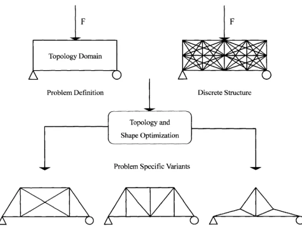
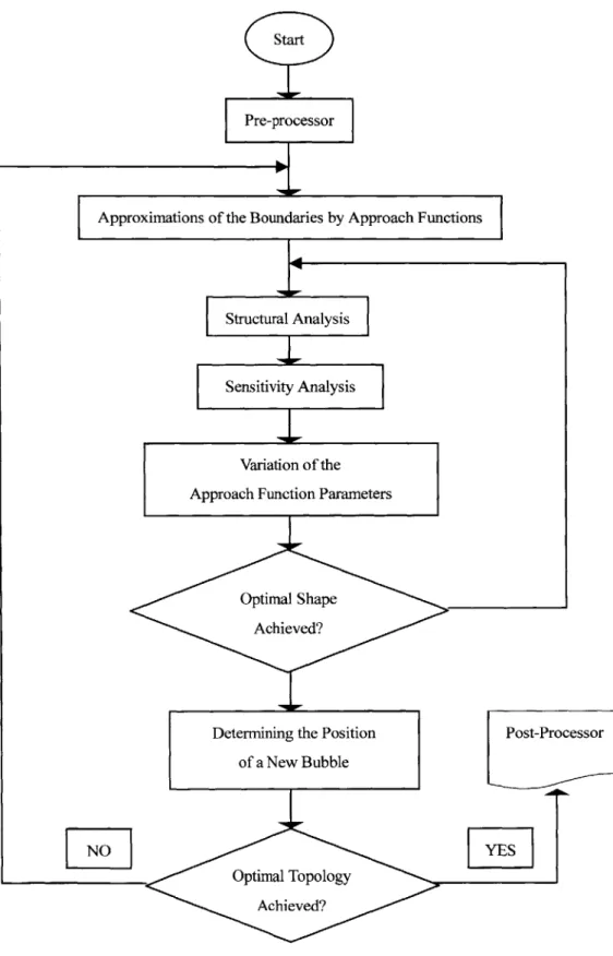
Figures 1 and 2 illustrate a particular coupling of topology and structural shape

optimization, called the "Bubble-Method' [3]. Its basic idea is the interactive positioning

of modified components into a given design domain. Resulting from the increasing

demands on the efficiency, reliability and shortened development cycle of bridge or

building structure, it has become inevitable to solve problems by computer-based

procedures. Substantial progress has been achieved in the structural computation of

F

Problem Definition Discrete Structure

Problem Specific Variants

A

C)A

CA(

Figure 1: Use of Topology and Shape Optimization in the Design Process

1.3 Application

Some programming languages are very suitable to apply on the computer-aided

engineering on structural optimization and control. For instance, Matlab has very

powerful functions for dynamic analysis and graphical representation of the output. In

Figure 3a-31, twelve modes of a bridge under vibration are illustrated with the

deformation of the truss structure. At the same time, Matlab code, which generates the

graphs, is presented in Appendix [1] at the end of this thesis.

Figure 2: Flow Chart of the Bubble Method

NO]

Fig. (3d) Fourth Mode Vibration Displacement

Fig. (3b) Second Mode Vibration Displacement.

Fig. (3c) Third Mode Vibration Displacement.

Fig. (3e) Fifth Mode Vibration Displacement

Fig. (3f) Sixth Mode Vibration Displacement Fig. (3a) First Mode Vibration Displacement

Fig. (3g) Seventh Mode Vibration Displacement

Fig. (3h) Eighth Mode Vibration Displacement

Fig. (3i) Ninth Mode Vibration Displacement

Fig. (3k) Eleventh Mode Vibration Displacement

Fig. (31) Twelfth Mode Vibration Displacement

Figure 3: Matlab Output of Bridge Structural Vibration--12 Modes Presented

Chapter II

Among civil engineering students, structural engineers and academic faculty, Matlab is becoming increasingly popular because of its features such as interactive mode

of work, immediate graphing facilities, built-in functions, the possibility of adding user-written syntax and simple programming. Also, data sets as well as options for keeping records of calculation result can be later transformed into technical reports [5]. For example, in some case studies of control theories presented in the second and the fourth

chapter of this dissertation, the numerical data and output graphics can be generated into

different window objects to be inserted and linked to another document. Besides, Matlab

operates simple coding syntax which is very similar to scientific or engineering

declarations. As a result, structural engineers will benefit from this handy tool for logic

operation of preliminary simulation.

2.1 From Mathematical Model to Structural Control

The design and analysis of structural control systems is based on mathematical

models of complex physical systems. The mathematical models, which derive from the

physical or mechanical lows of the process, are generally highly coupled with advanced engineering mathematics such as nonlinear differential equations [6]. Fortunately, with the

modem computer languages, many abstract physical or mechanical systems can be modeled to behave linearly around an operating point within some range of the variables.

The Laplace Transform method is one way to compute the solution of differential equation (7]. It is also possible to develop linear approximation to the structural or mechanical system. Furthermore, it can be used to obtain an input-output description of the linear, time-invariant (LTI) system in the form of a transfer function in structural vibration control. The application of many classical and modem control system

design and analysis tools is based on LTI mathematical models. Particularly, Matlab can be utilized with LTI systems given in the form of transfer function descriptions or

state-space description in advanced structural dynamics or seismic engineering [5].

In the following paragraphs, several case studies together with Matlab program demonstrate that Computer-Aided Engineering Methodology can be used for simulation

and visualization of the results of preliminary structural optimal control of a dynamic

system.

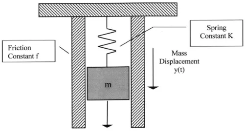
2.2 Spring-Mass-Damper System

A spring-mass-damper mechanical system is shown in Figure 4 as a simplified

structural component. The motion of the mass, denoted by y(t), is described by the

differential equation:

Friction Constant f Spring Constant K Mass Displacement y(t)

Figure 4: 1-D Spring-Mass-Damper Mechanical System

The solution, y(t), of the differential equation describes the displacement of the

mass as a function of time. The forcing function is represented by r(t). These ideal models for the spring and damper are based on lumped, linear, dynamic elements and

only approximate the actual elements.

In order to illustrate the usefulness of the Laplace transformation and the steps

involved in the system analysis, rewrite Equation (1) to:

d 2_{y dy}

M 2 ₊ f _{+ Ky = r(t) Equation (2)}

dt2 dt

We wish to obtain the response, y, as a function of time. The Laplace transform of

Equation (2) is:

M s2_{Y(s) - sy(O*) - dy(0) +}

_f(sY(s)

y(O)= Y0, Equation (3) dy ItO=0 tO =0, dit-when r(t) = 0,

we have

Ms2_Y(s)

- Msy₀ + fsY(s) -

fyo

(Ms +

f)y

Ms2 _{+fs+K (S2} +(f/M)s+K/M) S2 +2 os+ 2

Equation (4)

Equation (5)

Our objective is to design an active control system to make the structural more

stable under dynamic loading. In Equation (5), w,, =sqrt(K/M) is the natural frequency of

the system and =f/2*[sqt(KM)] is the dimensionless damping ratio. In the following

paragraphs, the control design and subsequent analysis would be based on the model

described before. We will soon see how to use Matlab to enhance our structural control

design and analysis capability.

The unforced dynamic response, y(t), of the spring-mass-damper mechanical

system is:

y(t)= e- "' sin(con 1-2t +) Equation (6)

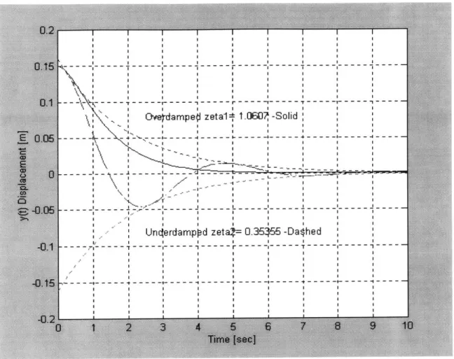
where O--cos-' . The initial displacement is y(O). The transient system response is underdamped when 4<1, overdamped when 4>1, and criticallydamped when g=l. We can

use Matlab to visualized the unforced time response of the mass displacement following

an initial displacement of y(O). Consider the overdamped and underdamped cases:

y(O)=O. 15m, y(0)=O. 1 5m, q,=sqrt2 (rad/sec), ,=3/[2sqrt(2)] 9,=sqrt2 (rad/sec), 2=1/[2sqrt(2)] [(K/M)=2, (f/M)=3] [(K/M)=2, (f/M)=3] U U Case 1: Case 2:

Figure 5: Response of a Spring-Mass-Damper System

The Matlab commands to generate the plot of unforced response are shown in Appendix [2]. In the Matlab setup, the variables y(O), On, $1 and #2 are inputs to the

workplace at the command level. Then the script <unforced.m> is executed to generate the desired plots. This creates an interactive analysis capability to analyze the effects of natural frequency and damping on the unforced response of the mass displacement.

Figure 5 shows the plotting result generated by the Matlab function. One can investigate the effect of varying the natural frequency and the damping on the time response by simply changing the values of con, #1 or (2 in the command syntax and

executing the <unforced.m> program again. Notice that the script automatically labels the

plot with the values of the damping coefficients. This avoids confusion when making many interactive simulations. The natural frequency value (zeta) could also be automatically labeled on the plot. Utilizing scripts is an important aspect of developing an effective interactive program in computer-aided design and analysis capability in Matlab. Since one can relate the natural frequency and damping to the spring constant, K, and frictionf, one can also analyze the effects of K andfon the response.

In the spring-mass-damper problem, the unforced solution to the differential

equation was readily available. In general, when simulating close-loop feedback control

systems subjected to a variety of inputs and initial conditions, it is not feasible to attempt

to obtain the solution analytically. In these cases, it is very convenient to use Matlab to

compute the solution numerically and to display the solution graphically [7]. Noted that

Matlab is one of the many useful programs of doing computer-aided engineering in

structural optimization and control. Users can always select their favorite CAE tools.

2.3 Structural Control System Performance

Primary concerns in structural control system design are stability and

performance. In order to design and analyze structural control systems, we must first

establish adequate performance specifications to be presented in the time domain or the

frequency domain. Time-domain specifications generally take the form of setting time,

percent overshoot, rise time and steady-state error specification. In this section, a Matlab

Time-domain performance specifications are generally given in terms of the transient response of a system to a given input signal, for example, seismic wave or dynamic loading histogram (8]. Since the actual input signals are usually unknown, a standard test input signal is used in the following case study and coding example can be found in Appendix [3]. The test signal is of the general form:

r(t) = t" Equation (7)

and the corresponding Laplace transform is:

R(s) = n! _n+1 Equation (8)

S

when n=2, R(s) is defined as a step function, which is shown in the block diagram in Figure 6 below:

R(s) ss___ C(s)

Figure 6: Single-Loop Second-Order Feedback System

Consider this second-order system, the close-loop output is:

co2

C s 2 +2 + ₂ R(s) _{Equation (9)}

From the above equation, one can tell that this output is similar to the step response

function, which is plotted in Figure 7. Besides, the feedback control system has the

1. decrease the sensibility of the system to plant variation

2. enable adjustment of the system transient response

3. reject disturbances and

4. reduce steady-state tracking errors

Figure 7: Step Response of the Second-Order System

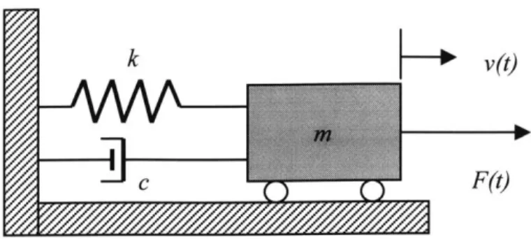
2.4 Mechanical Vibration on Structural Dynamics

In this case study, we are going to use Matlab to compute the response of a

single degree of freedom system to an arbitrary forcing function. The intent is to take

advantage of Matlab function such as convolution operation for the analysis of dynamic

k

-M--v(t)

F(t)

Figure 8: One Degree-of-freedom Structural System Subjected to Dynamic Load

For the system shown in Figure 8, the equation of motion is:

mi + c + kv = F(t) Equation (10)

The impulse response of the above system is defined as the solution of

Equation (10) when F(t)=9('t). The impulse response function h(t) is given by:

1 x sin(codt)x e-4""t h(t) Mmd 0 when t > 0 when t < 0 Equation (11)

where co,,= (k/m) is the undamped natural frequency, c,= w[sqrt(14-)] is the

damped frequency, and =c/2[sqrt(k*m)] is the damped ratio. The response of the above

system to any arbitrary forcing function F(t) can then be computed as the convolution of

this forcing function with the system's impulse response h(t):

Because of causality, the above expression becomes:

v(t) =

f

f

In the Matlab program listed in Appendix [4], one can compute the response function v(t) of a single degree of freedom system when the excitation F(t) is an arbitrary function that a structural or mechanical engineer might define.

The program prompts the user to input the M, C, and K values (with any

consistent system of units) and then calculates and displays the impulse response function.

For example, one might try M= 1 kg, C= 0.05N/ (m/s), K= 4 N/m. It also displays the

undamped natural frequency in rad/s and Hz, as well as the damping ratio Zt.

Additionally, it computes the value of 1/(M*wd), the coefficient of the impulse response

function h(t=0). For a lightly damped system this should be about the peak value of h(t).

The response to any input can be obtained by convoluting the impulse response

h(t), with that of an arbitrary excitation vector. To do this, one needs to edit this file <convol.m> and modify the excitation vector, e.g., letf=sin(z*t).

Because we want our response to die out completely over our time axis, we will

make the length of the time axis four times the time constant T, which is defined as,

T=1/(Zt*co,). This is the length of time required for the impulse response function to decrease by the factor 1le.

While executing this computer program, one has to enter numerical values for

the system's parameters. Once all three numbers (M, C, K) are entered, the impulse response h(t) and the excitation force F(t) will be plotted, and the response function v(t)

will also be showed along with the "Matlab Graph Window" [5].

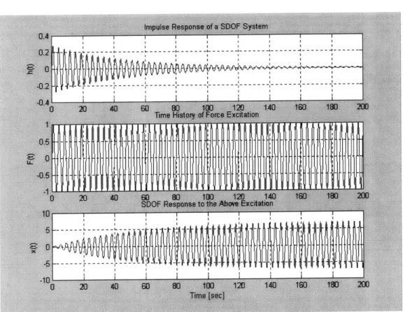
The forcing function we have used in the <convol.m> program is a delayed

impulse. By modifying the Matlab syntax and re-running the program, the corresponding

result will be displayed in Figure 9 to Figure 13. It is very convenient to compare the

three diagrams of impulse response, time history, and response to the excitation at the

same time from the Matlab plotting. In the first case, the forcing function is a single pulse

of height 1.0 and width DT=0.16 seconds. This value was delayed by 167=(500/3)

timesteps. The response x(t) is plotted in the third graphs of the output figure.

The Matlab convolution is a numerical integration. The discrete time step, DT,

in the <convol.m> program is a function of damping. However, this is only a result of

programming choice not physics [9]. In fact, DT=4*T/1000, where T=1/(Zt*Wn), and Zt is defined as the damping ration in the program. If the selected damping ratio is too small,

the number of time steps in one cycle of motion is too few and the numerical integration

is inaccurate.

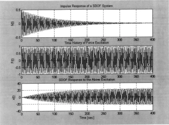
Figure 10 is the output after editing the program and substituting F(t)=sin(co,*t).

The damping value is assigned to be 2% of critical damping. Since the excitation

frequency equals the natural frequency, this is resonant excitation with a transient buildup

Figure 9: f(1,167)=1

Figure 11: Critical Damping c=2%

Figure 13: f=zeros(1,1000) ; No Step Function

By modifying the Matlab code, try two other frequencies, such as 0.4 and 3

times the natural frequency, i.e. let F(t)=sin(.4*W,*t) and F(t)=sin(3*con*t). In other

words, one can see if the stiffness controlled or mass controlled steady state response

Chapter III

AND

In this chapter, certain mathematical or mechanical CAE models for solving

special structural design problems will be presented. To develop a sophisticated CAE tool

particularly for structural optimization and control, the algorithm and methodology are

the most important parts of the prototype. Additionally, new concepts have been brought

to civil and structural engineering from computer science and operation research to

improve the performance to the ultimate structural design.

3.1 Discrete Structural Optimization Using Evolution Strategies

3.1.1 The Definition and Concept of Evolution Strategies

In recent years, several new methods to handle discrete structural optimization

have been developed. For example, the evolution strategies (ESs), which imitate

biological evolution in nature, have been converted to the computer algorithm applied to

continuous optimization problem [101. Instead of solving a single design point in the

conventional structural engineering task, the ESs work simultaneously with a group of

design points in the space of variables. The basic concept of ESs presents a method of sequential linear discrete programming and converts the nonlinear discrete problem into a

approximation to the mixed-discrete nonlinear programming problem by combining a sequential linear one with a branch and bound algorithm.

Once the continuous problem has been transformed into a discrete task to be executed iteratively by computer, the structural design can be completed with less error and time. In the following section, two examples illustrating the use of evolution strategies (two-member ESs and multi-member ESs) will be presented. With of this

procedure, a nonlinear discrete structural optimization problem can be solved.

3.1.2 Mathematical Formulation of the Evolution Strategies

In general, a structural optimization problem can be represented as a nonlinear

mathematical computer-programming problem as the following form [10]:

minimize f(X) X ( E"

subject to g.(X) > 0, i =1,2,..., m.

First of all, to solve the above equation, the two-membered evolution strategies

work in two steps:

<Step 1: Mutation>

In the gth generation a new design-vector is computed from where XO and Xp are the

offspring and parent vectors, respectively:

Z ()=[z (g), Z2 (), ... , z (g)]T is a normally distributed random vector whose components z,(9)

has a probability density function:

Az) 1 (Z -_)2

p2z, = 2exp[ Equation (16)

The design purpose of the computer program should fulfill the requirement that the expectation 5, should be zero and the variation of should be small.

<Step 2: Selection>

The selection chooses the best individual between the parent and offspring to match the conditions described:

= Xg) if g,(X))> 0, i=1,..., m and f(X(,)) f(Xfg));

P X (g otherwise,

Equation (17)

Usually, Z( has the role of mutation. The standard deviation o-can be considered as a

step length which is adjusted during the search success of the computer algorithm.

Secondly, in the case of multi-membered ESs, a population of parent vector and offspring vector will be handled simultaneously, and the operator recombination as well

as the idea of self-adaptation of strategy parameters [10] is incorporated:

<Step1: Recombination and Mutation>

In the gth generation, k offspring vectors are created by means of recombination and mutation.

<Step2: Selection>

(p+A)-ES: The best p individuals are selected out of parents and offsprings to form the parents of the next generation. This is so-called the "genetic

algorithm" for the iteration of the computer program.

(p,A)-ES: The best p individuals are selected only from the A offsprings. The m parents in the gth generation die out. This is defined as the process of

"optimization".

3.1.3 Ten-Bar Truss: An Example

The well-known 10-bar truss problem shown in Figure 14 will be analyzed by

the evolution strategy [12]. The objective functionf(X) of this problem is the weight of the structure itself. The design variables g/(Xo) are the cross-sectional areas of the 10

members. The constraints f(Xo(9) and f(Xpg) are the member stresses and the vertical

displacement of the node 2 and 4. The allowable displacement is limited to 2 inches and

the allowable stress is limited to ± 25 ksi. The design parameters are:

E= 104 ksi E states as Young's Modulus of the structure component.

F=100 kips F states the applying force.

p=O. 1 lb/in3 p states the density of the material.

a=360 in a states the length of the bar.

1.62, 1.80, 1.99, 2.13, 2.38, 2.62, 2.63, 2.88, 2.93, 3.09, 3.13, 3.38, 3.47, 3.55, 3.63, 3.84, 3.87, 3.88, S = 4.18, 4.22, 4.49, 4.59, 4.80, 4.97, in2 5.12, 5.74, 7.22, 7.97, 11.50, 13.50, 13.90, 14.20, 15.50, 16.00, 16.90, 18.80, 19.90, 22.00, 22.90, 26.50, 30.00, 33.50

In this example the discretization of the design variables is considered and presented in

matrix "S", which denotes the allowable area of the entire truss structure, according to the American Institute of Steel Construction Manual [13].

* a

0

0P

Q

Figure 14: Ten-Bar Truss Using Evolution Strategies

This example is attempted to be solved with the improved multi-membered

evolution strategies (M-ES) [11]. Several tests with different combination of p and A have

been made and the results are given in Table 2. Also, the sample structural layout can be examined by using genetic algorithms (GAs shown in the Table).

This design example can be extended to a two-hundred-bar truss system. Since this ESs method applies to all discrete structural optimization problems [14], it is very convenient and reliable to solve the structural engineering program with this

methodology. As a result, the multi-membered ESs work on a population of individuals -u parent vectors and 2 offspring vectors. This inherent parallelism allows an implementation in the parallel-computing environment such as workstation or super-computer, which is particularly for intensive computation for CAE on complex structural design and analysis [1].

3.2 Topological Design of Truss Structure

Topology means the pattern of connectivity or spatial sequence of members or

elements in a structure. Optimization of the topology is involved in two fundamental

classes of problems: (1) layout optimization; (2) generalized (variable topology) shape

optimization [2].

In the following paragraphs, an extended study of the optimization technique

will be presented. This topological concept is to minimize the weight of plane truss

subjected to a multiple loading. The main tool for this study can be any modular program

developed in C/C++ programming languages. The truss structure may be optimized over

a N-dimensional space of continuous values for the member cross sectional areas or a

discrete set of chosen values [11]. Furthermore, changes in the topology of the structure will be performed based on the theory of minimizing the member cross sectional area.

3.2.1 Problem Formulation and Solution Strategy

Several other discrete and continuous optimization strategies have been studied

and applied to truss design over many years. The main objective in truss optimization is to select cross sectional areas that minimize the truss weight and satisfy all strength and serviceability requirements. In addition, the optimization problem may be enlarged for the search of improved design topology.

The problem developed in this work is an example of simulated annealing applied to the minimum weight design of trusses for either fixed or variable topology constraints. With fixed topology optimization it is assumed that better designs may frequently be obtained by changing both the topology and the member cross sectional

areas [151. The optimization problem is formulated as to minimize the weight by

minimizing the non-dimensional function:

" Ak/k

= Equation (18)

k=1 Amax max n

and subjected to stress constraints (gk) for compressive and tensile members:

1 - " forF <0 p PCk A Ck k F _{Equation (19)} 1- Ck forF >0 pc k ck

where k is a generic member, Ak _{is the value of its cross sectional area, lk is the value of its}

length, A,,, is the maximum admissible value for the member cross sectional area, lmax is

the sum of the member lengths, F, and Fek are the tension and compression member force

respectively, and ,,k and c,,k are the permissible stresses.

The simulation of this structural optimization problem can be implemented by any programming language, such as C, C++ or Java which provide the concept of method

and module to be called by the function. Usually in the coding procedure, the program can be divided into three main modules [101. The first is a simple program for the analysis

of plane trusses subject to multiple loading cases, for obtaining the member forces after

each alteration. The second is a program to record the structure data when the current

topology is different from the initial layout. It also performs slight changes to the

topology when the structure becomes unstable. The third, i.e. the main program, implements the simulation for the minimum weight design of plane trusses. The last two

parts are the heart of the solution strategy.

3.2.2 Structural Optimization and Topology Modification

If the requirement for a specific topology is selected, the main program may

eliminate the effect of any structural member by making its cross sectional area equal to

zero [121. This means that the geometric and mechanical property of this member will be ignored. For example, from Figure 15(a2) to 15(b2), member 2 and member 10 are

eliminated and the rest of the structure elements will be re-numbered automatically by the

cross sectional areas equal to zero must be physically removed from the structure, and the

structural layout has to be recorded for the new topology. A record of the original topology is kept during the iteration of analysis [2]. On the contrary, the removed

members might eventually be re-inserted to form a new layout by making their cross

sectional areas greater than zero defined by the programming algorithm.

The simulation algorithm of computer program works with the original

topology in Figure 15(al). Hence the analysis done for the modified topology from

Figure 15(bl) to 15(b3) has to be translated back to the format and the numbering

sequence used for the original topology. If by removing or re-inserting a member, the

structure becomes unstable [121, then the program makes slight changes in the topology

by removing or re-inserting one of the two nodal joint connectivities of this member in

Figure 15(a3) to 15(b3). In addition, the other members connected to this node will be

removed. If after this, the structure still remains unstable, then the topology modification

is rejected and the computer program will not be executed afterwards [151.

Since there is several alternatives to manage the task of problem formulation

and structural modification, minimum weight or allowable area of the entire layout is not

necessarily the optimum solution of the design. Engineers have to carefully evaluate the

1 9 1 3 43 4 NP 26 Q 15 (al) p 15 (bl) 5 55 9 08 5 6 a 4 5 3 4 (D 2 3 2 \6( Q 5 (a2) _{P 15 (b) P} a 1 a _{a a} 51 6a3 2 6 2 3 15 (a3) _{15 (b3)}

3.2.3 Generic Algorithm and FEM Applied on Aesthetic Design of Structures

Making master plan and evaluating configuration are becoming more and more

important for aesthetic design of structure. Recently, an attempt is made to develop a

decision-making supporting system for structural optimization and control based on

generic algorithm and computer graphics [1ll. Generic algorithm is applicable to produce many design alternatives, whereas computer graphics is useful to prepare their view

simulations. In order to evaluate the alternative cases of structural design and

optimization, Finite Element Method can be used to reflect the preferences of designer [4].

Meanwhile, the numerical simulation result from a structural layout should be presented

to demonstrate the applicability of the system developed by this methodology.

In the past decade, the design guideline for structure follows the rule of

mechanical property and performance requirement [161. Recently, the aesthetic design of

structures has been focused since the need to consider the view of the structure in the

whole environment has becoming one of the very important design conditions. Due to the

up-to-date developments in computer technology and data processing, it is possible to

perform iterative or recursive calculation of load applied on the structure and it is

effective to prepare several alternatives in the design process [3]. Moreover, the FEM tool

can be applied to the previous case study and illustrate the structure deformation under

different loading combinations. As a result, engineers can examine the effect on or

The Application of Neural Network on Vibration Control of Structures

In addition to Computer-Aided Engineering technology for structural design

and optimization, advanced Neural Network Methodology has also been introduced in the

field of Civil and Structural Engineering through mathematical concepts. For instance, Multi-layer Perception (MLP) network trained with the Back-Propagation Algorithm can be applied to damage assessment of a free-free cracked straight steel beam based on

vibration measurement [171. The problem of vibration damage assessment includes

detecting, locating and quantifying a damage. Since artificial neural networks are

providing to be an effective tool for pattern recognition, the basic idea is to train a neural

network in order to recognize the behavior of the damaged/undamaged structure [181.

Particularly, this trained neural network should be subjected to the information regarding

damaged states, locations and sizes of the vibration tests.

In this steel-beam case, the inputs to the network are usually estimated values

of the relative changes of the lowest five bending natural frequencies due to structural

damage. During the training process, these values can be obtained by a Finite Element

Model (FEM) of the steel beam [4]. The basic idea of this model is to simulate the crack

zone of a beam by means of a local flexibility matrix found from fracture mechanical

prototype. The utility of the neural network approach is usually demonstrated by a

simulation study as well as laboratory test. Finally, the neural network trained by

simulated data will be capable for detecting location and size of a damage in a free-free

beam when the network is subjected to an experimental data.

3.3.1 Introduction to the Neural Network

An artificial neural network is an assembly of a large number of highly connected processing units, which are so-called nodes or neurons [181. The neurons are

connected by unidirectional communication channels or connections. The strength of the connections between the nodes is represented by numerical values that normally are called "weights". Knowledge and information are stored in the form of a collection of weights. Each node has an activation value that is a function of the sum of inputs received from other nodes through the weighted connections. The neural networks are capable of self-organization and knowledge acquisition, i.e. learning, especially for adaptive control

theorem of the structural vibration [19].

One of the characteristics of neural networks is the capability of producing

correct, or nearly correct, outputs when presented with partially incorrect or incomplete

inputs. Furthermore, neural networks are capable of performing an amount of

generalization from the patterns on which they are trained [11]. Most neural networks

have some sort of "training" rule whereby the weight of connections is adjusted on the

basis of presented patterns. In other words, neural network "learns" from examples being

executed by the program or mechanism, and exhibits some structural capability for

generalization. Training consists of providing a set of known input-output pairs to the

network. Eventually, the network iteratively adjusts the desired outputs for each input sets

within a requested level of accuracy [101. Error is defined as a measure of the difference

3.3.2 The Modeling and Thinking Methodology

Structural monitoring and control by measuring and analyzing vibrational

signals of civil engineering structures is a subject of research investigated with increasing

interests in the past decades [171. Traditional structural inspection and control might be

costly, risky and difficult to access. The basic approach for vibration control in structure

is to detect the changes in the dynamic behavior of the structure that may be characterized

by the natural frequencies and corresponding mode shapes [8]. For instance, one of the

consequences of the development of a structural damage is a decrease in local stiffness,

which in turn results in a change in some of the natural frequencies. Since natural

frequencies can be obtained from the measurements at a single point of the structure, the

computed changes of the response spectrum or mode shape can be used for structural

control.

In this application, training of the network is performed with patterns of the

relative changes of natural frequencies that occur due to structural vibration. This implies

that each pattern represents the changed value of natural frequencies due to vibration

behavior in the civil engineering structure. This value can be estimated by using

finite-element model [41. With all the values estimated by FEM and later brought to the input

vector of the neural network, structural behavior can be predicted by the learning model

after several computer iteration process. As a result, all CAE tools such as programming

neural network and FEM will be very beneficial to the development of structural optimal

Input First Second Output

Hidden Hidden Layer

Figure 16: Multi-Layer Perception (MLP) Neural Network

3.3.3 Multi-Layer Perception

Artificial networks are computational models loosely inspired by the neuron

architecture and operation of the human brain. The pioneering work in this field is usually

attributed to McCulloch and Pitts in 1943 1201. Since then there have been many studies

of mathematical models of neural networks. The MLP network trained by the

Back-Propagation Algorithm is currently given the greatest attention by application developers

in the field of civil and structural engineering.

The multi-layered perception network belongs to the class of layered

feed-forward (on the opposite of feed-back) nets with supervised learning [181. A multi-layered

neural network is made up of one or more hidden-layers placed between the input and

layered network. The typical architecture is fully interconnected, as shown in Figure 16. Each node in the lower level is connected to every node in the higher level. Output units cannot receive signals directly from the input layer.

Associated with each connection between node i and node

j

weight of the connection. At the start of the training process these weights are initialized

by random values. But on the application level, these input values would be replaced by

the date obtained from the monitoring system of the real structure. Signal passes through the network and thejth node in layer 1 computed its output according to:

N _

xy = f( wyjx,_I + 0) Equation (20)

i=1

for

j=

and the input layer must be labeled as layer zero. Thus No and Nk refer to the number of network inputs and outputs, respectively. The function f is called the node activation function. For the nodes in the hidden layer, the activation function is often chosen to be a

sigmoidal function [10]:

1

f(p8)= 8 > 0 Equation (21)

For the neural network associated with each node on the hidden layer, node

j,

and each output node, node k, are coefficients or weights,

q.

k respectively. These

weights are referred as biases [18]. Associated with each path, from an input node i to

layer to output node k is an associated weight wjk. Let q, be input entered at node i. Node

j

on the hidden layer receives weighted inputs, wq,. It sums these inputs and uses an activation function to yield an output rj. Thus, equation (21) can be written as:

1

r, = 1+ e- _{Equation (22)}

Output node k then receives inputs wjrj which are summed and used with an activation function to yield an output sk. This is to adjust the weights on each learning trial so as to reduce the difference between the predicted and desired output [111. Training of this Neural Network is formulated as an unconstrained minimization problem. This

algorithm performs a series of one-dimensional examinations along searching direction.

If the error is considered small enough, the weights and thresholds are not

adjusted. If however, a significant error is obtained hereby, the weights and thresholds

adjusted in the negative gradient direction. A typical weight wyj, which could belong to

any layer, is adjusted from its old value wpjl 1 to its new value wy,," , according to:

new = w + Aw Equation (23)

where

Awy, = )77₁₁XA, Equation (24)

o1

Ai at

the output layer. The errors are passed backwards through the net and a training algorithm

uses the error to adjust the connection weights moving backwards from the output layer,

and then layer by layer. To overcome the intolerable oscillation problem, a momentum

term is usually introduced into the update rule:

nw1j, = W; + 77g,,x;_1,, + adw Equation (25)

The variable w can be defined as the displacement, acceleration or other quantitative

value on an arbitrary node of the structural component.

3.3.4 Use of Neural Network for Structural Optimization and Control

This neural network concept can be applied and gradually improve the design

algorithm of the CAE methodology for structural optimization and control 1211. For

and error on the redundant computer programming codes and figure out the optimal solution of a specific program regarding structural engineering.

Since artificial neural networks are providing to be an effective tool for pattern or data recognition, the basic idea in the neural based approach is to train a network with changes in quantities describing the dynamic behavior of structure. This implies that each pattern represents the computed changes of the response spectrum, natural frequencies, and mode shapes due to dynamic loading [8]. To train the neural network, the pattern values are usually used as inputs and the damage location and size of the structure are

usually used as the outputs. In conclusion, the training of a neural network with

appropriate data containing the information about the cause and effects is a key

requirement in this methodology.

3.4 Neural Networks and Structural Design

A current trend in scientific and engineering computing is to use neural

network approximations instead of polynomial approximation or other types of

approximation involving mathematical function [101. The goal of this chapter is to

examine the effects of using under-determined neural network approximations and

investigate the effects of design selection on the quality of neural network approximations.

Moreover, it is our intention to compare the computing time required training neural

3.4.1 Neural Networks as Approximation

Approximations have been used in engineering since the profession's inception.

Very recently, the use of neural networks as approximations has been popular [171. Since

neural networks mimic in some sense the working of the brain, which is with incredible conceptual and computational capacity, neural networks as approximators have been attributed with numerous supposed advantages over other types of approximators.

Consider a structural engineering problem with n design variables, such as displacement, force, moment, stress, strain and acceleration of dynamic response, the

components of vector {x}={xI, x2,- . x. A total of N design points will be considered:

{x}, j=1,... N. At the design point {x}j, let yj be the value of the function to be

approximated. The pairing of {x} and y is referred as the jth training pair. Let y^ be the

value of the approximating function. The approximating function yA should closely match

the function, y, not only at the designs, {x} , but over the entire region of interest. At the

design points when cV= the sum of the squares of the residuals is small where: N

2 = _) 2

Equation (26)

Let ybar be the average value of y at the design points. In this study, one measure of the closeness of fit to be considered is the non-dimensional value v where:

N

iy -9^)2

Equation (27)

The coefficient v is the non-dimensional root mean square (RMS) error at the design points. Thus, v=O is a necessary and sufficient condition that the approximating function fits the actual function at the N design points.

While the initial motivation for developing artificial neural network was to derive computer models that could imitate certain brain function of making decision in sophisticated structural design, it can be thought of as another way of developing approximations, such as response surfaces [22]. Typical neural network is with only one

hidden layer which has been used previously to develop response surfaces. And with

enough nodes on the hidden layer, it is possible to obtain the approximation of any continuous function.

3.4.2 Polynomial Approximation

To ascertain the desirability of using neural network approximation, the criteria

employed in comparing the quality of approximation is hereby discussed. This section is

followed by a brief example of the methodology for making neural network and

polynomial approximation [12]. Polynomial approximation can be made using an m=k+1

term polynomial expression:

S= bo + bX +...bkXk Equation (28)

where X is some expression involving the design variables, such as displacement,

reaction force and moment at the joint. For example, a second order polynomial

approximation in two variables could be of the form:

Values of the function to be approximated at the N design points can be used to determine the m=k+1 undetermined coefficients in the polynomial expression. For N design points, Equation (29) yields:

{

1

X

3.4.3 Neural Network Approximation is Superior to Polynomial Approximation

The numbers of undetermined parameters associated with a neural network are

the weights {w} and biases

{0}

parameters associated with the approximation. The following example elucidates this

point. X,

10

"q

PI-X1

Consider the five bar truss of Figure 18, let VOL be the minimum volume of

this truss structure which satisfies the stress and stability constraints. We can use neural

network or polynomial approximation to develop the functional relationship between

VOL and x, and x2 coordinate of node 2 of the truss [23]. At the mean time, the

approximation can be compared to the exact function at meshing points by Finite Element

Method. Referring to Figure 18, the approximation considered were:

1. Polynomial approximations of order 2,3,4, and 5.

2. Neural networks with 3,5, and 7 nodes on the hidden layer.

3.4.4 Parallel Training of Neural Networks for Finite Element Mesh Generation

A structural design problem concerned with finite element mesh generation can

be solved using the parallel neural network software. The application can be involved in a

parallel processing implementation for neural computing and its application to finite

element mesh design. Finally, Artificial Neural Networks (ANN) can be introduced to

structural control of complex systems [20].

The human brain's powerful thinking, remembering, and problem-solving

capabilities have inspired many scientists and engineers to attempt computer modeling of

its operations. In an artificial neural network (ANN), the artificial neurons or the

processing unit may have several input paths, corresponding to those dendrites [24]. The

combined value is then modified by a transfer function. This function may be for example

as simple as a linear threshold function which only passes information if the summed

sigmoidal activation function [7]. The output value of the transfer function is generally passed directly to the output path of the unit. Each connection has a corresponding weight where the signals on the input lines to a unit are modified or weighted prior to being summed. The summation function has already shown in Figure 19 is a weighted summation:

OSI

W,1t Output signal

Os2 to other units.

O,2t

O3 We

0

s3 net ZOW~ 0,=f(net

Input from other units.

.WS

Osn

Figure 19: The Input and Output of Neural Network

3.4.5 The Back Propagation Learning Algorithm of the Neural Network

The neural network based on the Back Propagation (BP) theory, which follows

the General Delta Rule [18], can be applied to structural control. It is carried out when a

set of input training pattern is propagated through a network consisting of an input layer, a hidden layer and finally the output layer. According to the definition, the pattern is

simply an input-output row vector in the entire matrix of I/O patterns which represent the