Comparative advantage and the cross-section of business cycles

Digitized

by

the

Internet

Archive

in

2011

with

funding

from

Boston

Library

Consortium

Member

Libraries

DEWEY

\4f

1

Massachusetts

Institute

of

Technology

Department

of

Economics

Working Paper

Series

Comparative

Advantage and

the

Cross-Section

ot

Business

Cycles

Aart

Kraay,

The

World

Bank

Jaume

Ventura,

MIT

Working

Paper

98-09Revised

January

2001

Room

E52-251

50

Memorial

Drive

Cambridge,

MA

02142

This

paper can

be downloaded

without

charge from

the Social

Science Research Network Paper

Collection at http://papers.ssrn.com/paper.taf7abstract id-=1

371

75

MASSACHUSETTSINSTITUTE

OFTECHNOLOGY

OCT

_{l 6 2001}

*\

Massachusetts

Institute

of

Technology

Department

of

Economics

Working

Paper

Series

Comparative

Advantage

and

the

Cross-Section

of

Business

Cycles

Aart

Kraay,

The

World

Bank

Jaume

Ventura,

MIT

Working

Paper

98-09Revised

January

2001

Room

E52-251

50

Memorial

Drive

Cambridge,

MA

02142

This

paper

can

be

downloaded

without

charge

from

the Social

Science

Research Network

Paper

Collection at http://papers.ssrn.com/paper.taf7abstract id-=1

371

75

Comparative

Advantage

and

the

Cross-section

of

Business Cycles

Aart

Kraay

Jaume

Ventura

The

World

Bank

M.I.T.

December 2000

Abstract: Business cycles are both less volatile

and

more

synchronizedwith the

world cycle in rich countriesthan in poor ones.

We

developtwo alternative

explanations

based on

the ideathat comparative

advantage causes

rich countriesto specialize in industries that

use

new

technologies operated by skilledworkers, while poorcountries specialize in industries that

use

traditional technologiesoperated by unskilled workers. Since

new

technologies are difficultto imitate, the industries of rich

countries enjoy

more

market

power

and

face

more

inelastic product

demands

than those of poorcountries. Since skilled workers are less likelyto exit

employment

as a

result of

changes

in

economic

conditions, industries in rich countriesface

more

inelastic labour suppliesthan thoseof poor countries.

We

show

that either

asymmetry

in industry characteristics

can

generate cross-country differences in

business cyclesthat resemble those

we

observe inthe data.

We

aregrateful toDaronAcemogluandFabrizio Perriforusefulcomments.Theviews expressed here

Business cyclesare notthe

same

in rich

and

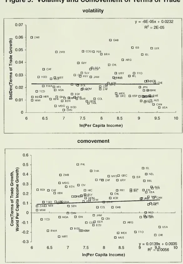
poor countries.

A

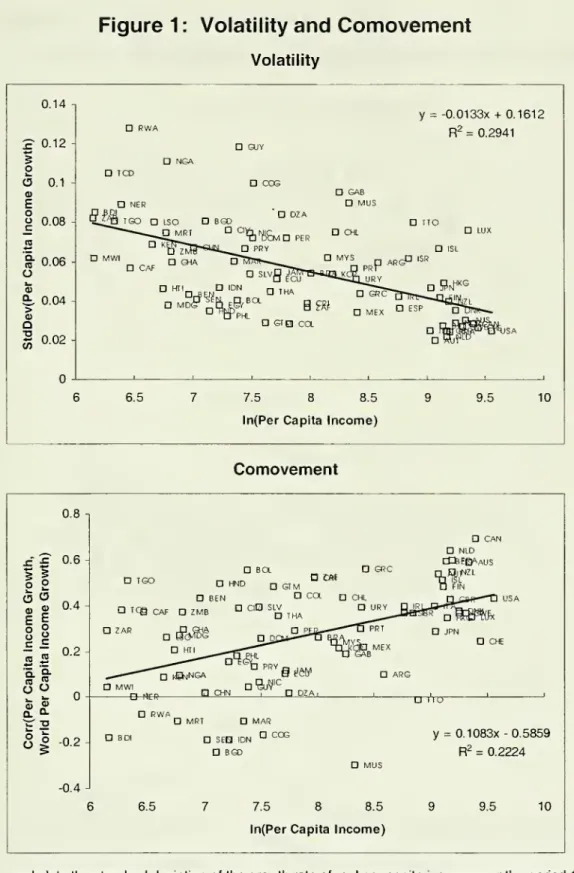
firstdifference

is thatfluctuations in per capita

income

growth are smallerin rich countries than in

poorones, in the top panelof Figure 1,

we

plotthe standarddeviation of per capita

income

growth against the level of (log) percapita

income

for a large

sample

of

countries.

We

referto this relationship asthevolatility graph

and

notethat it slopes

downwards.

A

second

difference isthat fluctuations in per capita

income

growth are

more

synchronizedwith the world cycle in rich countries than in poor ones. Inthe bottom panel of Figure 1,

we

plotthecorrelation of percapita

income

growth rates

with world average percapita

income

growth, excluding thecountry in question,

against the level of (log) percapita

income

forthe

same

set ofcountries.

We

referto

this relationship as the

comovement

graph

and

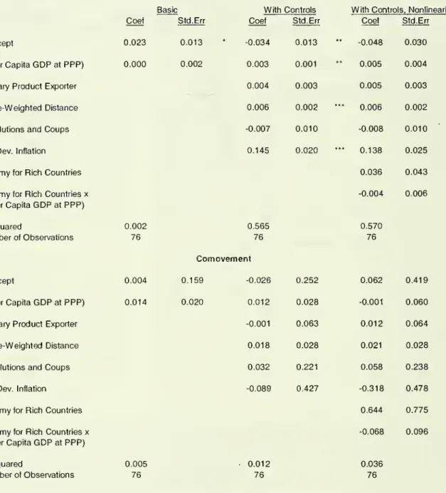
notethatit slopes upwards. Table 1

,

which is self-explanatory,

shows

thatthese facts applywithin different

sub-samples

of

countries

and

years.1

Why

are businesscycles less volatile

and

more

synchronized with theworld cycle in rich countriesthan in poor

ones?

Part ofthe

answer must be

that poor countries exhibit

more

political

and

policy instability, they are less

open

or

more

distantfromthe geographicalcenter,

and

they also

have

a highershare oftheir

economy

devoted tothe production of agricultural products

and

theextraction of minerals. Table 1

shows

that, ina statistical sense, thesefactors explain a substantial fraction of thevariation in thevolatility of

income

growth, althoughthey

do

not explain

much

ofthe variation in the

comovement

of

income

growth.

More

importantfor our purposes, the strong relationship

between income

and

the propertiesof business cycles reported in Table 1 is still present after

we

controlfor these variables. In short, there

must be

otherfactors behind the strong patterns depicted in Figure 1

beyond

differences in political instability,

remoteness

and

theimportance of natural resources.

Withthe exceptionthatthecomovementgraphseemsto bedriven bydifferencesbetween rich and

poorcountriesandnot within eachgroup.AcemogluandZilibotti (1997)alsopresent thevolatilitygraph.

Theyprovideanexplanationforitbased ontheobservationthatrichcountrieshavemorediversified

In this paper,

we

develop two alternative but non-competing explanationsfor

why

businesscycles are less volatile

and

more

synchronizedwith the world in rich

countriesthan in poor ones. Both explanations rely

on

the idea that comparative

advantage

causes

richcountries to specialize in industries that require

new

technologies operated by skilledworkers, while poorcountries specialize in industries that requiretraditional technologies operated by unskilled workers. This pattern of specialization

opens up

the possibilitythat cross-country differences in business

cycles are the result of

asymmetries

between

these typesof industries. In particular,

both ofthe explanations

advanced

here predict that industries that

use

traditional

technologies operated by unskilled workers will

be

more

sensitive to country-specific shocks. Ceteris paribus, these industrieswill not only

be

more

volatile but alsoless synchronizedwith the world cycle since the relative importanceof global shocks is

lower.

To

the extentthatthe business cyclesof countries reflectthose of their

industries, differences in industrial structurecould potentially explain the patterns in

Figure 1

.

One

explanation of

why

industries reactdifferentlyto

shocks

is

based on

the ideathatfirms using

new

technologies face

more

inelastic product

demands

than those using traditional technologies.

New

technologiesare difficultto imitate quickly

fortechnical reasons

and

also

because

of legal patents. This difficulty confersa cost

advantage on

technological leaders that shelters

them

from potential entrants

and

gives

them

monopoly power

inworld markets. Traditionaltechnologies are easierto

imitate

because

enough

time

has

passed

sincetheir adoption

and

also

because

patents

have

expired or

have

been

circumvented. This impliesthat

incumbent

firms face tough competition from potential entrants

and

enjoy little or

no

monopoly power

inworld markets.

The

price-elasticityof product

demand

affects

how

industries react to shocks.

Consider, for instance, theeffects of country-specific

shocks

that

encourage

production in all industries. In industries that

use

new

technologies, firms

have

monopoly power and

face inelastic

demands

for their products.

As

a result,

competition from

abroad and

therefore face elastic

demands

for their products.

As

a

result, fluctuations in supply

have

little or

no

effect

on

their prices

and

industry

income

is

more

volatile.

To

the extentthat this

asymmetry

in the

degree

of product-market

competition is important,

incomes

of industries that

use

new

technologies are likelyto

be

lesssensitive to country-specific

shocks

than those of industries thatuse

traditional technologies.

Another explanation for

why

industries react differentlyto shocks is

based on

the idea that the supplyof unskilledworkers is

more

elastic than the supplyof skilled

workers.

A

firstreason for this

asymmetry

is that non-market activities are relatively

more

attractive tounskilled workers

whose

market

wage

is lowerthan thatof skilled

ones.

Changes

in labour

demand

might induce

some

unskilledworkersto enteror

abandon

the labourforce, but are notlikelyto affect theparticipation of skilled

workers.

A

second

reason forthe

asymmetry

in labour supply across skill categories

is the imposition ofa

minimum

wage.

Changes

in labour

demand

might force

some

unskilledworkers in

and

outof

unemployment,

butare not likelyto affectthe

employment

of skilled workers.

The

wage-elasticityofthe labour supply also

has

implicationsfor

how

industries react toshocks. Consider again the effects of country-specific shocksthat

encourage

production in all industries

and

therefore raisethe labour

demand.

Since the supply of unskilledworkers is elastic,these shocks lead to large fluctuations in

employment

of unskilledworkers. In industries that

use

them,fluctuations in supply are therefore magnified by increases in

employment

that

make

industry

income

more

volatile. Sincethe supply of skilledworkers is inelastic, the

same

shocks

have

littleor

no

effects

on

the

employment

of skilledworkers. In industries that

use

them, fluctuations in supply are not magnified

and

industry

income

is less volatile.

To

the extentthatthis

asymmetry

in the elasticityof laboursupply is important,

incomes

of

industries that use unskilled workersare likelyto

be

more

sensitive to country-specific

shocks

than those of industries that use skilledworkers

To

studythese

hypotheses

we

constructa stylized world equilibrium

model

of the cross-section of business cycles. Inspired bythe

work

of Davis(1995),

we

consider insection

one

a world in which differences in both factor

endowments

a la

Heckscher-Ohlin

and

industrytechnologies a la Ricardo

combine

todetermine a country's comparative

advantage

and, therefore, the patterns of specialization

and

trade.

To

generate business cycles,

we

subjectthisworld

economy

to the sort of productivity fluctuations that

have

been

emphasized

by Kydland

and

Prescott (1982).2

Insection two,

we

characterize the cross-section of business cycles

and

show

how

asymmetries

in the elasticityof product

demand

and/or labour supply

can be

used

to explain the evidence in Figure 1. Using available

microeconomic

estimatesof the key

parameters,

we

calibratethe

model

and

find that: (i)

The

model

exhibits slightly less than two-thirds

and

one-third ofthe observed cross-country variation in volatility

and

comovement,

respectively;

and

(ii)

The

asymmetry

in the elasticityof product

demand

seems

to

have

a quantitatively stronger effect

on

theslopes of the volatility

and

comovement

graphs, than the elasticity in the labour supply.

We

explore these results further in sections three

and

four. In section three,

we

extendthe

model

to allow for

monetary

shocks

that

have

real effectssince firms facecash-in-advance constraints.

We

use

the

model

to study

how

cross-country variation in

monetary

policy

and

financial

development

affectthe cross-section of business cycles.

Once

thesefactorsare considered, the calibrated versionof the

model

exhibits roughly the

same

cross-countryvariation in volatility

and

about

40

percent of thevariation in

comovement

asthedata. In sectionfour,

we

show

that the two industry

asymmetries

emphasized

here lead toquite different implications forthe

cyclical behaviorof the termsof trade.

When we

confront these implicationswiththe

data, thepicture that

appears

isclear

and

confirms our earliercalibration result.

Namely, the

asymmetry

inthe

product-demand

elasticity

seems

quantitatively

more

importantthan the

asymmetry

in the labour-supplyelasticity.

2

Ourresearch isrelatedtothelarge literature onopen-economyrealbusinesscyclemodelsthat

studieshowproductivityshocks are transmittedacrosscountries.See Baxter (1995)and Backus,

Kehoeand Kydland (1995)fortwo alternativesurveysof thisresearch.

We

differfromthisliteraturein

two respects. Instead ofemphasizingtheaspects inwhich businesscycles aresimilaracrosscountries,

The

main

theme

of this paperis thatthe properties of business cycles differ

acrosscountries

because

they

have

differentindustrial structures.

There

are

many

determinantsof theindustrial structure of a country.

We

focus here

on perhaps

the

most

importantof

such

determinants, that is, a country's ability totrade. In section

five

we

explorefurtherthe connection

between

internationaltrade, industrial structure

and

the nature of businesscycles.

We

introducetrade frictions in theform of "iceberg"transport costs

and

study

how

globalization

(modeled

here as parametric reductions in transport costs)

changes

the nature of thebusiness cycles that

countries experience. Iftransport costs are high enough, all countries

have

the

same

industrial structure

and

the cross-section of business cycles is flat.

As

transportcosts

decline, the prices of products in which a countryhas comparative

advantage

increase

and

so

does

their share in production.

As

a result, industrial structures diverge.

One

shouldtherefore expect globalization to lead to business cyclesthat are

more

different acrosscountries.

1.

A

Model

of

Trade

and Business

Cycles

Inthis section,

we

present a stylized

model

ofthe world

economy.

Countries that

have

bettertechnologies

and

more

skilledworkersare richer,

and

alsotend to specialize in industries that use these factors intensively. Thatis, the

same

characteristics thatdeterminethe

income

of a country also determine its industrial

structure.

Our

objective isto develop a formal

framework

that allowsus to thinkabout

how

cross-countryvariation in industrial structure,

and

therefore income, translates

intocross-country variation in the propertiesof the business cycle.

We

considera worldwith a continuum ofcountries with

mass

one;

one

final

good and

two

continuums

of intermediates indexed by ze[0,1],which

we

refertoas the a-

and

(3-industries;

and

two factorsof production, skilled

and

unskilledworkers.

There

is freetrade in intermediates, but

we

do

not allowtrade inthe final good.

To

simplifythe

problem

further,

we

also rule out investment. Jointly, these assumptions imply that countries

do

notsave.

Countries differ in theirtechnologies, their

endowments

of skilled

and

unskilledworkers

and

their level of productivity. In particular,

each

country is defined

by atriplet (n,5,7t),

where

\iis

a

measure

of

how

advanced

thetechnology ofthe country is, 5is the fraction ofthe population that isskilled,

and

n is

an

index of productivity.

We

assume

thatworkers cannot migrate

and

that cross-country

differences in technology arestable, sothat \i

and

5are constant. Let F((i,5)

be

their

time-invariantjoint distribution.

We

generate businesscycles byallowing the productivity index

n

to fluctuate randomly.

Each

countryis populated by a

continuum

of

consumers

who

differ intheir

level of skills

and

their personal opportunity cost of work, or reservation

wage.

We

think ofthis reservation

wage

as thevalueof non-market activities.

We

index

consumers

by ie[1,»)

and

assume

thatthis index is distributed accordingto this

Pareto distribution: F(i)

=1-i

_x, with X>0.

A

consumer

with index i

maximizes

the

following expected utility:

(1) Ejufc(i)

WVe-.dt

o v

';

where

U(.) is

any

well-behaved utilityfunction; c(i) is consumption of thefinal

good

and

l(i) is

an

indicatorfunction thattakes value 1 if the

consumer

works and

otherwise. Let r(|i,5,7i)

and

w(fx,8,7t)

be

the

wages

ofskilled

and

unskilled workers in a

(H,5,7t)-country. Alsodefine _pF(n,8,7t) astheprice of the final good.

The

budget

constraint is simply p_F •_c(i)=

w

•l(i) for unskilledworkers

and

pF •c(i)= _r•_l(i) for

skilled ones.

The consumer

works

if

and

only ifthe applicable real

wage

(skilledor

unskilled)

exceeds

a reservation

wage

of i" 1

of skilled

and

unskilled workersthat are employed.

Under

theassumption that the

distribution of skills

and

reservation

wages

are independent,

we

have

that

(2) (3) f - \

vPf,

u

=

\ (1-5)

'w^

K^J

1-5

if r

<

_pF if r

>

_p F if

w

<

_pF if

w

>

_p F

Ifthe real

wage

of

any

type of workeris less than one, theaggregate labour supplyof this type exhibits awage-elasticityof X. This elasticity

depends

only

on

the dispersion of reservation

wages.

Ifthe real

wage

of

any

type ofworker reachesone,

theentire labour forceof this typeis

employed and

the aggregate laboursupply for thistypeof workers

becomes

vertical. Throughout,

we

consider equilibria in which the

x

real

wage

for skilled workers

exceeds

one,

—

>

1 , whilethe real

wage

forunskilled

Pf

w

workers is less than one,

—

<1 . That is, all countries operate in thevertical region

Pf

of their supplyof skilledworkers

and

the elastic region of theirsupplyof unskilled

workers. This assumption generates

an

asymmetry

inthe wage-elasticity of the aggregate laboursupply across skill categories. Thiselasticityis zero for skilled

workers

and

X>0

for unskilledones.

As

X-^0, this

asymmetry

disappears.

Each

country contains

many

competitivefirms in thefinal

goods

sector.

These

firms

combine

intermediatesto

produce

thefinal

good

according tothiscostfunction:

Thisisthecaseinequilibriumifskilled(unskilled)workersaresufficientlyscarce (abundant) inall

(4) B(p_a(z),p p(z))

=

V 1-v "1 M) "1 1-e

JPa(zr

dz

_Jp

P(z) 1- e dz _0 .0

The

elasticity ofsubstitution

between

industries is one, while theelasticityof

substitution

between any two

varieties within

an

industry is9, with 6>1

.

Sincethereare always

some

workersthat participatein the labourforce, the

demand

forthefinal product is always strong

enough

to generate positive production

in equilibrium.

Our assumptions on

technology implythatfirms in the final

good

sector

spend

a fraction vof their

revenues

on

a-products

and

a fraction 1-v

on

(3-products. Moreover, the ratioof spending

on

any

two a-products z

and

z' is given by

Pa(z) P.(z')

1-e

;

and

the ratioof spending

on

any

two (3-products z

and

z' is

Pp(z)

Pp(z')

1-e

where

pa(z)

and

p (z) denote theprice of varietyz of the a-

and

(3-products,

respectively. Define P_n

and

P

p asthe ideal price

indices forthe a-

and

(3-industry, i.e.

P

_a

=

Jp

a(z) 1- 9 -dz

and P

R =

Jp

p(z) 1- e -dz 1 1-e

;

and

define thefollowing

numeraire rule:

(5) 1

=

P«

v

-Pp"v

Sincefirms inthefinal

goods

sector are competitive, they set price equals cost. This implies that:

(6) pF

=1

Sinceall intermediates aretraded

and

the lawof

one

price applies, the price

power

parity applies.

An

implication of this isthat the

assumption

thatthe final

good

is nottraded is not binding.

Each

country also containstwo intermediate industries.

The

a-industry uses sophisticated production processes that require skilled workers.

Each

variety requires a differenttechnology that is

owned

by

one

firm only.

To

produce

one

unitof

any

variety ofa-products, thefirm that

owns

the technology requires

e"

units of skilled

labour.

As

mentioned, the productivityindexn fluctuates

randomly

and

is not under thecontrol ofthefirms. Let _n

be

the

measure

of a-productsin which thetechnology

is

owned

by a domestic firm.

We

can

interpret

_n

as a natural indicator of

how

advanced

the technologyof a country is. Itfollowsfrom our

assumptions on

the

technology

and

market structurein thefinal

goods

sector thattheelasticityof

demand

for

any

varietyof a-product is 0.

As

a result, allfirms in the a-industry face

downward-sloping

demand

curves

and behave

monopolistically. Their optimal pricing policyis to set a

markup

over unitcost. Let pjz) bethe price ofthevariety z of the a-industry.

Symmetry

ensures all thefirmslocated in a (|i,8,7i)-country setthe

same

pricefor theirvarieties of a-products, _p

a(ja,8,7r):

(7) paa =

re"

6-1

As

usual, the

markup depends on

the elasticityof

demand

for their products.

The

(3-industryuses traditional technologiesthat are available to all firms in all

countries

and can be

operated by both skilled

and

unskilledworkers.

To

produce one

unit of any varietyof (3-products firms require e" units of labourof

any

kind. Since

we

have

assumed

that inequilibrium skilled

wages

exceed

unskilled

wages,

only

unskilled workers produce (3-products. Sinceall firms in the (3-industry

have access

to the

same

technologies, they all faceflat individual

demand

curves

and behave

competitively.

They

set priceequal to cost. Let_p (z)

be

the price ofthevariety z of

the (3-industry.

Symmetry

ensures that all firms in the P-industryof a (n,5,7r.)-country

setthe

same

price forall varieties of _{(3-products, p^n,S,n):}

(8) p_p =w-.e-"

With this formulation,

we

have

introduced

an

asymmetry

in the price-elasticity of product

demand.

This elasticity is in the a-industry

and

infinity inthe (3-industry.

As

0^co

; this

asymmetry

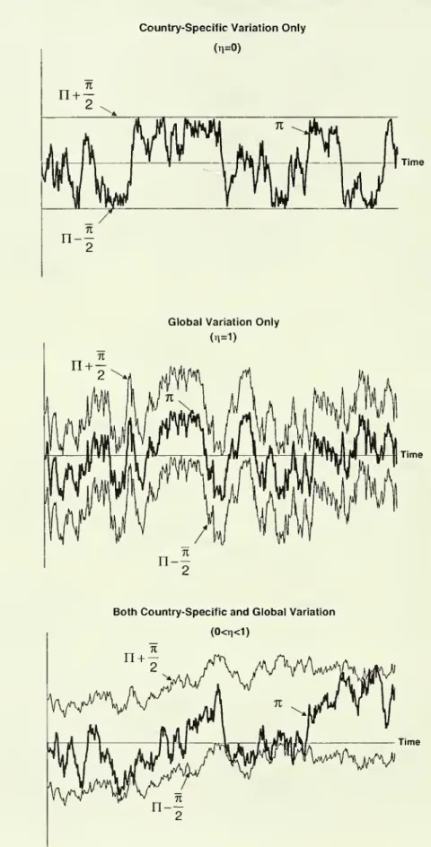
disappears.

Business cycles arise as

n

fluctuates randomly.

We

refer to

changes

in

n as

productivity shocks.

The

index

%

is the

sum

of a global

component,

n,

and

a country-specific

component,

n-Y\.

Each

of these

components

is

an

independent Brownian

motion reflected

on

the interval [-1,1] with

changes

that

have

zero drift

and

instantaneous variance equalto r\a2

and

(1-r|)rj2 respectively, with

%

>0, 0<r|<1

and

a>0. Letthe initial distribution of country-specific

components

be

uniformly distributed

on

[-n,7i]

and

assume

this distribution is independentof other country

characteristics.

Under

the

assumption

that

changes

in these country-specific

components

are independent across countries,

we

have

thatthe cross-sectional

distribution of 71-n istime invariant.4

We

refer tothisdistribution as G(7i-n). While

n

has

been

defined

as

an

index of domesticproductivity,

n

serves as

an

indexof world

average

productivity.

The

parameter

a

regulates thevolatilityofthedomestic shocks.

The

instantaneous correlation

between

domestic shocks, dn,

and

foreign shocks, dn,

is therefore Jr) .

5

The

parameter

ti therefore regulates the extentto which the

variation in domestic productivity is

due

to global or country-specific

components,

i.e.

whetherit

comes

from

dn

or d(7i-n). Figure 2

shows

possible

sample

paths_of

n

underthree alternative

assumptions

regardingt|.

4

SeeHarrison(1990),Chapter5.

Thisistrueexceptwheneithernor

n

areattheir respectiveboundaries.These arerareevents since

A

competitive equilibrium ofthe world

economy

consistsof a

sequence

of prices

and

quantities

such

that

consumers and

firms

behave

optimally

and

markets

clear.

Our assumptions

ensurethat a competitive equilibrium exists

and

is unique.

We

provethis byconstructing theset of equilibrium prices.

In thea-industry, different products

command

different prices.

The

ratio of

world

demands

forthe

(sum

of all) a-products of a (^,5,7i)-country

and

a

(n',d',n')-country,

—

P.W

,

must

equal the ratio of supplies is

se'

se

Pa(z')

condition plus Equation (2)

and

the definition of P

a

we

find that: . Usingthis (9) Pa

v

a

H

1 ^9 n-n

where

*¥„

=

IW

1 e-1

8

—

9 (n-n)

_dF-dG

v.

Since the distribution functions F(u.,8)

J

and

G(n-n) aretime-invariant, x

¥

_a is aconstant. Since

each

country isa "large" producer of its

own

varieties of a-products, the price ofthesevarieties

depends

negatively

on

the quantityproduced. Countrieswith

many

skilled workers (high 8)

with relatively high productivity (high 7i-n) producing a small

number

of varieties (low

|i) produce large quantitiesof

each

variety ofthe a-products

and

as a result, face low prices.

As

9^>°°, the dispersion in theirprices disappears

and

_p

ra(z)—>pa

.

Inthe (5-industryall products

command

the

same

price. Otherwise, low-price

varieties of (3-products would not

be

produced. Butthis is nota possible equilibrium given the technology described in Equation (4). Therefore, itfollows that:

(10) Pp

Finally,

we

compute

the relativeprice of both industries.

To

do

this, equate

v

the ratio of world spending in the a-

and

(3-industries, ,to the ratio of thevalue

1-v

ffp

_a

s-e"dFdG

of their productions,

^

. Using Equations _(2)-(3)

and

_(5)-(10),

we

j

jPpue

n

dFdG

then find that:

(11)

P

1 f v

%

\~

1-v

W

n 1+X.-V

—

-

—

n 1+Xv •e*

where

y

p

=

JJ(1-5)-e

(1+X)(n_n)

_dFdG

,

and

is constant. IfX>0, high productivity is

associated with high relative pricesfor a-products as theworld supplyof (3-products

is high relativeto thatof a-products. This increasein the relative supplyof (3-products

is

due

to increases in

employment

of unskilledworkers.

As

A.-^0, the relative prices of

both industries are unaffected bythelevel of productivity.

What

are the patterns oftrade inthisworld

economy?

Lety(n,§,7i)

and

x(n,5,Tr)

be

the

income

and

theshare of the a-industry in a (n,5,7i)-country, i.e.

/ \ d •s•o

71

y

=

(pa •s

+

pp

•

u}

e"

and

x

=

—

. Notsurprisingly, countrieswith better

technologies _{(high n)}

and

more

human

capital (high 5)

have

highvalues for both _y

and

x.

We

therefore refer to countries with high values ofx

as

rich countries. Since

each

country

produces an

infinitesimal

number

of varieties of a-products

and uses

all

of

them

in the production offinal goods, all countries exportalmost all of their

production of a-products

and

importalmost all of the a-products

used

in thedomestic production of final goods.

As

a

shareof income, these exports

and

imports are x

and

v, respectively.

To

balancetheir trade, countrieswith

x<v

export (3-products

and

v-x

and

x-v, respectively. Therefore, the share of trade in

income

is max[v,x].

As

usual, thistrade can

be

decomposed

into intraindustry trade, min[v,x],

and

interindustrytrade,Ix-v| .

The

former consistsof trade in productsthat

have

similar

factor proportions.

The

laterconsistsof trade in productswith different factor

proportions.

The

model

thereforecaptures in a stylized

manner

three broad empirical regularities regarding the patterns of trade: (a) a large

volume

of intraindustry trade

among

rich countries, (b) substantial interindustrytrade

between

rich

and

poor

countries,

and

(c) littletrade

among

poorcountries.

2.

The

Cross-section

of

Business

Cycles

Inthe world

economy

described in the previoussection, countries are subject

tothe

same

type of country-specific

and

global

shocks

to productivity.

Any

difference

in the properties oftheir business cycles

must be

ultimately attributed to differences

in theirtechnology

and

factorproportions. This is clearly asimplification. Inthe real

world countriesexperience differenttypesof

shocks

and

also differ in

ways

that

go

beyond

technology

and

factor proportions. With thiscaveat in mind, in this section

we

ask:

How

much

of the observed cross-countryvariation in business cycles could potentially

be

explained bythesimple

model

of theprevious section?

Perhaps

surprisingly, the

answer

is

between

one

and

two thirds ofall the variation.

The

first steptowards answering this question isto obtain

an

expression that

links

income

growth tothe shocksthat countries experience. Applying Ito's

lemma

to

the definition of y

and

using Equations (2)-(11),

we

obtain the

(demeaned)

growth

rate of

income

ofa (n.,5,7t)-country

as

a

linearcombination of country-specific

and

global shocks: (12)

dlny-E[dlny] =

x-

—

+(1-x)-(1+X)

d(7t-n)+

1+ x

dn

1+X-v

15

Equation (12) provides a complete characterization ofthe businesscycles experienced by a (u.,5,7i)-countryas afunction ofthe country's industrial structure,

as

measured

byx. Equation (12)

shows

that poorcountries are

more

sensitive to

3dlny

country-specific shocks, i.e.

ad(Ti-n)

is decreasing in x. Equation (12) also dn=o

shows

thatall countries are equally sensitive to global shocks, i.e

adn

independentof x.

We

nextdiscuss the intuition behind these results.

is d(;t-n)=o

Why

are poorcountries

more

sensitiveto country-specific

shocks?

Assume

that

X-^0

and

9^°°

>

so

thatthe

a-and

(3-industryface both perfectly inelasticfactor

supplies

and

perfectly elasticproduct

demands.

Inthiscase, a

one

percent country-specific increase in productivity

has

noeffects on

employment

or product prices.

As

a

result, production

and income

also increase by

one

percent. This is

why

3dlny

ad(Ti-n)

=

1 if A.-^0

and

6^^.

If A,is positive, a country-specific increase in

dn=o

productivityof

one

percent leadsto

an

increase in

employment

of A. percent in the

(3-industryand, as a result, production

and income

increase by

more

than

one

percent. This

employment

response magnifiesthe expansionary effects of increased

productivity in the (3-industry.

As

a result, the

shock

has

stronger effects in poor 3dlny

countries, i.e.

3d(7t-n)

=

1

+

(1—x)-A, if

8—

>°°. If6 is finite, a country-specific dn=o

increase in productivity of

one

percent leads toa 0"1

percent

decrease

in prices inthe

a-industries. Thisprice

response

counteracts the expansionaryeffects of increased productivity inthea-industry. Consequently, the

shock

has

weaker

effects in rich

Bdlny countries, i.e.

x

=

1

—

ifX=0. If

X>0 and

9 isfinite,

we

have

that both the

employment

and

price

responses combine

to

make

poor countries react

more

to

country-specific shocks, i.e.

dd(Ti-n)

—

1

=

x

+

(1-x) (1

+

X) is decreasing in x.

Why

areall countries equally responsiveto global

shocks?

This result rests

on

theassumption thattheelasticity of substitution

between

a-

and

(3-productsis

one. Consider a global increase in productivity.

On

the

one

hand, production of p-products

expands

relativeto the production of a-productsas

more

unskilled workers are employed. Ceteris paribus, this

would

increase the share ofworld

income

that

goes

tothe p-industry,

and hence

poorcountries, aftera positive global shock. But theincrease in relative supply lowers the relative price of p-products. This reduces theshare ofworld

income

that

goes

to the P-industry,

and hence

poorcountries, after a positive global shock.

The

assumption

ofa

Cobb-Douglas

technologyforthe

production ofthe final

good

implies that thesetwoeffectscancel

and

theshare of

world spending in the a-

and

P-industries remains constant overthe cycle. Therefore,

in our

framework

differences in industrial structure

do

notgenerate differences in

how

countries react to global shocks.6

We

are readyto

use

the

model

to interpretthe evidence in Figure 1. Define

dlnY

as

theworld average growth rate, i.e.

dlnY =

jj dlny

dFdG

. Then, it follows

from Equation (12) that:

(13)

dlnY-E[dlnY]

=

1

+

X

dn

1

+ A-v

Sincethe lawof large

numbers

eliminates the country-specific

component

of

shocks

in the aggregate, the world

economy

exhibits mildercyclesthat

any

ofthe countriesthat belong to it.

7

6

WhiletheCobb-Douglasformulation isspecial, itisnotdifficulttograsp whatwould happenifwe

relaxed it. Iftheelasticity ofsubstitutionbetween industrieswerehigherthan one, poorcountrieswould

be moresensitivetoglobalshocksthanrichcountriesastheshareofworld incomethatgoestothe

|3-industry increasesafterapositiveglobalshock and decreasesafteranegative one. Iftheelasticity of substitutionwere lessthan one, the oppositewould betrue.

7

Once again,this resultrestsontheCobb-Douglas assumption. Iftheelasticityofsubstitutionbetween

a-and|3-productswere higherthan one, the very richcountries mightexhibitbusinesscyclesthatare

milderthan thoseoftheworld.

Let V(n,8,7i)

denote

the standarddeviation of

income

growth of a

(u.,5,7t)-country,

and

let CQx,5,7c)

denote

thecorrelation of its

income

growth with world

average income

growth.

These

are the theoretical analogs to thevolatility

and

comovement

graphs

in Figure 1. Using Equations (12)-(13)

and

the propertiesofthe

shocks,

we

find that:

(14)

V

=

o-. (15)

C

=

x

.^I

+

(1-x)-(1

+

X) -i2 (1"T1)+ '

^+x

^ -\

+ X-v

1

+

1-v

f\

x

.®^

+

(1-x)-(1

+

X) •(1-71)

+

1

+ A

1

+ X-v

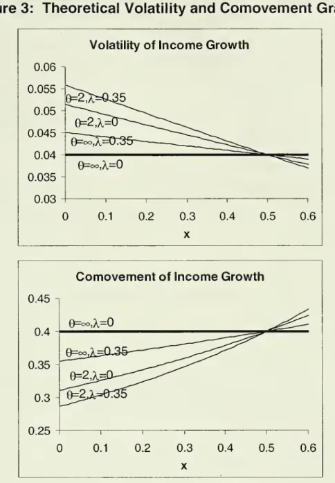
Tl

Figure 3 plotsthe volatility

and

comovement

graphs

asfunctionsof x, for

differentparameter values. Exceptin the limiting

case where

both

X=0

and

0=<~, the

volatilitygraph is

downward

sloping

and

the

comovement

graph is

upward

sloping.

The

intuition is clear:

As

a result of

asymmetries

in theelasticity of

product-demand

and

labour supply, the a-industryis less sensitive to country-specific

shocks

thanthe

(3-industry. This

makes

the a-industry lessvolatile

and

more

synchronizedwith the

world cyclethan the (3-industry. Sincecountries inherit the cyclical properties of their

industries, the

incomes

of rich countries are also lessvolatile

and

more

synchronized with the world cyclethan thoseof poorcountries.

The

magnitude

of these differences

is

more

pronounced

as

X

increases and/or 6 decreases.

A

simple inspection of Equations (14)

and

(15) revealsthat there existvarious combinations of

parameters

capable of generating approximatelythe data patterns displayed in Figure 1

and

Table 1. Inthis sense, the

model

is able to replicate the

evidencethat motivated the paper. Butthis is a very

undemanding

criterion.

One

can

impose

more

discipline

by

restrictingthe analysis tocombinations of parameter values that

seem

reasonable.

To

do

this,

we

next

choose

valuesfor a, r\, v

and

a

businesscycles varies with X

and

9. Needlessto say,

one

should

be

cautious to

draw

strong conclusionsfrom a calibration exercise likethis in a

model

asstylized

as

ours.

As

noted above, in the realworld countries experience differenttypesof

shocks

and

alsodiffer in

ways

that

go beyond

technology

and

factorproportions. Moreover,

availableestimates of the key parameters

X

and

9are

based on

non-representative

samples

ofcountries

and

industries, sothat caution is in order

when

generalizing to the largecross-section of countries

we

study here. Despite these caveats,

we

shall

see that

some

useful insights can

be

gained fromthis exercise.

To

determinethe relevant rangeof variationforx,

we

use data

on

trade shares.

The

model

predicts thatthe share of exports in

income

in rich countries is x.

Sincethis share is

around 60

percent inthe richest countries in our sample,

we

use

0.6 as a reasonable upper

bound

for x.

The

model

also predicts that v is theshare of exports in

income

in poor countries,

and

that in these countries x<v. Sincethe share

of exports in

GDP

is

around 20

percent inthe poorestcountries in oursample,

we

choose

v=0.2

and

use0.1 as alower

bound

forx.

The

choice ofrj

and

r\ is

more

problematic, since there are

no

reliableestimates of the volatility

and

cross-country correlation of productivitygrowth for this large cross-section of countries.

We

circumventthis

problem

by choosing

a and

r| to

match

theobserved level of volatility

and

comovement

of

income

growthforthetypical rich country, given the rest of our parameters.8 This

means

thatthis calibration exercise

can

only tell us aboutthe

model's abilityto

match observed

cross-country differences involatility

and

comovement

of

income

growth.

The

top-left panel ofTable 2 reportsthe resultsof this calibration exercise,

and

selected

cases

are

shown

in Figure 3.

The

first row reportsthe predicted difference in volatility

and

comovement

between

the richest country(with log per capita

GDP

of around 9.5)

and

the poorestcountry (with log percapita

GDP

of around 6.5),

based on

the regressionswith controls in Table 1.

The

remaining

rows

In particular,a andr|arechosentoensurethatV=0.04 andC=0.4,forx=0.5,v=0.2andthe given

choicesforAand9.

report the difference involatility

and

comovement

between

the richest (x=0.6)

and

poorest (x=0.1) countries thatthe

model

predicts fordifferent valuesof

X

and

0.

These

values

encompass

existing

microeconomic

estimates. Available industry estimates ofthe elasticity of export

demand

range from 2to 10 (see Trefler

and

Lai (1999), Feenstra, (1994)), whileavailable estimatesforthe labour supply elasticity of

unskilled workers range from 0.3 to 0.35

(See

Juhn,

Murphy and

Topel (1991)).

The

table also reports thevaluesfor

a

and

r\that resultfrom the calibration procedure.

Table 2

shows

that, using values for8

and

X of

9=2 and

A.=0.35, the

model

can accountfor nearlytwo-thirds ofthe cross-country difference in volatility

between

rich

and

poorcountries (-0.016versus -0.026),

and

slightly lessthan one-third ofthe cross-country differences in

comovement

(0.129 versus 0.382).

These

values forthe parameters are within the range

suggested by

existing

microeconomic

studies. Ifthe

industry

asymmetries

are

assumed

to

be even

stronger, say 9=1.2

and

X=0.7, the predicted differences in volatility

and

comovement

are closerto their predicted values.

These

results

seem

encouraging.

The

two

hypotheses put forward here

can

accountfora sizeable fraction of cross-country differences in business cycles

even

in

such

a stylized

model as

ours. Moreover,

we

shall

see

in the next section that a simple extension ofthe

model

that allowsfor

monetary shocks

and

cross-country differences in the

degree

offinancial

development

can

move

thetheoretical predictions closerto the data.

A

second

resultin Table 2 isthatthe

asymmetry

in theelasticity of product

demand seems

quantitatively

more

importantthan the

asymmetry

in theelasticity of

the labour supply. Within the range of

parameter

values considered in Table2,

changes

in 9

have

strong effects

on

the slopeof the two graphs, while

changes

in

X

to

have

little or

no

effect.

To

the extentthatthis range of parameter values

we

consider is the relevant one, this calibration exercise suggeststhat the

asymmetry

in

asymmetries

in the elasticity of product

demands

constitutesthe

more

promising hypothesisof

why

business cycles are different across countries.

We

return to this

point in section four

where

we

attemptto distinguish

between hypotheses by

3.

Monetary

Shocks and

Financial

Development

Our

simple calibration exercise tells us thatthe two industry

asymmetries

can

account for almosttwo-thirds of the cross-country differences in volatility,

and

nearly one-third ofthe cross-country variation in

comovement.

One

reaction tothisfinding is

thatthe

model

is surelytoo stylized to

be

confronted with the data. Afterall,

most

of our modelling choices

were

made

to

maximize

theoretical transparency ratherthan

model

fit.

Now

thatthe main

mechanisms

have

been

clearlystated

and

the intuitions

behind

them

developed, it is timeto build

on

the stylized

model

and

move

closerto

reality by adding details. This is the goal of this section,

where

we

show

thatby

introducing

monetary

shocks

and

cross-countryvariation infinancial

development

helps to significantlynarrowthe

gap

between model and

data. This is not the only

way

to narrow this gap, but

we

choose

to followthis route

because

the elementsthat

this extension highlights areboth realistic

and

interesting in their

own

right.

We

now

allow countriesto differalso in theirdegree offinancial

development

and

their

monetary

policy.

Each

country is therefore defined by a quintuplet,

(|j.,5,7:,k,i),

where

k is a

measure

ofthe

degree

of financial development,

and

i isthe interest rate

on

domestic currency.

We

assume

thatk is constant over time

and

re-define F(^,5,k) asthe time-invariantjointdistribution of \i, 8

and

k.

We

allowfor

an

additional source of business cyclesby letting ifluctuate randomly.

We

motivate the use of

money

by

assuming

thatfirms facea cash-in-advance constraint.9 In particular, firms

have

to

use cash

or domestic currency in orderto

pay

afraction k of their

wage

bill before production starts, with

0<k<1

.

The

parameter

k

therefore

measures

how

underdeveloped are credit markets.

As

k^O

in all countries,

we

reach the limit inwhich credit marketsare so efficientthat

cash

is neverused.

SeeChristiano,Eichenbaum andEvans (1997)fora discussionof relatedmodels.

This is the

case

we

have

studied so far. In thosecountries

where

k>0, firms borrow

cash

from the

government

and

repaythe

cash

plus interest after production is

completed

and

output is sold to

consumers.

Monetary

policy consists of settingthe interest rate

on cash

and

then

distributing the proceeds in a

lump-sum

fashion

among

consumers.

As

is

customary

in the literature

on

money

and

business cycles,

we

assume

that

monetary

policy is

random.

10 In particular,

we

assume

thatthe interest rate is a reflecting Brownian motion

on

the interval [i,T], with

changes

that

have

zerodrift, instantaneous

variance §2,

and

are independent acrosscountries

and

also independentof

changes

in n. Letthe initialdistribution of interest rates

be

uniform in [t,T]

and

independentof

the distribution of othercountry characteristics. Hence, the cross-sectional distribution of i, H(i),

does

not

change

overtime.

The

introduction of

money

leads onlyto minor

changes

in thedescription of

world equilibrium in section one. Equations (2)-(3) describing the labour-supply

decision

and

the numeraire rule in Equation (5) still apply. Sincefirms in thefinal

sector

do

not

pay

wages,

their pricingdecision is still given by Equation (6).

The

cash-in-advance constraintsaffect thefirms in the a-

and

(3-industriessince they

now

face financing costs in addition to labour costs.

As

a result, the pricing equations (7)-(8)

have

to

be

replaced by:11

(16) pa

=—

-r-e-™

e-1

(17) pp

=w-e"

10

Thissimplification isadequate ifonetakes the viewthatmonetarypolicy hasobjectivesotherthan

stabilizingthecycle. Forinstance,iftheinflationtaxisusedtofinancea publicgood, shockstothe

marginal valueof thispublicgoodare translatedintoshockstotherateofmoneygrowth. Alternatively,if

acountryiscommittedtomaintainingafixed parity,shockstoforeign investors'confidence inthe

country aretranslatedintoshockstothe nominalinterestrate, asthe monetaryauthoritiesusethe latter

tomanagetheexchangerate.

11

Note that

changes

in theinterest rate affectthe financing costs of firms

and

are therefore formally equivalenttosupplyshocks such as

changes

in production or payroll taxes. Formally, this isthe only

change

required.

A

straightforward extension

of earlier

arguments

shows

that Equations(9)-(11) describing the set of equilibrium

prices arestill valid provided

we

re-define

T

p =

J||(1-5)e

(1+A)(7t"_n)"Kl

dFdGdH,

which converges to the earlier definition of

Y

B inthe limiting

case

in which k-^0 in all

countries.

Financing costs are not a directcost forthe country

as

a

whole

but only a transferfrom firms to

consumers

via the government. Consequently,

income

and

the

/ \ p -s-e"

shareof the a-industry are still defined

as

y

=

\pa s

+

pp

•u) e

and

x

=

—

,

respectively.

Now

rich countries arethosethat

have

bettertechnologies (high _n),

more

human

capital (high 5)

and

better financial

systems

(low k).

Remember

that,

ceterisparibus, a highvalue for u.

and

S lead to a high valueof x. This is

why

have

been

referring tocountries with high values for xas rich.

However,

we

have

now

that a low valuefor k leads to both higher

income and

a lower value for x.

The

intuition is

simple:

A

high valueof k is associatedwith higher financing costs

and

thereforea

weaker

labour

demand

forall typesof workers. Inthe market for skilledworkers, this

weak

demand

is translated fully into low in

wages

and

has

no

effects in employment.

The

size of the a-industry istherefore notaffected by cash-in-advance constraints. In

the marketfor unskilled workers,this

weak

demand

is translated into both lower

wages

and employment.

The

latter implies a smaller (3-industry. Despite this,

we

shall

continueto referto countries with highervalues ofxas rich. That is, it

seems

tous

reasonable to

assume

thattechnology

and

factor proportionsare

more

important determinantsofa country's industrial structurethan the

degree

offinancial development.

We

are readyto determine

how

interest-rate

shocks

affect

income

growth

and

the cross-section of businesscycles. Applying Ito's

lemma

tothedefinition ofy,

we

find this expression forthe

(demeaned)

growth rate of

income

forthe (|n,5,7t,K,i)-country: (18) dlny-E[dlny]= x

.®-l

+

(1-x)-(1

+

X)

d(7t-n)+

1+

dn-(1-x)A-K-di

J \

+

Xv

Equation (18), which generalizes Equation (12), describes the business cycles of a (|j,,S,7i,K,i)-country

as

a

function of its industrial structure.

The

first

two

terms

describe the reaction of thecountryto productivity

shocks

and have

been

discussed at length.

The

third term is

new

and

shows

how

the country reactsto interest-rate shocks. In particular, it

shows

that interest-rate

shocks

have

largereffects in

countriesthatare poor

and have

a low

degree

offinancial development. That is,

3dlny 9di

is decreasing in x

and

increasing in k (holding constantx). d(rc-n)=o

dn=o

An

increase in the interest rate raisesfinancing costs in the a-

and

(3-industries. This increase is larger in countries with low

degrees

offinancial

development

(high k). Just

because

ofthis, poorcountries are

more

sensitive to interest-rate

shocks

than rich countries. But there is more. Inthe a-industry,the supply of labour is inelastic

and

the additional financing costs are fully

passed

to

workers in theform of lower

wages.

Production is therefore notaffected. Inthe

f3-industry, thesupplyof labour is elastic

and

theadditional financing costs are only

partially

passed

to

wages.

Employment

and

production thereforedecline. In the

aggregate, production

and income

decline after a positive interest-rate shock. But if

the

asymmetry

in the laboursupply elasticity is important, this reaction should

be

stronger in poorcountries that

have

larger (3-industries. This provides a

second

reason

why

poorcountriesare

more

sensitiveto interest-rate shocks than rich

countries.

The

introduction of interest-rate

shocks

provides two additional reasons

why

through their industrial structure

and

anotheris a

consequence

of their lack of

financial development. Both of theseconsiderations reinforcethe results of the

previous model.

To

see

this, re-define

dlnY =

f

|fdlny

dFdGdH.

Equation (13) still

applies since

monetary

shocks

arecountry-specific

and

the lawof large

numbers

eliminatestheir effectsin the aggregate. Then, rewrite the volatility

and

comovement

graphs asfollows: (19)

V=

a

2 (20)

C

=

a

2 .

x-iLl

₊

(1-x).(1

+

A.) (1-T1)

+

1+X

f 1 +

x

^ \ 1

+ X-v

1

+

X-v

2 12 Tl

+r-K^-(i-xr-A.'

x

.8_1

+(1_x).(1+X) (1-tl)

+

'

_1+X

^ 1

+

X-v

2 ,,-2 I* „\2 t2 •Tl

+r-K^-(1-Xr-X'

j

These

equations are natural generalizations of Equations (14)-(15).

They

show

that, ceteris paribus, countrieswith lowfinancial

development

will

be

both

more

volatile

and

less correlated with the world.

They

also

show

the

new

channel through

which industrial structure affectsthe business cycles ofcountries.

With these additionalforces present, the

model

is

now

ableto

come much

closertothe observed cross-countryvariation involatility

and

comovement

using values for9

and X

that are consistentwith available

microeconomic

studies. This is

shown

in the bottom panelof Table 2,

where

we

assume

thatthe standard deviation of

shocks

to

monetary

policy is 0.1

and

thatk=1 in the poorest countries in our

sample and

k=0.5 in the richest countries. For

9=2 and

X=0.35, the extended

model

now

delivers cross-country differences in volatilitythatare nearly identical tothe

ones

we

estimated in Table 1 (-0.024versus -0.026),

and

cross-country differences in

comovement

are

now

40

percentof those

we

observe in reality(0.165 versus 0.382). Looking further

down

thetable,

we

can further improvethe fitof the

model

in the

comovement

dimension byconsidering

more

extreme parametervalues.

However,

this is achievedat the cost of over-predicting cross-country differences in volatility.

We

could tryto furthernarrowthe

gap between

theory

and

databy

considering additional extensions to the model. But

we

think thatthe results obtained sofar are sufficientto establish that thetwo hypotheses considered here

have

the potential to explain at least in part

why

business cycles are different in rich

and

poor countries. This isour simple objective here.

4.

The

Cyclical

Behavior

of

the

Terms

of

Trade

From

the standpoint of the evidence reported in Table 1

and

the theory

developed in the previous sections, the two industry

asymmetries

studied hereare observationally equivalent.

However,

using

microeconomic

estimates for9

and X

as additional evidence to calibrate the model,

we

found that the

asymmetry

in the

elasticityof product

demand

seems

a

more

promising explanation of

why

business

cycles aredifferent across countriesthan the

asymmetry

in theelasticity of the labour supply. Inthis section,

we

show

that thesetwo

asymmetries have

different

implications forthe cyclical properties of theterms of trade,

and

then confronting these implications with thedata.

The

evidence

on

thecyclical behavior of theterms of

trade is consistent with the results ofour calibration exercise. Namely, a strong

asymmetry

inthe elasticityof product

demand

helps the

model

provide a

more

accurate description of theterms oftrade datathan a strong

asymmetry

in the

elasticityof the labour supply.

We

firstderivethe stochastic process forthetermsof trade.Let T((i,5,7t,k,i)

denote the

terms

of trade of a (|a,5,7r,K,i)-country. Using Equations (9)-(11),

we

find

thatthe (detrended) growth rate in theterms of trade is equalto:12

12

Itispossibletodecomposeincomegrowthintothegrowth ratesofproductionandtheterms oftrade.

Thegrowth rateofproduction(or

GDP

growthrate)measuresincomegrowththat isdueto changesin

production, holding constantprices.Thegrowthrate ofthetermsoftrademeasuresincome growththat

isduetochanges in prices,holdingconstant production.

We

followusualconvention anddefinethe

termsoftradeofa countryasthe ideal priceindexofproductionrelativetotheideal price indexof

expenditure.Thegrowth rateofthetermsoftradeisequaltotheshareofexportsin incometimesthe

(21)

dlnT-E[dlnT] =

--d(7i-n)+

(X v

^

-dn

9 1

+ A-V

Equation (21) describes thecyclical behaviorof thetermsof trade as

a

function ofthe country's industrial structure. It

shows

that positive country-specific

shocks

to productivity affect negativelytheterms of trade,

and

thiseffectis larger (in

adlnT

absolute value) the richer is the country, i.e. is negative

and

dn=o ad(Tt-n)

decreasing in x. Equation (21) also

shows

that positiveglobal

shocks

to productivity

worsen

the termsof trade of poor countries

and

improve thoseof rich countries, i.e. ~\f-iI—

T

is negative if

x<v

and

positive ifx>v. Finally, Equation (21)

shows

that

d(n-n)=0

adn

interest-rate shocks

have no

effects

on

theterms of trade.

We

discusstheintuition

behind these results in turn.

Country-specific

shocks

to productivity

have no

effecton import prices

because

countries are small. But they

do

affectexport prices. Consider a positive country-specific

shock

to productivity. In the a-industry, firms react to the

shock

by producing

more

of

each

variety they

know

how

to produce. Sincethis set is small, the increase inthe production of

each

varietyis large. Since domestic

and

foreign

varietiesare imperfect substitutes, the increase in production lowers the price ofthe country's a-products. Inthe P-industry, firms

know

how

to produceall varieties.

They

react tothe

shock

byspreading their production

among

a large

number

ofvarieties

(or byforcing

some

firms abroad to

do

this).

As

a result, the increase in the production of

each

varietyis infinitesimally small

and

theprices of the country's p-products are not affected. In the aggregate, theterms of trade

worsen

as a result of

the shock. But if the

asymmetry

in theelasticity of product

demand

is important, the termsof trade shoulddeteriorate

more

in rich countries.

Global shocks influence all countries equally and, consequently, they

do

not affect the prices ofdifferentvarieties of a-

and

P-products relativeto their

corresponding industryaggregates. Consider a positive global

shock

to productivity.

We

saw

earlierthatthis

shock

lowers the price of all (3-products relative to all

a-products

(See

Equation (11)).

The

reason is simple: In both industries, the increase

in productivity leads to a directincrease in production. But if the

asymmetry

in the

elasticity ofthe labour supply is important, the increase in productivity raises

employment

of unskilled workers

and

leads to afurther increase in theproduction of

(3-products.

As

theworld supplyof (3-products increases relative to that of a-products,

their relativeprice declines. This is

why

theterms oftrade of net exporters of

|3-products, x<v, deteriorate, while theterms oftrade of net importers of p-products, x>v, improve.

Finally, Equation (21) states that country-specific interest-rate

shocks

have no

effects

on

theterms oftrade.

These

shocks

do

not affect import prices

because

the country issmall. Butthey

do

not affect export prices either.

As

discussed earlier,

interst-rate

shocks

do

not affect the production of a-products.

As

a result, they

do

not affect theprices ofdomesticvarieties relativeto the industryaggregate. Interest-rate

shocks

affect the production of (3-products.

However,

firms in the p-industrycannot

change

their prices intheface of perfectcompetition from firms abroad.Therefore, country-specific

monetary

shocks

do

notaffect the termsof trade.

Equation (21)

makes

clear

how

thetwo industry

asymmetries

shape

the

cyclical behaviorofthe terms oftrade. Inthe

absence

of

asymmetries

in the elasticity

ofthe labour supply,

A—

>0, only country-specific

shocks

affectthe

terms

oftrade. In

the

absence

of

asymmetries

in the elasticityof product

demand,

8-^°=, only global

shocks

affect theterms of trade. This

has

implications forthevolatility

and

comovement

graphs fortheterms of trade. Let

V

T(fi,5,Tr,K,i)

denote

the standard deviation of the(detrended) growth of termsof trade of a (|a,8,7t,K,i)-country,

and

let

C

J(\i,5,n) denote its correlation with world

average

income

growth. Using Equations

(22)

V

T

=a-.

(23)

C

T = (1-il)+ V

(x-v)-A

1

+

A.v

Tl "l

+

X-v

V?

'ix-v)X^

fl-<1-1>

+

1

+

X-v

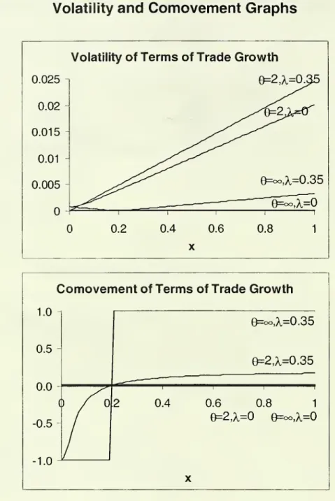
•Tl

To

understandthe intuition behind theseformulae, it is useful toconsidertwo

extreme

cases. Both are illustrated in Figure 4, which plots the volatility

and

comovement

graphsof theterms oftrade asfunctions of x, fordifferent parameter values.

Assume

firstthatthe only reason

why

business cycles differacross countries

isthe

asymmetry

in the elasticityof product

demand,

i.e. A=0.Then,

V

T

=

—

•

a

_•y/l-'n

and

C

T

=

.

The

volatilitygraph is

upward

sloping. Sinceall the

G

volatility in prices is

due

to

changes

in thedomestic varieties of a-products, the terms of trade are

more

volatile in rich countries

where

theshare ofthe a-industry is large.

The

comovement

graph isflat at zero. Whilethe termsof trade respond onlyto country-specific shocks, world

income

responds onlyto global shocks.

As

a result

both variablesare uncorrelated.

Assume

nextthat the only reason

why

business cycles are differentacross

countries is the

asymmetry

in the elasticityofthe labour supply, i.e. 0^><». Then, T lx-v|-X i— T 1-1 if x <v

V

=J !

cr-AH

an

d

C

=

i .

The

volatilitygraph looks like

a

V, with

1+

A.v

[ 1 if x

>

v

a

minimum

when

x=v. Since all the volatility in prices is

due

to

changes

inthe

aggregate industry prices, theterms oftrade are

more

volatile in countries

where

the share of interindustrytrade in overall trade is large, i.e. | x-v|is large.

These

are the

very rich

and

very poorcountries

whose

factor proportions

and

technology differthe

most

fromworld averages.

The

comovement

graph is a step function with a single step atx=v. Since global

shocks

driveboth the world cycle

and

theterms oftrade, these variablesare perfectly correlated. Ifthe country is a netexporterof a-products,