Conformal loop ensembles: the Markovian characterization and the loop-soup construction

Conformal loop ensembles: the Markovian

characterization and the loop-soup construction

The MIT Faculty has made this article openly available. Please share

how this access benefits you. Your story matters.

Citation Sheffield, Scott, and Wendelin Werner. “Conformal loop ensembles: the Markovian characterization and the loop-soup construction.” Annals of Mathematics 176, no. 3 (November 1, 2012): 1827-1917.

As Published http://dx.doi.org/10.4007/annals.2012.176.3.8

Publisher Princeton University Press

Version Original manuscript

Citable link http://hdl.handle.net/1721.1/80824

Terms of Use Creative Commons Attribution-Noncommercial-Share Alike 3.0

arXiv:1006.2374v3 [math.PR] 28 Sep 2011

Conformal loop ensembles:

the Markovian characterization and the loop-soup

construction

Scott Sheffield

_{and Wendelin Werner}

Abstract

For random collections of self-avoiding loops in two-dimensional domains, we define a simple and natural conformal restriction property that is conjecturally satisfied by the scaling limits of interfaces in models from statistical physics. This property is basically the combination of conformal invariance and the locality of the interaction in the model. Unlike the Markov property that Schramm used to characterize SLE curves (which involves conditioning on partially generated interfaces up to arbitrary stopping times), this property only involves conditioning on entire loops and thus appears at first glance to be weaker.

Our first main result is that there exists exactly a one-dimensional family of random loop collections with this property—one for each κ_{∈ (8/3, 4]—and that} the loops are forms of SLEκ. The proof proceeds in two steps. First, uniqueness

is established by showing that every such loop ensemble can be generated by an “exploration” process based on SLE.

Second, existence is obtained using the two-dimensional Brownian loop-soup, which is a Poissonian random collection of loops in a planar domain. When the intensity parameter c of the loop-soup is less than 1, we show that the outer boundaries of the loop clusters are disjoint simple loops (when c > 1 there is a.s. only one cluster) that satisfy the conformal restriction axioms. We prove various results about loop-soups, cluster sizes, and the c = 1 phase transition.

Taken together, our results imply that the following families are equivalent: 1. The random loop ensembles traced by branching Schramm-Loewner

Evolu-tion (SLEκ) curves for κ in (8/3, 4].

2. The outer-cluster-boundary ensembles of Brownian loop-soups for c_{∈ (0, 1].} 3. The (only) random loop ensembles satisfying the conformal restriction

ax-ioms.

∗_{Massachusetts Institute of Technology. Partially supported by NSF grants DMS 0403182 and DMS}

0645585 and OISE 0730136.

†_{Universit´e Paris-Sud 11 and Ecole Normale Sup´erieure. Research supported in part by}

Contents

1 Introduction 4

1.1 General introduction . . . 4

1.2 Main statements and outline: The Markovian construction . . . 6

1.3 Main statements and outline: The loop-soup construction . . . 9

1.4 Main statements and outline: Combining the two steps . . . 11

1.5 Further background . . . 13

Part one: the Markovian characterization

15

2.2 Simple properties of CLEs . . . 17

3 Explorations 18 3.1 Exploring CLEs – heuristics . . . 18

3.2 Discovering the loops that intersect a given set . . . 19

3.3 Discovering random configurations along some given line . . . 23

4 The one-point pinned loop measure 26 4.1 The pinned loop surrounding the origin in U . . . 26

4.2 The infinite measure on pinned loops in H . . . 28

4.3 Discrete radial/chordal explorations, heuristics, background . . . 31

4.4 A priori estimates for the pinned measure . . . 34

5 The two-point pinned probability measure 38 5.1 Restriction property of the pinned measure . . . 38

5.2 Chordal explorations . . . 41

5.3 Definition of the two-point pinned measure . . . 43

5.4 Independence property of two-point pinned loops . . . 47

6 Pinned loops and SLE excursions 49 6.1 Two-point pinned measure and SLE paths . . . 49

6.2 Pinned measure and SLE excursion measure . . . 55

7 Reconstructing a CLE from the pinned measure 57 7.1 The law of γ(i) . . . 58

7.2 Several points . . . 60

8 Relation to CLEκ’s 63 8.1 Background about SLE(κ, κ_{− 6) processes . . . 63}

8.3 CLE and the SLE (κ, κ− 6) exploration “tree” . . . 67

Part two: construction via loop-soups

70

9 Loop-soup percolation 70

10 Relation between c and κ 77

11 Identifying the critical intensity c0 80

11.1 Statement and comments . . . 80 11.2 An intermediate way to measure the size of sets . . . 81 11.3 Estimates for loop-soup clusters . . . 84

1

Introduction

1.1

General introduction

SLE and its conformal Markov property. Oded Schramm’s SLE processes intro-duced in [35] have deeply changed the way mathematicians and physicists understand critical phenomena in two dimensions. Recall that a chordal SLE is a random non-self-traversing curve in a simply connected domain, joining two prescribed boundary points of the domain. Modulo conformal invariance hypotheses that have been proved to hold in several cases, the scaling limit of an interface that appears in various two-dimensional models from statistical physics, when boundary conditions are chosen in a particular way, is one of these SLE curves. For instance, in the Ising model on a triangular lattice, if one connected arc d+ of the boundary of a simply connected region D is forced to

contain only + spins whereas the complementary arc d₋ contains only − spins, then there is a random interface that separates the cluster of + spins attached to d+ from

the cluster of _{− spins attached to d−}; this random curve has recently been proved by Chelkak and Smirnov to converge in distribution to an SLE curve (SLE3) when one

lets the mesh of the lattice go to zero (and chooses the critical temperature of the Ising model) [46, 7].

Note that SLE describes the law of one particular interface, not the joint law of all interfaces (we will come back to this issue later). On the other hand, for a given model, one expects all macroscopic interfaces to have similar geometric properties, i.e., to locally look like an SLE.

Figure 1: A coloring with good boundary conditions (black on one boundary arc, white on the complementary boundary arc) and the chordal interface (sketch)

The construction of SLE curves can be summarized as follows: The first observation, contained in Schramm’s original paper [35], is the “analysis” of the problem: Assuming that the two-dimensional models of statistical physics have a conformally invariant scaling limit, what can be said about the scaling limit of the interfaces? If one chooses the boundary conditions in a suitable way, one can identify a special interface that joins two boundary points (as in the Ising model mentioned above). Schramm argues that if this curve has a scaling limit, and if its law is conformally invariant, then it

should satisfy an “exploration” property in the scaling limit. This property, combined with conformal invariance, implies that it can be defined via iterations of independent random conformal maps. With the help of Loewner’s theory for slit mappings, this leads naturally to the definition of the (one parameter) family of SLE processes, which are random increasing families of compact sets (called Loewner chains), see [35] for more details. Recall that Loewner chains are constructed via continuous iterations of infinitesimal conformal perturbations of the identity, and they do not a priori necessarily correspond to actual planar curves.

A second step, essentially completed in [34], is to start from the definition of these SLE processes as random Loewner chains, and to prove that they indeed correspond to random two-dimensional curves. This constructs a one-parameter family of SLE random curves joining two boundary points of a domain, and the previous steps shows that if a random curve is conformally invariant (in distribution) and satisfies the exploration property, then it is necessarily one of these SLE curves.

One can study various properties of these random Loewner chains. For instance, one can compute critical exponents such as in [18, 19], determine their fractal dimension as in [34, 1], derive special properties of certain SLE’s – locality, restriction – as in [18, 21], relate them to discrete lattice models such as uniform spanning trees, percolation, the discrete Gaussian Free Field or the Ising model as in [20, 45, 46, 5, 38], or to the Gaussian Free Field and its variants as in [38, 10, 27, 28] etc. Indeed, at this point the literature is far too large for us to properly survey here. For conditions that ensure that discrete interfaces converge to SLE paths, see the recent contributions [12, 43].

Conformal Markov property for collections of loops. A natural question is how to describe the “entire” scaling limit of the lattice-based model, and not only that of one particular interface. In the present paper, we will answer the following question: Supposing that a discrete random system gives rise in its scaling limit to a conformally invariant collection of loops (i.e., interfaces) that remain disjoint (note that this is not always the case; we will comment on this later), what can these random conformally invariant collections of loops be?

More precisely, we will define and study random collections of loops that combine conformal invariance and a natural restriction property (motivated by the fact that the discrete analog of this property trivially holds for the discrete models we have in mind). We call such collections of loops Conformal Loop Ensembles (CLE). The two main results of the present paper can be summarized as follows:

Theorem 1.1. _{• For each CLE, there exists a value κ ∈ (8/3, 4] such that with} probability one, all loops of the CLE are SLEκ-type loops.

• Conversely, for each κ ∈ (8/3, 4], there exists exactly one CLE with SLEκ type

loops.

In fact, these statements will be derived via two almost independent steps, that involve different techniques:

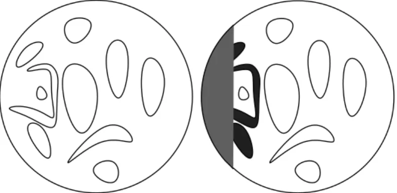
Figure 2: A coloring and the corresponding outermost loops (sketch)

1. We first derive the first of these two statements together with the uniqueness part of the second one. This will involve a detailed analysis of the CLE property, and consequences about possible ways to “explore” a CLE. Here, SLE techniques will be important.

2. We derive the existence part of the second statement using clusters of Poisson point processes of Brownian loops (the Brownian loop-soups).

In the end, we will have two remarkably different explicit constructions of these conformal loop ensembles CLEκ for each κ in (8/3, 4] (one based on SLE, one based

on loop-soups). This is useful, since many properties that seem very mysterious from one perspective are easy from the other. For example, the (expectation) fractal di-mensions of the individual loops and of the set of points not surrounded by any loop can be explicitly computed with SLE tools [40], while many monotonicity results and FKG-type correlation inequalities are immediate from the loop-soup construction [50]. One illustration of the interplay between these two approaches is already present in this paper: One can use SLE tools to determine exactly the value of the critical intensity that separates the two percolative phases of the Brownian loop-soup (and to our knowl-edge, this is the only self-similar percolation model where this critical value has been determined).

In order to try to explain the logical construction of the proof, let us outline these two parts separately in the following two subsections.

1.2

Main statements and outline: The Markovian construction

Let us now describe in more detail the results of the first part of the paper, corresponding to Sections 2 through 8. We are going to study random families Γ = (γj, j ∈ J) of

non-nested simple disjoint loops in simply connected domains. For each simply connected D, we let PD denote the law of this loop-ensemble in D. We say that this family is

conformally invariant if for any two simply connected domains D and D′ _{(that are}

not equal to the entire plane) and conformal transformation ψ : D _{→ D}′_{, the image of}

PD under ψ is PD′.

We also make the following “local finiteness” assumption: if D is equal to the unit disc U, then for any ε > 0, there are PUalmost surely only finitely many loops of radius

larger than ǫ in Γ.

Consider two simply connected domains D1 ⊂ D2, and sample a family (γj, j ∈ J)

according to the law PD2 in the larger domain D2. Then, we can subdivide the family

Γ = (γj, j ∈ J) into two parts: Those that do not stay in D1, and those that stay in D1

(we call the latter (γj, j ∈ J1)). Let us now define D∗1 to be the random set obtained

when removing from the set D1 all the loops of Γ that do not fully stay in D1, together

with their interiors. We say that the family PD satisfies restriction if, for any such D1

and D2, the conditional law of (γj, j ∈ J1) given D1∗ is PD∗

1 (or more precisely, it is the

product of PD for each connected component D of D1∗). When a family is conformally

invariant and satisfies restriction, we say that it is a Conformal Loop Ensemble (CLE). The goal of the paper is to characterize and construct all possible CLEs.

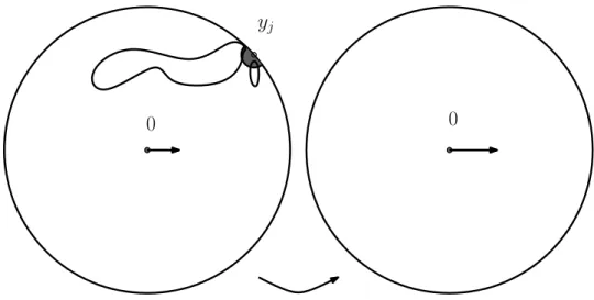
Figure 3: Restriction property (sketch): given the set of loops intersecting D2\ D1 (the

grey wedge on the left of the right figure) the conditional law of the remaining loops is an independent CLE in each component of the (interior of the) complement of this set.

By conformal invariance, it is sufficient to describe PDfor one given simply connected

domain. Let us for instance consider D to be the upper half-plane H. A first step in our analysis will be to prove that for all z ∈ H, if Γ is a CLE, then the conditional law of the unique loop γ(z) ∈ Γ that surrounds z, conditionally on the fact that γ(z) intersects the ε-neighborhood of the origin, converges as ε_{→ 0 to a probability measure} Pz _{on “pinned loops”, i.e., loops in H that touch the real line only at the origin. We}

will derive various properties of Pz_{, which will eventually enable us to relate it to SLE.}

One simple way to describe this relation is as follows:

Theorem 1.2. If Γ is a CLE, then the measure Pz _{exists for all z ∈ H, and it is}

to disconnect z from infinity in H, for some κ ∈ (8/3, 4] (we call this limit the SLEκ

bubble measure).

This shows that all the loops of a CLE are indeed in some sense “SLEκ loops” for

some κ. In fact, the way in which Pz _{will be described (and in which this theorem will}

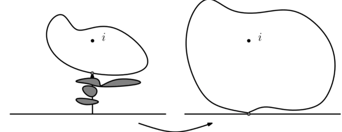
actually be proved) can be understood as follows (this will be the content of Proposition 4.1) in the case where z = i: Consider A the lowest point on [0, i]_{∩ γ(i), and H the} unbounded connected component of the domain obtained by removing from H\ [0, A] all the loops of the CLE that intersect [0, A). Consider the conformal map Φ from H onto H with Φ(i) = i and Φ(A) = 0. Then, the law of Φ(γ(i)) is exactly Pi_.

i

i

Figure 4: Description of Pi _(sketch).

Theorem 1.2 raises the question of whether two different CLE distributions can correspond to the same measure Pz_{. We will prove that it is not possible, i.e., we will}

describe a way to reconstruct the law of the CLE out of the knowledge of Pz _{only, using}

a construction based on a Poisson point process of pinned loops:

Theorem 1.3. For each κ_{∈ (8/3, 4], there exists at most one CLE such that P}z _{is the}

SLEκ bubble measure.

In a way, this reconstruction procedure can be interpreted as an “excursion theory” for CLEs. It will be very closely related to the decomposition of a Bessel process via its Poisson point process of excursions. In fact, this will enable us to relate our CLEs to the random loop ensembles defined in [43] using branching SLE processes, which we now briefly describe. Recall that when κ_{≤ 4, SLE}κ is a random simple curve from one

marked boundary point a of a simply connected domain D to another boundary point b. If we now compare the law of an SLE from a to b in D with that of an SLE from a to b′ _{in D when b6= b}′_{, then they clearly differ, and it is also immediate to check that}

the laws of their initial parts (i.e., the laws of the paths up to the first time they exit some fixed small neighborhood of a) are also not identical. We say that SLEκ is not

by Schramm and Wilson [42] (see also [43]) to be target-independent. This makes it possible to couple such processes starting at a and aiming at two different points b and b′ _{in such a way that they coincide until the first disconnection point. This in turn}

makes it possible to canonically define a conformally invariant “exploration tree” of SLE (κ, κ_{− 6) processes rooted at a, and a collection of loops called Conformal Loop} Ensembles in [43]. It is conjectured in [43] that this one-parameter collection of loops indeed corresponds to the scaling limit of a wide class of discrete lattice-based models, and that for each κ, the law of the constructed family of loops is independent of the starting point a.

The branching SLE (κ, κ−6) procedure works for any κ ∈ (8/3, 8], but the obtained loops are simple and disjoint loops only when κ ≤ 4. In this paper, we use the term CLE to refer to any collection of loops satisfying conformal invariance and restriction, while using the term CLEκ to refer to the random collections of loops constructed in

[43]. We shall prove the following:

Theorem 1.4. Every CLE is in fact a CLEκ for some κ∈ (8/3, 4].

Let us stress that we have not yet proved at this point that the CLEκ are themselves

CLEs (and this was also not established in [43]) – nor that the law of CLEκ is

root-independent. In fact, it is not proved at this point that CLEs exist at all. All of this will follow from the second part.

1.3

Main statements and outline: The loop-soup construction

We now describe the content of Sections 9 to 11. The Brownian loop-soup, as defined in [23], is a Poissonian random countable collection of Brownian loops contained within a fixed simply-connected domain D. We will actually only need to consider the outer boundaries of the Brownian loops, so we will take the perspective that a loop-soup is a random countable collection of simple loops (outer boudaries of Brownian loops can be defined as SLE8/3 loops, see [53]). Let us stress that our conformal loop ensembles

are also random collections of simple loops, but that, unlike the loops of the Brownian loop-soup, the loops in a CLE are almost surely all disjoint from one another.

The loops of the Brownian loop-soup _{L = (ℓ}j, j ∈ J) in the unit disk U are the

points of a Poisson point process with intensity cµ, where c is an intensity constant, and µ is the Brownian loop measure in U. The Brownian loop-soup measure P = Pc is

the law of this random collection _L.

When A and A′ _{are two closed bounded subsets of a bounded domain D, we denote}

by L(A, A′; D) the µ-mass of the set of loops that intersect both sets A and A′, and stay in D. When the distance between A and A′ _{is positive, this mass is finite [23].}

Similarly, for each fixed positive ǫ, the set of loops that stay in the bounded domain D and have diameter larger than ǫ, has finite mass for µ.

The conformal restriction property of the Brownian loop measure µ (which in fact characterizes the measure up to a multiplicative constant; see [53]) implies the following

two facts (which are essentially the only features of the Brownian loop-soup that we shall use in the present paper):

1. Conformal invariance: The measure Pc is invariant under any Moebius

transfor-mation of the unit disc onto itself. This invariance makes it in fact possible to define the law PD of the loop-soup in any simply connected domain D6= C as the

law of the image of_{L under any given conformal map Φ from U onto D (because} the law of this image does not depend on the actual choice of Φ).

2. Restriction: If one restricts a loop-soup in U to those loops that stay in a simply connected domain U _{⊂ U, one gets a sample of P}U.

We will work with the usual definition (i.e., the usual normalization) of the measure µ (as in [23] — note that there can be some confusion about a factor 2 in the definition, related to whether one keeps track of the orientation of the Brownian loops or not). Since we will be talking about some explicit values of c later, it is important to specify this normalization. For a direct definition of the measure µ in terms of Brownian loops, see [23].

Figure 5: Sample of a random-walk soup approximation [22] of a Brownian loop-soup in a square, by Serban Nacu

As mentioned above, [50] pointed out a way to relate Brownian loop-soups clusters to SLE-type loops: Two loops in _{L are said to be adjacent if they intersect. Denote by} C(L) the set of clusters of loops under this relation. For each element C ∈ C(L) write

C for the closure of the union of all the loops in C and denote by C the family of all C’s.

Figure 6: A loup-soup and the fillings of its outermost clusters (sketch)

We write F (C) for the filling of C, i.e., for the complement of the unbounded connected component of C_{\ C. A cluster C is called outermost if there exists no C}′

such that C ⊂ F (C′_{). The outer boundary of such an outermost cluster C is the}

boundary of F (C). Denote by Γ the set of outer boundaries of outermost clusters of_L. Let us now state the main results of this second step:

Theorem 1.5. Suppose that L is the Brownian loop-soup with intensity c in U. • If c ∈ (0, 1], then Γ is a random countable collection of disjoint simple loops that

satisfies the conformal restriction axioms.

• If c > 1, then there is almost surely only one cluster in C(L).

It therefore follows from our Markovian characterization that Γ is a CLEκ(according

to the branching SLE(κ, κ_{− 6) based definition in [43]) for some κ ∈ (8/3, 4]. We will} in fact also derive the following correspondence:

Theorem 1.6. Fix c _{∈ (0, 1] and let L be a Brownian loop-soup of intensity c on U.} Then Γ is a CLEκ where κ∈ (8/3, 4] is determined by the relation c = (3κ−8)(6−κ)/2κ.

1.4

Main statements and outline: Combining the two steps

Since every κ _{∈ (8/3, 4] is obtained for exactly one value of c ∈ (0, 1] in Theorem 1.6,} we immediately get thanks to Theorem 1.4 that the random simple loop configurations satisfying the conformal restriction axioms are precisely the CLEκ where κ ∈ (8/3, 4],

which completes the proof of Theorem 1.1 and of the fact that the following three descriptions of simple loop ensembles are equivalent:

1. The random loop ensembles traced by branching Schramm-Loewner Evolution (SLEκ) curves for κ in (8/3, 4].

2. The outer-cluster-boundary ensembles of Brownian loop-soups for c_{≤ 1.} 3. The (only) random loop ensembles satisfying the CLE axioms.

Let us now list some further consequences of these results. Recall from [1] that the Hausdorff dimension of an SLEκ curve is almost surely 1 + (κ/8). Our results therefore

imply that the boundary of a loop-soup cluster of intensity c≤ 1 has dimension 37− c −√25 + c2_{− 26c}

24 .

Note that just as for Mandelbrot’s conjecture for the dimension of Brownian boundaries [17], this statement does not involve SLE, but its proof does. In fact the result about the dimension of Brownian boundaries can be viewed as the limit when c _{→ 0 of this} one.

Furthermore we may define the carpet of the CLEκ to be the random closed set

obtained by removing from U the interiors (i.e. the bounded connected component of their complement) of all the loops γ of Γ, and recall that SLE methods allowed [40] to compute its “expectation dimension” in terms of κ. The present loop-soup construction of CLEκ enables to prove (see [29]) that this expectation dimension is indeed equal to

its almost sure Hausdorff dimension d, and that in terms of c, d(c) = 187− 7c +

√

25 + c2_{− 26c}

96 (1)

The critical loop-soup (for c = 1) corresponds therefore to a carpet of dimension 15/8. Another direct consequence of the previous results is the “additivity property” of CLE’s: If one considers two independent CLE’s in the same simply connected domain D with non-empty boundary, and looks at the union of these two, then either one can find a cluster whose boundary contains ∂D, or the outer boundaries of the obtained outermost clusters in this union form another CLE. This is simply due to the fact that each of the CLE’s can be constructed via Brownian loop soups (of some intensities c1

and c2) so that the union corresponds to a Brownian loop-soup of intensity c1 + c2.

This gives for instance a clean direct geometric meaning to the general idea (present on various occasions in the physics literature) that relates in some way two independent copies of the Ising model to the Gaussian Free Field in their large scale limit: The outermost boundaries defined by the union of two independent CLE3’s in a domain

(recall [7] that CLE3 is the scaling limit of the Ising model loops, and note that it

corresponds to c = 1/2) form a CLE4 (which corresponds to “outermost” level lines of

1.5

Further background

In order to put our results in perspective, we briefly recall some closely related work on conformally invariant structures.

Continuous conformally invariant structures giving rise to loops. There exist several natural ways to construct conformally invariant structures in a domain D. We have already mentioned the Brownian loop-soup that will turn out be instrumental in the present paper when constructing explicitely CLEs. Another natural conformally invariant structure that we have also just mentioned is the Gaussian Free Field. This is a classical basic object in Field Theory. It has been shown (see [38, 10]) that it is very closely related to SLE processes, and that one can detect all kinds of SLEs within the Gaussian Free Field. In particular, this indicates that CLEs (at least when κ = 4) can in fact also be defined and found as “geometric” lines in a Gaussian Free Field.

Discrete models. A number of discrete lattice-based models have been conjectured to give rise to conformally invariant structures in the fine-mesh limit. For some of these models, these structures can be described by random collections of loops. We have already mentioned that Smirnov [45, 46, 47] has proved this conjecture for some important models (percolation, Ising model — see also [20, 37, 38] for some other cases). Those models that will be directly relevant to the present paper (i.e., with disjoint simple loops) include the Ising model and the discrete Gaussian Free Field level lines ([47, 7, 38, 10]). The scaling limits of percolation and of the FK-model related to the Ising model give rise to interfaces that are not disjoint. These are of course also very interesting objects (see [41, 5, 48] for the description of the percolation scaling limit), but they are not the subject of the present paper. Conjecturally, each of the CLEs that we will be describing corresponds to the scaling limit of one of the so-called O(N) models, see e.g. [30, 13], which are one simple way to define discrete random collections of non-overlapping loops.

In fact, if one starts from a lattice-based model for which one controls the (con-formally invariant) scaling limit of an observable (loosely speaking, the scaling limit of the probability of some event), it seems possible (see Smirnov [46]) to use this to actually prove the convergence of the entire discrete “branching” exploration procedure to the corresponding branching SLE(κ, κ_{− 6) exploration tree. It is likely that it is} not so much harder to derive the “full” scaling limit of all interfaces than to show the convergence of one particular interface to SLE.

Another quite different family of discrete models that might (more conjecturally) be related to the CLEs that we are studying here, are the “planar maps”, where one chooses at random a planar graph, defined modulo homeomorphisms, and that are conjecturally closely related to the above (for instance via their conjectured relation with the Gaussian Free Field). It could well be that CLEs are rather directly related to random planar maps chosen in a way to contain “large holes”, such as the ones that are studied in [24]. In fact, CLEs, planar maps and the Gaussian Free Field should all be related to each other via Liouville quantum gravity, as described in [11].

Conformal Field Theory. Note finally that Conformal Field Theory, as developed in the theoretical physics community since the early eighties [2], is also a setup to describe the scaling limits of all correlation functions of these critical two-dimensional lattice models. This indicates that a description of the entire scaling limit of the lattice models in geometric SLE-type terms could be useful in order to construct such fields. CLE-based constructions of Conformal Field Theoretical objects “in the bulk” can be found in Benjamin Doyon’s papers [8, 9]. It may also be mentioned that aspects of the present paper (infinite measures on “pinned configurations”) can be interpreted naturally in terms of insertions of boundary operators.

Part one: the Markovian

characterization

2

The CLE property

2.1

Definitions

A simple loop in the complex plane will be the image of the unit circle in the plane under a continuous injective map (in other words we will identify two loops if one of them is obtained by a bijective reparametrization of the other one; note that our loops are not oriented). Note that a simple loop γ separates the plane into two connected components that we call its interior int(γ) (the bounded one) and its exterior (the unbounded one) and that each one of these two sets characterizes the loop. There are various natural distances and σ-fields that one can use for the space_{L of loops. We will} use the σ-field Σ generated by all the events of the type_{{O ⊂ int(γ)} when O spans the} set of open sets in the unit plane. Note that this σ-field is also generated by the events of the type_{{x ∈ int(γ)} where x spans a countable dense subset Q of the plane (recall} that we are considering simple loops so that O _{⊂ int(γ) as soon as O ∩ Q ⊂ int(γ)).}

In the present paper, we will consider (at most countable) collections Γ = (γj, j ∈ J)

of simple loops. One way to properly define such a collection is to identify it with the point-measure

µΓ =

X

j∈J

δγj.

Note that this space of collections of loops is naturally equipped with the σ-field gen-erated by the sets _{{Γ : #(Γ ∩ A) = k} = {Γ : µ}Γ(A) = k}, where A ∈ Σ and

k _{≥ 0.}

We will say that (γj, j ∈ J) is a simple loop configuration in the bounded simply

connected domain D if the following conditions hold: • For each j ∈ J, the loop γj is a simple loop in D.

• For each j 6= j′ _{∈ J, the loops γ}

j and γj′ are disjoint.

• For each j 6= j′ _{∈ J, γ}

j is not in the interior of γj′: The loops are not nested.

• For each ε > 0, only finitely many loops γj have a diameter greater than ε. We

call this the local finiteness condition.

All these conditions are clearly measurable with respect to the σ-field discussed above. We are going to study random simple loop configurations with some special proper-ties. More precisely, we will say that the random simple loop configuration Γ = (γj, j ∈

J) in the unit disc U is a Conformal Loop Ensemble (CLE) if it satisfies the following properties:

• Non-triviality: The probability that J 6= ∅ is positive.

• Conformal invariance: The law of Γ is invariant under any conformal transforma-tion from U onto itself. This invariance makes it in fact possible to define the law of the loop-ensemble ΓD in any simply connected domain D 6= C as the law of

the image of Γ under any given conformal map Φ from U onto D (this is because the law of this image does not depend on the actual choice of Φ). We can also define the law of a loop-ensemble in any open domain D 6= C that is the union of disjoint open simply connected sets by taking independent loop-ensembles in each of the connected components of D. We call this law PD.

• Restriction: To state this important property, we need to introduce some notation. Suppose that U is a simply connected subset of the unit disc. Define

I = I(Γ, U) =_{{j ∈ J : γ}j 6⊂ U}

and J∗ = J∗(Γ, U) = J\ I = {j ∈ J : γj ⊂ U}. Define the (random) set

U∗ = U∗(U, Γ) = U _{\ ∪}j∈Iint(γj).

This set U∗ is a (not necessarily simply connected) open subset of U (because of the local finiteness condition). The restriction property is that (for all U), the conditional law of (γj, j ∈ J∗) given U∗ (or alternatively given the family

(γj, j ∈ I)) is PU∗.

This definition is motivated by the fact that for many discrete loop-models that are conjectured to be conformally invariant in the scaling limit, the discrete analog of this restriction property holds. Examples include the O(N) models (and in particular the critical Ising model interfaces). The goal of the paper is to classify all possible CLEs, and therefore the possible conformally invariant scaling limits of such loop-models.

The non-nesting property can seem surprising since the discrete models allow nested loops. The CLE in fact describes (when the domain D is fixed) the conjectural scaling limit of the law of the “outermost loops” (those that are not surrounded by any other one). In the discrete models, one can discover them “from the outside” in such a way that the conditional law of the remaining loops given the outermost loops is just made of independent copies of the model in the interior of each of the discovered loops. Hence, the conjectural scaling limit of the full family of loops is obtained by iteratively defining CLEs inside each loop.

At first sight, the restriction property does not look that restrictive. In particular, as it involves only interaction between entire loops, it may seem weaker than the conformal exploration property of SLE (or of branching SLE(κ, κ_{− 6)), that describes the way} in which the path is progressively constructed. However (and this is the content of Theorems 1.2 and 1.3), the family of such CLEs is one-dimensional too, parameterized by κ_{∈ (8/3, 4].}

2.2

Simple properties of CLEs

We now list some simple consequences of the CLE definition. Suppose that Γ = (γj, j ∈

J) is a CLE in U.

1. Then, for any given z _{∈ U, there almost surely exists a loop γ}j in Γ such that

z _{∈ int(γ}j). Here is a short proof of this fact: Define u = u(z) to be the probability

that z is in the interior of some loop in Γ. By Moebius invariance, this quantity u does not depend on z. Furthermore, since P (J _{6= ∅) > 0, it follows that u > 0} (otherwise the expected area of the union of all interiors of loops would be zero). Hence, there exists r ∈ (0, 1) such that with a positive probability p, the origin is in the interior of some loop in Γ that intersects the slit [r, 1] (we call A this event). We now define U = U_{\ [r, 1) and apply the restriction property. If A holds, then} the origin is in the interior of some loop of Γ. If A does not hold, then the origin is in one of the connected components of ˜U and the conditional probability that it is surrounded by a loop in this domain is therefore still u. Hence, u = p + (1_{− p)u} so that u = 1.

2. The previous observation implies immediately that J is almost surely infinite. Indeed, almost surely, all the points 1− 1/n, n ≥ 1 are surrounded by a loop, and any given loop can only surround finitely many of these points (because it is at positive distance from ∂U).

3. Let M(θ) denote the set of configurations Γ = (γj, j ∈ J) such that for all j ∈ J,

the radius [0, eiθ_{] is never locally “touched without crossing” by γ}

j (in other words,

θ is a local extremum of none of the arg(γj)’s). Then, for each given θ, Γ is almost

surely in M(θ). Indeed, the argument of a given loop that does not pass through the origin can anyway at most have countably many “local maxima”, and there are also countably many loops. Hence, the set of θ’s such that Γ /_{∈ M(θ) is at} most countable. But the law of the CLE is invariant under rotations, so that P (Γ∈ M(θ)) does not depend on θ. Since its mean value (for θ ∈ [0, 2π]) is 1, it is always equal to 1.

If we now define, for all r > 0, the Moebius transformation of the unit disc such that ψ(1) = 1, ψ(_{−1) = −1 and ψ}′_{(1) = r, the invariance of the CLE law under}

ψ shows that for each given r, almost surely, no loop of the CLE locally touches ψ([_{−i, i]) without crossing it.}

4. For any r < 1, the probability that rU is entirely contained in the interior of one single loop is positive: This is because each simple loop γ that surrounds the origin can be approximated “from the outside” by a loop η on a grid of rational meshsize with as much precision as one wants. This implies in particular that one can find one such loop η in such a way that the image of one loop γ in the CLE under a conformal map from int(η) onto U that preserves the origin has an interior containing rU. Hence, if we apply the restriction property to U = int(η),

we get readily that with positive probability, the interior of some loop in the CLE contains rU. Since this property will not be directly used nor needed later in the paper, we leave the details of the proof to the reader.

5. The restriction property continues to hold if we replace the simply connected domain U _{⊂ U with the union U of countably many disjoint simply connected} domains Ui ⊂ U. That is, we still have that the conditional law of (γj, j ∈ J∗)

given U∗(or alternatively given the family (γj, j ∈ I)) is PU∗. To see this, note first

that applying the property separately for each Uigives us the marginal conditional

laws for the set of loops within each of the Ui. Then, observe that the conditional

law of the set of loops in Ui is unchanged when one further conditions on the set

of loops in _∪i′_6=iU_i′. Hence, the sets of loops in the domains U₁∗, . . . , U_i∗, . . . are in

fact independent (conditionally on (γj, j ∈ I)).

3

Explorations

3.1

Exploring CLEs – heuristics

Suppose that Γ = (γj, j ∈ J) is a CLE in the unit disc U. Suppose that ε > 0 is

given. Cut out from the disc a little given shape S = S(ε) ⊂ U of radius ε around 1. If y is a point on the unit circle, then we may write yS for y times the set S — i.e., S rotated around the circle via multiplication by y. The precise shape of S will not be so important; for concreteness, we may at this point think of S as being equal to the ε-neighborhood of 1 in the unit disc. Let U1 denote the connected component that

contains the origin of the set obtained when removing from U′

1 := U\ S all the loops

that do not stay in U1′. If the loop γ0 in the CLE that surrounds the origin did not go

out of U_{\S, then the (conditional) law of the CLE restricted to U}1 (given the knowledge

of U1) is again a CLE in this domain (this is just the CLE restriction property). We

then define the conformal map Φ1 from U1 onto U with Φ1(0) = 0 and Φ′1(0) > 0.

Now we again explore a little piece of U1: we choose some point y1 on the unit

circle and define U′

2 to be the domain obtained when removing from U1 the preimage

(under Φ1) of the shape S centered around y1 (i.e., U2′ = Φ−11 (U\ y1S)). Again, we

define the connected component U2 that contains the origin of the domain obtained

when removing from U′

2 the loops that do not stay in U2′ and the conformal map Φ2

from U2 onto U normalized at the origin.

We then explore in U2 if γ0 ⊂ U2, and so on. One can iterate this procedure until

we finally “discover” the loop γ0 that surrounds the origin. Clearly, this will happen

after finitely many steps with probability one, because at each step the derivative Φ′_n(0) is multiplied by a quantity that is bounded from below by a constant v > 1 (this is because at each step, one composes Φn with a conformal map corresponding to the

removal of at least a shape ynS in order to define Φn+1). Hence, if we never discovered

yj

0 0

Figure 7: The first exploration step (sketch)

would contradict the fact that γ0 is almost surely at positive distance from 0.

We call N the random finite step after which the loop γ0 is discovered i.e., such that

γ0 ⊂ UN but γ0 6⊂ UN +1′ . It it important to notice that at each step until N, one is in

fact repeating the same experiment (up to a conformal transformation), namely cutting out the shape S from U and then cutting out all loops that intersect S. Because of the CLE’s conformal restriction property, this procedure defines an i.i.d. sequence of steps, stopped at the geometric random variable N, which is the first step at which one discovers a loop surrounding the origin that intersects U\ yNS. This shows also that

the conditional law of the CLE in U given the fact that γ0∩ S 6= ∅ is in fact identical

to the image under y−1_N ΦN of the CLE in UN.

In the coming sections, we will use various sequences yn = yn(ε). One natural

possi-bility is to simply always choose yn = 1. This will give rise to the ε radial-explorations

that will be discussed in Section 4. However, we first need another procedure to choose yn(ε) that will enable to control the behavior of ΦN (ε), of UN (ε) and of yN (ε) as ε tends

to 0. This will then allow us show that the conditional law of the CLE in U given the fact that γ0∩ S(ε) 6= ∅ has a limit when ε → 0.

3.2

Discovering the loops that intersect a given set

The precise shape of the sets S that we will use will in fact not be really important, as long as they are close to small semi-discs. It will be convenient to define, for each y on the unit circle, the set D(y, ε) to be the image of the set {z ∈ H : |z| ≤ ε}, under the conformal map Ψ : z _{7→ y(i − z)/(i + z) from the upper half-plane H onto the unit disc} such that Ψ(i) = 0 and Ψ(0) = y. Note that _|Ψ′_{(0)| = 2, so that when ε is very small,}

the set D(y, ε) is close to the intersection of a small disc of radius 2ε around y with the unit disc. This set D(1, ε) will play the role of our set S(ε).

Suppose that Γ = (γj, j ∈ J) is a given (deterministic) simple loop-configuration in

U_{. (In this section, we will derive deterministic statements that we will apply to CLEs} in the next section.) We suppose that:

1. In Γ, one loop (that we call γ0) has 0 in its interior.

2. A⊂ U is a given closed simply connected set such that U \ A is simply connected, A is the closure of the interior of A, and the length of ∂A∩ ∂U is positive. 3. The loop γ0 does not intersect A.

4. All γj’s in Γ that intersect ∂A also intersect the interior of A.

Our goal will be to explore almost all (when ε is small) large loops of Γ that intersect A by iterating explorations of ε-discs.

When ε > 0 is given, it will be useful to have general critera that imply that a subset V of the unit disc contains D(y, ε) for at least one y ∈ U: Consider two independent Brownian motions, B1 _{and B}2 _{started from the origin, and stopped at their first hitting}

times T1 and T2 of the unit circle. Consider Ua and Ub the two connected components

of U\ (B1_{[0, T}

1]∪ B2[0, T2]) that have an arc of ∂U on their boundary. Note that for

small enough ǫ, the probability p(ε) that both Ua_{and U}b _{contain some D(y, ε) is clearly}

close to 1.

Suppose now that V is a closed subset of U such that U\ V is simply connected, and let u(V ) be the probability that one of the two random sets Ua _{or U}b _{is a subset}

of V . Then:

Lemma 3.1. For all u > 0, there exists a positive ε0 = ε0(u) such that there exists

y_{∈ ∂U with D(y, ε) ⊂ V as soon as u(V ) ≥ u.}

Proof. The definition of p(ε) and of u(V ) shows that V contains some D(y, ε) with a probability at least u− (1 − p(ε)). Since this is a deterministic fact about V , we conclude that the set V does indeed contain some set D(y, ε) for some y_{∈ ∂U as soon as} p(ε)_{≥ 1−u/2. It therefore suffices to choose ε}0in such a way that u0 = 2(1−p(ε0)).

Define now a particular class of iterative exploration procedures as follows: Let U0 = U and Φ0(z) = z. For j ≥ 0:

• Choose some yj on ∂U in such a way that Φ−1j (D(yj, ε))⊂ A.

• Define Uj+1 as the connected component that contains the origin of the set

ob-tained by removing from U′

j+1 := Uj\ Φ−1j (D(yj, ε)) all the loops in Γ that do not

stay in U′ j+1.

• Let Φj+1 be the conformal map from Uj+1 onto U such that Φj+1(0) = 0 and

There is only one way in which such an iterative definition can be brought to an end, namely if at some step N0, it is not possible anymore to find a point y on ∂U

such that Φ−1_N0(D(y, ε))_{⊂ A (otherwise it means that at some step N, one actually has} discovered the loop γ0, so that UN +1 is not well-defined but we know that this cannot

be the case because we have assumed that γ0∩ A = ∅). Such explorations (Φn, n≤ N0)

will be called ε-admissible explorations of the pair (Γ, A).

Figure 8: A domain A, sketch of a completed ε-admissible exploration of (Γ, A)

Our goal is to show that when ε gets smaller, the set UN0 is close to ˜U , where ˜U is

the connected component containing the origin of U _{\ ∪}i∈I(U)γi (here U = U\ A).

The local finiteness condition implies that the boundary of ˜U consists of points that are either on ∂U or on some loop γj (in this case, we say that this loop γj contributes

to this boundary).

Lemma 3.2. For every α > 0, there exists ε′

0 = ε′0(Γ, α, A) such that for all ε ≤ ε′0,

every loop of diameter greater than α that contributes to ∂ ˜U is discovered by any ε-admissible exploration of (Γ, A).

Proof. Suppose now that γj is a loop in Γ that contributes to the boundary of ˜U . Our

assumptions on Γ and A ensure that γj therefore intersects both the interior of A and

U_{\ A. This implies that we can define three discs d1, d2 and d3 in the interior of γj} such that d1 ⊂ U \ A, and d2 ⊂ d3 ⊂ A.

Suppose that for some n _{≤ N}0, this loop γj has not yet been discovered at step n.

Since γj ∩ ∂ ˜U 6= ∅ and ˜U ⊂ Un, we see that γj ⊂ Un. Since this loop has a positive

diameter, and since Γ is locally finite, we can conclude that with a positive probability u that depends on (Γ, A, γj, d1, d2, d3), two Brownian motions B1 and B2 started from

The set_A γj 0 B1 B2 d1

Figure 9: The loop γj, the three discs and the Brownian motions (sketch)

• They both enter d1 without hitting A or ∂U or any of the other loops γi for

i_{∈ I(U).}

• They both subsequently enter d2 without going out of int(γj).

• They both subsequently disconnect d2 from the boundary of d3 before hitting it.

(This in particular guarantees that the curves hit one another within the annulus d3\ d2.)

• They both subsequently hit ∂U without going out of A.

This shows that one of the sets Ua _{and U}b _{as defined before Lemma 3.1 is contained in}

A with probability at least u. In fact, if we stop the two Brownian motions at their first exit of Uninstead on the hitting time of ∂U, the same phenomenon will hold: One of the

two sets Ua

n and Unb (with obvious notation) will be contained in Un∩A with probability

at least u. By conformal invariance of planar Brownian motion, if we apply Lemma 3.1 to the conformal images of these two Brownian motions under Φn, we get that if ε is

chosen to be sufficiently small, then it is always possible to find an ε-admissible point yn+1. Hence, N0 > n, i.e. n is not the final step of the exploration.

As a consequence, we see that the loop γj is certainly discovered before N0, i.e., that

γj ⊂ U \ UN0, for all ε ≤ ε′0(γj, Γ, A). The lemma follows because for each positive α,

there are only finitely many loops of diameter greater than α in Γ.

Loosely speaking, this lemma tells us that indeed, UN0 converges to ˜U as ε → 0.

where ˜Φ denotes the conformal map from ˜U onto U with ˜Φ(0) = 0 and ˜Φ′_{(0) > 0. Let}

us first note that ˜U _{⊂ U}N0 because the construction of UN0 implies that before N0 one

can only discover loops that intersect A.

Let us now consider a two-dimensional Brownian motion B started from the origin, and define T (respectively ˜T ) the first time at which it exits U (resp. ˜U). Let us make a fifth assumption on A and Γ:

• 5. Almost surely, BT ∈ ∂U ∪ (∪jint(γj)).

Note that this is indeed almost surely the case for a CLE (because Γ is then inde-pendent of BT so that BT is a.s. in the interior of some loop if it is not on ∂U). This

assumption implies that almost surely, either ˜T < T (and B_T˜ is on the boundary of

some loop of positive diameter) or BT = B_T˜ ∈ ∂U. The previous result shows that if ˆT

denotes the exit time of UN0 (for some given ε-admissible exploration), then ˆT = ˜T for

all small enough ε.

It therefore follows that ΦN0 converges to ˜Φ in the sense that for all proper compact

subsets K of U, the functions Φ−1_N0 converge uniformly to ˜Φ−1 _{in K as ε→ 0. We shall}

use this notion of convergence on various occasions throughout the paper. Note that this it corresponds to the convergence with respect to a distance d, for instance

d(ϕ1, ϕ2) = X n≥1 2−n max |z|≤1−1/nkϕ −1 1 (z)− ϕ−12 (z)k.

We have therefore shown that:

Lemma 3.3. For each given loop configuration and A (satisfying conditions 1-5), d(ΦN0, ˜Φ) tends to 0 as ε → 0, uniformly with respect to all ε-admissible explorations

of (Γ, A).

Suppose now that γ0 intersects the interior of A. Exactly the same arguments show

that there exists ε1 = ε(Γ, A) such that for all “ε-admissible choices” of the yj’s for

ε_{≤ ε}1, one discovers γ0 during the exploration (and this exploration is then stopped in

this way).

3.3

Discovering random configurations along some given line

For each small δ, we define the wedge Wδ ={ueiθ : u ∈ (0, 1) and |θ| ≤ δ}. For each

positive r, let ˜Wr denote the image of the positive half disc{z ∈ U : Re (z) > 0} under

the Moebius transformation of the unit disc with ψ(1) = 1, ψ(_{−1) = −1 and ψ}′_{(1) = r.}

Note that r 7→ ˜Wr is continuously increasing on (0, 1] from ˜W0+ = {1} to the positive

half-disc ˜W1. For all non-negative integer k≤ 1/δ, we then define

Suppose that δ is fixed, and that Γ is a loop-configuration satisfying conditions 1-5 for all set Aδ,k _{for k ≤ K, where}

K = K(Γ, δ) = max{k : γ0∩ Aδk =∅}.

We are going to define the conformal maps ˜Φδ,1_{, . . . , ˜Φ}δ,K_{corresponding to the conformal}

map ˜Φ when A is respectively equal to Aδ,1_{, . . . , A}δ,K_.

For each given δ and ε, it is possible to define an ε-admissible chain of explorations of Γ and Aδ,1_{, A}δ,2_{, . . . as follows: Let us first start with an ε-admissible exploration}

of (Γ, Aδ,1_{). If K ≥ 1, then such an exploration does not encounter γ}

0, and we then

continue to explore until we get an ε-admissible exploration of (Γ, Aδ,2_{), and so on, until}

the last value K′ _{of k for which the exploration of (Γ, A}δ,k_{) fails to discovers γ}

0. In this

way, we define conformal maps

˜

Φδ,1_ε , . . . , ˜Φδ,K_ε ′

corresponding to the sets discovered at each of these K′_{explorations. Note that K}′ _{≥ K.}

One can then also start to explore the set Aδ,K′₊₁

until one actually discovers the loop γ0.

Figure 10: An exploration-chain and γ0 (sketch)

This procedure therefore defines a single ε-admissible exploration (via some sequence (Φn, yn)), that explores the sets Aδ,j’s in an ordered way, and finally stops at some step

N, i.e., the last step before one actually discovers γ0. We call this an ε-admissible

exploration chain of Aδ,1_{, A}δ,2_{, . . .. Our previous results show that uniformly over all}

such ε-admissible exploration-chains (for each given Γ and δ): • K′ _{= K for all sufficiently small ε.}

• limε→0( ˜Φδ,1ε , . . . , ˜Φδ,K ′

ε ) = ( ˜Φδ,1, . . . , ˜Φδ,K).

We now suppose that Γ is a random loop-configuration. Then, for each δ, K = K(Γ, δ) is random. We assume that for each given δ, the conditions 1-5 hold almost surely for each of the K sets Aδ

1, . . . , AδK. The previous results therefore hold almost

surely; this implies for instance that for each η > 0, there exists ε2(δ) such that for all

such ε-admissible exploration-chain of (Γ, Aδ

1, Aδ2, . . .) with ε ≤ ε2(δ),

P (K′ = K and d( ˜Φδ,K_ε , ˜Φδ,K) < η)≥ 1 − η.

We will now wish to let δ go to 0 (simultaneously with ε, taking ε(δ) sufficiently small) so that we will (up to small errors that disappear as ε and δ vanish) just explore the loops that intersect the segment [0, 1] “from 1 to 0” up to the first point at which it meets γ0. We therefore define

R = max{r ∈ [0, 1] , r ∈ γ0}.

We define the open set ˆU as the connected component containing the origin of the set obtained by removing from U_{\ [R, 1] all the loops that intersect (R, 1]. Note that} γ0 ⊂ ˆU ∪ {R}. We let ˆΦ denote the conformal map from ˆU onto U such that ˆΦ(0) = 0

and ˆΦ′_{(0) > 0. We also define ˆy = ˆΦ(R).}

γ

1

R

ˆ

U

Figure 11: Exploring up to γ0 (sketch)

Proposition 3.4. For a well-chosen function ε3 = ε3(δ) (that depends on the law

of Γ only), for any choice of ε(δ)-admissible exploration-chain of the random loop-configuration Γ and Aδ,1_{, . . . with ε(δ) ≤ ε}

3(δ), the random pair (ΦN, yN) converges

Proof. Note first that our assumptions on Γ imply that almost surely Φδ,K _{→ ˆΦ as}

δ _{→ 0 (this is a statement about Γ that does not involve explorations).}

We know that γ0 intersects Aδ,K+1 \ Aδ,K. The local finiteness of Γ and the fact

that any two loops are disjoint therefore implies that the diameter of the second largest loop (after γ0) of Γ that intersects this set almost surely tends to 0 as δ → 0. This in

particular implies that almost surely, the distance between ΦN and ˜Φδ,Kε tends to 0 as

δ→ 0 (uniformly with respect to the choice of the exploration, as long as ε(δ) tends to 0 sufficiently fast).

Recall finally that for each given δ, ˜Φδ,K

ε → Φδ,K as ε→ 0. Hence, if ε(δ) is chosen

small enough, the map ΦN indeed converges almost surely to ˆΦ as δ→ 0.

It now remains to show that yN → ˆy. Note that R ∈ UN (because at that step, γ0

has not yet been discovered), that R _{∈ A}δ,K′₊₁

\ Aδ,K′

(with high probability, if ε(δ) is chosen to be small enough). On the other hand, the definition of the exploration procedure and of K′ shows that

Φ−1_N (D(yN, ε))∩ (Aδ,K

′₊₁

\ Aδ,K′

)6= ∅

so that if we choose ε(δ) small enough, then the Euclidean distance between Φ−1_N (D(yN, ε))

and R tends to 0 almost surely.

Let us look at the situation at step N: The loop ΦN(γ0) in the unit disc is intersecting

D(yN, ε) (by definition of N), and it contains also the point ΦN(R) (because R ∈ γ0).

Suppose that |ΦN(R) − yN| does not almost surely tend to 0 (when δ → 0); then,

with positive probability, we could find a sequence δj → 0 such that ΦN(R) and yN

converge to different points on the unit circle along this subsequence. In particular, the harmonic measure at the origin of any of the two parts of the loop between the moment it visits ΦN(R) and the ε-neighborhood of yN in U is bounded away from 0. Hence,

this is also true for the preimage γ0 under ΦN: γ0 contains two disjoint paths from R

to Φ−1_N (D(yN, ε)) such that their harmonic measure at 0 in U is bounded away from 0.

Recall that Φ−1_N (D(yN, ε))⊂ Aδ,K

′₊₁

. In the limit when δ_{→ 0, we therefore end up with} a contradiction, as we have two parts of γ0 with positive harmonic measure from the

origin, that join R to some point of [R, 1], which is not possible because γ0∩ (R, 1] 6= ∅

and γ0 is a simple loop. Hence, we can conclude that |ΦN(R)− yN| → 0 almost surely.

Finally, let us observe that ΦN(R) → ˆΦ(R) almost surely (this follows for instance

from the fact that a continuous path that stays inside γ0 and joins the origin to R stays

both in all UN’s and in ˆU). It follows that yN converges almost surely to ˆy.

4

The one-point pinned loop measure

4.1

The pinned loop surrounding the origin in U

We will use the previous exploration mechanisms in the context of CLEs. It is natural to define the notion of Markovian explorations of a CLE. Suppose now that Γ is a CLE in the unit disc and that ε is fixed. When γ0 ∩ D(1, ε) = ∅, define just as before the

set U1 and the conformal map Φ1 obtained by discovering the set of loops Γ1 of Γ that

intersect D(y0, ε). Then we choose y1 and proceed as before, until we discover (at step

N + 1) the loop γ0 that surrounds the origin. We say that the exploration is Markovian

if for each n, the choice of yn is measurable with respect to the σ-field generated by

Γ1, . . . , Γn, i.e., the set of all already discovered loops.

A straightforward consequence of the CLE’s restriction property is that for each n, conditionally on Γ1, y1, . . . , Γn, yn(and n≤ N), the law of the set of loops of Γ that stay

in Un is that of a CLE in Un. In other words, the image of this set of loops under Φn is

independent of Γ1, y1, . . . , Γn, yn (on the event {n ≤ N}). In fact, we could have used

this independence property as a definition of Markovian explorations (it would allow extra randomness in the choice of the sequence yn).

In other words, an exploration is Markovian if we can choose ynas we wish using the

information about the loops that have already been discovered, but we are not allowed to use any information about the yet-to-be-discovered loops. This ensures that one obtains an iteration of i.i.d. explorations as argued in subsection 3.1. In particular, if an exploration is Markovian, the random variable N is geometric

P (N _{≥ n) = P (γ}0∩ D(1, ε) = ∅)n,

and y_N−1Φ−1_N (γ0) is distributed according to the conditional law of γ0 given{γ ∩D(1, ε) 6=

∅}.

Recall that a CLE is a random loop configuration such that for any given δ and k _{≤ 1/δ, almost surely, all loops that intersect A}δ,k _{also intersect its interior. We can}

therefore apply Proposition 3.4, and use Markovian ε(δ)-admissible successive explo-rations of Aδ,1_{, A}δ,2_{, . . . Combining this with our description of the conditional law of γ}

0

given _{{γ ∩ D(1, ε) 6= ∅}, we get the following result:}

Proposition 4.1. When ε→ 0, the law of γ0conditioned on the event{γ0∩D(1, ε) 6= ∅}

converges to the law of ˆy−1_Φ(γˆ _{0) (using for instance the weak convergence with respect} to the Hausdorff topology on compact sets).

Note that local finiteness of the CLE ensures that ˆΦ(γ0) is a simple loop in U that

intersects ∂U only at ˆy, so that ˆy−1_Φ(γˆ _{0) is indeed a loop in U that touches ∂U only at} 1.

This limiting law will inherit from the CLE various interesting properties. The loop γ0in the CLE can be discovered along the ray [1, 0] in the unit disc as in this proposition,

but one could also have chosen any other smooth continuous simple curve from ∂U to 0 instead of that ray and discovered it that way. This fact should correspond to some property of the law of this pinned loop. Conformal invariance of the CLE will also imply some conformal invariance properties of this pinned loop. The goal of the coming sections is to derive and exploit some of these features.

Figure 12: The law of γ0 conditioned on the event{γ0∩ D(1, ε) 6= ∅} converges (sketch)

4.2

The infinite measure on pinned loops in H

We are now going to associate to each CLE a natural measure on loops that can loosely be described as the law of a loop “conditioned to touch a given boundary point”. In the previous subsection, we have constructed a probability measure on loops in the unit disc that was roughly the law of γ0 (the loop in the CLE that surrounds the origin)

“conditioned to touch the boundary point 1”. We will extend this to an infinite measure on loops that touch the boundary at one point; the measure will be infinite because we will not prescribe the “size” of the boundary-touching loop; it can be viewed as a CLE “excursion measure” (“bubble measure” would also be a possible description). We find it more convenient at this stage to work in the upper half-plane rather than

Figure 13: The construction of µi _(sketch)

the unit disc because scaling arguments will be easier to describe in this setting. We therefore first define the probability measure µi _{as the image of the law of ˆΦ(γ}

0) under

the conformal map from U onto the half-plane that maps 0 to i, and ˆy to 0 (we use the notation µi _{instead of P}i _{as in the introduction, because we will very soon be handling}

measures that are not probability measures). In other words, the probability measure µi _{is the limit as ε → 0 of the law of the loop γ(i) that surrounds i in a CLE in the}

upper half-plane, conditioned by the fact that it intersects the set Cε defined by

Cε={z ∈ H : |z| = ε}.

For a loop-configuration Γ in the upper half-plane and z _{∈ H, we denote by γ(z)} the loop of Γ that surrounds z (if this loop exists).

When z = iλ for λ > 0, scale invariance of the CLE shows that the limit as ε _{→ 0} of the conditional law of γ(iλ) given that it intersects the disc of radius λε exists, and that it is just the image of µi _{under scaling.}

Let us denote by u(ε) the probability that the loop γ(i) intersects the disc of radius ε around the origin in a CLE. The description of the measure µi _{(in terms of ˆΦ) derived}

in the previous section shows that at least for almost all λ sufficiently close to one, the loop that surrounds i also surrounds iλ and i/λ with probability at least 1/2 under µi_,

and that i/λ as well as λi are a.s. not on γ(i) (when λ is fixed). Let Oi denote the interior of the loop γ(i). We know that

lim

ε→0

P (λi_{∈ O}i and γ(i)∩ Cλε 6= ∅)

u(λε) = µ

i_(λi

∈ Oi).

On the other hand, the scaling property of the CLE shows that when ε→ 0, P (λi_{∈ O}i and γ(i)∩ Cλε 6= ∅)

u(λε)

= P (i∈ Oλi and γ(λi)∩ Cλε6= ∅) u(λε)

= P (i/λ∈ Oi and γ(i)∩ Cε6= ∅)

u(ε) × u(ε) u(λε) ∼ µi(i/λ_{∈ O}i)× u(ε) u(λε)

Hence, for all λ sufficiently close to 1, we conclude that lim ε→0 u(λε) u(ε) = µi_{(i/λ∈ O} i) µi_{(λi∈ O} i) .

If we call f (λ) this last quantity, this identity clearly implies that this convergence in fact holds for all positive λ, and that f (λλ′) = f (λ)f (λ′). Furthermore, we see that f (λ)_{→ 1 as λ → 1. Hence:}

Proposition 4.2. There exists a β _{≥ 0 (β cannot be negative since ε 7→ u(ε) is} non-decreasing) such that for all positive λ,

f (λ) = lim

ε→0

u(λε) u(ε) = λ

This has the following consequence: Corollary 4.3. u(ε) = εβ+o(1) _{as ε→ 0+.}

Proof. Note that for any β′ _{< β < β}′′_{, there exists ε}

0 = 2−n0 such that for all ε≤ ε0,

2β′ < u(2ε)/u(ε) < 2β′′. Hence, for all n_{≥ 0 it follows that}

u(ε0)2−nβ ′′

< u(ε02−n) < u(ε0)2−nβ ′

.

It follows that u(ε02−n) = 2−nβ+o(n) when n→ ∞. Since ε 7→ u(ε) is an non-decreasing

function of ε, the corollary follows.

Because of scaling, we can now define for all z = iλ, a measure µz _{on loops γ(z)}

that surround z and touch the real line at the origin as follows: µz(γ(z)∈ A) = λ−βµi(λγ(i)∈ A)

for any measurable set_{A of loops. This is also the limit of u(ε)}−1 _{times the law of γ(z)}

in an CLE, restricted to the event {γ(z) ∩ Cε6= ∅}.

Let us now choose any z in the upper half-plane. Let ψ = ψznow denote the Moebius

transformation from the upper half-plane onto itself with ψ(z) = i and ψ(0) = 0. Let λ = 1/ψ′(0). Clearly, for any given a > 1, for any small enough ε, the image of Cε

under ψ is “squeezed” between the circles Cε/aλ and Caε/λ. It follows readily (using the

fact that f (a)_{→ 1 as a → 1) that the measure µ}z _{defined for all measurable A by}

µz(γ(z)∈ A) = λ−β_µi_(ψ−1_{(γ(i))∈ A)}

can again be viewed as the limit when ε _{→ 0 of u(ε)}−1 _{times the distribution of γ(z)}

restricted to _{{γ(z) ∩ C}ε6= ∅}.

Finally, we can now define our measure µ on pinned loops. It is the measure on simple loops that touch the real line at the origin and otherwise stay in the upper half-plane (this is what we call a pinned loop) such that for all z ∈ H, it coincides with µz _{on the set of loops that surround z. Indeed, the previous limiting procedure shows}

immediately that for any two points z and z′_{, the two measures µ}z _{and µ}z′

coincide on the set of loops that surround both z and z′_{. On the other hand, we know that a}

pinned loop necessarily surrounds a small disc: thus, the requirement that µ coincides with the µz_{’s (as described above) fully determines µ.}

Let us sum up the properties of the pinned measure µ that we will use in what follows:

• For any conformal transformation ψ from the upper half-plane onto itself with ψ(0) = 0, we have

ψ_{◦ µ = |ψ}′(0)_|−βµ.

This is the conformal covariance property of µ. Note that the maps z 7→ −za/(z − a) for real a _{6= 0 satisfy ψ}′_{(0) = 1 so that µ is invariant under these}

transforma-tions.

• For each z in the upper half-plane, the mass µ({γ : z ∈ int(γ)}) is finite and equal to ψ′₍₀₎β_{, where ψ is the conformal map from H onto itself with ψ(0) = 0 and}

ψ(z) = i.

• For each z in the upper half-plane, the measure µ restricted to the set of loops that surround z is the limit as ε _{→ 0+ of u(ε)}−1 _{times the law of γ(z) in a}

CLE restricted to the event {γ(z) ∩ Cε 6= ∅}. In other words, for any bounded

continuous (with respect to the Hausdorff topology, say) function F on the set of loops,

µ(1_{{z is surrounded byγ}}F (γ)) = lim

ε→0

1

u(ε)E(1{γ(z)∩Cε6=∅}F (γ(z))).

Since this pinned measure is defined in a domain with one marked point, it is also quite natural to consider it in the upper half-plane H, but to take the marked point at infinity. In other words, one takes the image of µ under the mapping z _{7→ −1/z from H} onto itself. This is then a measure µ′ _{on loops “pinned at infinity, i.e. on double-ended}

infinite simple curves in the upper-half plane that go from and to infinity. It clearly also has the scaling property with exponent β, and the invariance under the conformal maps that preserve infinity and the derivative at infinity is just the invariance under horizontal translations.

4.3

Discrete radial/chordal explorations, heuristics, background

We will now (and also later in the paper) use the exploration mechanism corresponding to the case where all points yn are chosen to be equal to 1, instead of being tailored in

order for the exploration to stay in some a priori chosen set A as in Section 3. Let us describe this discrete radial exploration (this is how we shall refer to it) in the setting of the upper half-plane H: We fix ε > 0, and we wish to explore the CLE in the upper half-plane by repeatedly cutting out origin-centered semi-circles Cǫ of radius ε (and the

loops they intersect) and applying conformal maps. The first step is to consider the set of loops that intersect Cε. Either we have discovered the loop γ(i) (i.e., the loop

that surrounds i), in which case we stop, or we haven’t, in which case we define the connected component of the complement of these loops in H\ Cε that contains i, and

map it back onto the upper half-plane by the conformal map ϕε

1 such that ϕε1(i) = i

and (ϕε