HAL Id: hal-01794678
https://hal.archives-ouvertes.fr/hal-01794678
Submitted on 17 May 2018HAL is a multi-disciplinary open access archive for the deposit and dissemination of sci-entific research documents, whether they are pub-lished or not. The documents may come from teaching and research institutions in France or abroad, or from public or private research centers.
L’archive ouverte pluridisciplinaire HAL, est destinée au dépôt et à la diffusion de documents scientifiques de niveau recherche, publiés ou non, émanant des établissements d’enseignement et de recherche français ou étrangers, des laboratoires publics ou privés.
Heat Flux estimation in WEST divertor with embedded
thermocouples
J. Gaspar, Y. Corre, M. Firdaouss, J.-L. Gardarein, D. Guilhem, M. Houry, C.
Le Niliot, M. Missirlian, C. Pocheau, Fabrice Rigollet
To cite this version:
J. Gaspar, Y. Corre, M. Firdaouss, J.-L. Gardarein, D. Guilhem, et al.. Heat Flux estimation in WEST divertor with embedded thermocouples. 7th European Thermal-Sciences Conference, Jun 2016, Krakow, Poland. pp.292 - 303, �10.1088/1742-6596/745/3/032091�. �hal-01794678�
Journal of Physics: Conference Series
PAPER • OPEN ACCESS
Heat Flux estimation in WEST divertor with
embedded thermocouples
To cite this article: J. Gaspar et al 2016 J. Phys.: Conf. Ser. 745 032091
View the article online for updates and enhancements.
Related content
THE DIMENSIONS OF THERMOCOUPLE RECEIVERS
Edison Pettit
-THERMOCOUPLE OBSERVATIONS ON THE TOTAL RADIATION FROM VARIABLE STARS OF LONG PERIOD
E. Pettit and S. B. Nicholson
-Mathematical simulation of thermocouple characteristics
A A Abouellail, M A Kostina, S I Bortalevich et al.
Heat Flux estimation in WEST divertor with embedded
thermocouples
J. Gaspar1, Y. Corre2, M. Firdaouss2, J-L. Gardarein1, D. Guilhem2, M. Houry2,
C. Le Niliot1, M. Missirlian2, C. Pocheau2, F. Rigollet1
1 IUSTI UMR 7343 CNRS, Aix-Marseille University - 5 rue Enrico Fermi - 13453 Marseille - France
2 CEA, IRFM, Cadarache 13108 Saint Paul lez Durance, France Jonathan.gaspar@univ-amu.fr
Abstract. The present paper deals with the surface heat flux estimation with embedded
thermocouples (TC) in a Plasma Facing Component (PFC) of the WEST Tokamak. A 2D nonlinear unsteady calculation combined with the Conjugate Gradient Method (CGM) and the adjoint state is achieved in order to estimate the time evolution of the heat flux amplitude and decay length 𝜆𝑞. The method is applied on different synthetic measurements in order to evaluate
the accuracy of the method. The synthetic measurements are generated with realistic values of 𝜆𝑞 and magnitudes as those expected for ITER.
1. Introduction
Understanding heat flux deposition processes on Plasma Facing Components (PFC) is essential for PFC designs in order to allow reliable high power steady state plasma operations. In ITER, the PFCs will experience extreme heat and particle loads in steady state. WEST (W for tungsten Environment in Steady-state Tokamak) provides an integrated platform for testing the ITER divertor components under combined heat and particle loads in a tokamak environment [1]. One of the main objectives of the WEST project is to study the behavior of ITER-like actively cooled tungsten (W) Plasma Facing Units (PFU), in order to mitigate the risks for ITER [2]. The PFU should withstand heat fluxes close to the heat fluxes during ITER operations, which are expected to be around 10 MW.m-2 in steady state. It is therefore necessary to be able to measure these high heat fluxes in order to know their true amplitude and spatial distribution on the PFC surface. To achieve these objectives several thermal diagnostics (IR camera, calorimetry, embedded fibers Bragg grating and thermocouples) are planned for WEST and especially in the lower divertor where the ITER-like components will be integrated.
In the first part of the paper, the WEST lower divertor and the PFCs with embedded thermocouples (TC) are described (section 2). Then, the conjugate gradient method associated with a spatial a priori knowledge on the heat flux is presented for the estimation of the time evolution and the decay length 𝜆𝑞 of the heat flux (section 3). The results and the accuracy of the method with synthetics data are discussed based on 2D (section 4) and 3D modelling (section 5).
2. WEST lower divertor
The main interaction between plasma and wall takes place in the divertor. The WEST lower divertor target is located at the bottom of the chamber (figure 1a). Its role is to sustain the power conducted through the X-point to the strike points. The WEST divertor consists of 12 independent toroidal sectors of 30° (one sector is represented in the figure 1b), each composed of 38 PFUs for a total of 456 to form a toroidal ring structure. The complete building of the actively cooled divertor, with W monoblocks, will take several years, longer than the other changes required. As a consequence, it has been decided to begin the operations sooner, by using a mix of actively cooled PFCs (bulk W) in combination with actively cooled W coated graphite PFCs (W-coating are 15m thick) [3]. The operation with non-7th European Thermal-Sciences Conference (Eurotherm2016) IOP Publishing Journal of Physics: Conference Series 745 (2016) 032091 doi:10.1088/1742-6596/745/3/032091
Content from this work may be used under the terms of theCreative Commons Attribution 3.0 licence. Any further distribution
of this work must maintain attribution to the author(s) and the title of the work, journal citation and DOI.
actively cooled PFCs is a good opportunity to monitor the temperature with embedded measurements. The PFU is divided into two Plasma Facing Components (PFCs), one in a Low Field Side (LFS) called the outer PFC and one in the High Field Side (HFS) called the inner PFC. Then it will be progressively replaced by the ITER-like W PFU, made of W monoblocks bonded to a copper alloy tube [4]. At the start, one sector will be a mix of actively cooled ITER-like W PFU and inertial graphite components with W coating (full inertial components in the 11 other sectors).
A total of 20 TCs is embedded in the inertial graphite PFCs (red point in the figure 1b) in order to study the heat load pattern on the divertor in the toroidal (ripple effect due to 18 superconducting toroidal field coils with periodic heat flux every 20°) and poloidal (heat flux decay length due to the Scrape Off Layer (SOL) physic) directions. Here we present the use of the 4 TCs embedded in the outer PFC at the maximal heat flux location in the toroidal direction [3]. The 4 TCs will be named TC Inboard (TCI), TC Middle Inboard (TCMI), TC Middle Outboard (TCMO), TC Outboard (TCO) and they are respectively at the poloidal coordinate 31, 68.5, 106 and 143.5mm (x=0 is the left side of the PFC).
The divertor X-point configuration allows access to a wide range of plasma equilibrium. In this paper we will focus on a particular configuration called Far X-Point (FXP), with X-point localized around 7cm above the divertor (figure 1a). In this configuration the heat flux profile along the poloidal direction is very peaked at the strike point locations (intersections of red line and lower divertor in the figure 1a). The main parameter of the peaked distribution of the heat flux is the value of 𝜆𝑞, the characteristic decay length of the heat flux density in the SOL which is expected to vary between 2.5 and 10mm.
a) b)
c)
Figure 1. a) Poloidal magnetic field configuration (Far X-Point) in the WEST Tokamak. b) Lower divertor view. c) 2D sketch of the PFC with 4TCs (the surface exposed to the plasma is on the top). 3. Heat flux estimation by the Conjugate Gradient Method with adjoint state
3.1. Direct problem
In the paper, x represents the poloidal direction, y the toroidal direction and z the depth in the PFC. Figure 1c shows the geometry and the dimensions. The PFC is made of graphite coated on top and side with a thin tungsten deposit (< 30 µm). Due to the thin layer of the coating in regard to the time step (50ms) of the study, it will be taken into account only by the change of the emissivity at the surface. The dependency of the thermal properties of graphite with temperature is taken into account. The tiles are mounted onto the support plate by the round holes at the bottom of the PFC. Moreover, the WEST 7th European Thermal-Sciences Conference (Eurotherm2016) IOP Publishing Journal of Physics: Conference Series 745 (2016) 032091 doi:10.1088/1742-6596/745/3/032091
chamber is under high vacuum condition during operation (no convection exchanges). The PFC exchanges a radiative heat flux with the surrounding surfaces that are assumed to behave like the blackbody at Trad=T0, the emissivity of the graphite and the W coating is assumed known (respectively 𝜀𝐺= 0.8 and 𝜀𝑊= 0.3). The domain is initially at the same temperature, then the boundary surface Г1 is
subjected to a heat flux 𝜙(𝑥, 𝑦, 𝑡). Furthermore for a single PFC the heat flux is quite uniform in the toroidal direction (variation under 10%). This leads us to assume the heat transfer problem as a bi-dimensional problem (in x and z). This simplification allows us to save computing time and the accuracy of 2D versus 3D calculations will be studied in this paper. The mathematical formulation of this transient heat conduction problem is given as follows (for clarity we note 𝑇 = 𝑇(𝑥, 𝑧, 𝑡)):
𝜌𝐶𝑝(𝑇)𝜕𝑇𝜕𝑡− ∇⃗⃗ . (𝜆(𝑇)∇⃗⃗ (𝑇)) = 0 in Ω (1a) −𝜆(𝑇) 𝜕𝑇 𝜕𝑛2= 𝜀𝑊𝜎(𝑇 4− 𝑇 𝑟𝑎𝑑4) on Г2 (1d) −𝜆(𝑇) 𝜕𝑇 𝜕𝑛1= 𝜀𝑊𝜎(𝑇4− 𝑇𝑟𝑎𝑑 4) − 𝜙(𝑥, 𝑡) on Г 1 (1b) −𝜆(𝑇) 𝜕𝑇 𝜕𝑛3= 𝜀𝐺𝜎(𝑇4− 𝑇𝑟𝑎𝑑 4) on Г3 (1e) 𝑇 = 𝑇0 in Ω at t = 0 (1c)
This mathematical formulation (as the adjoint and sensitivity problem) is solved by the finite element method with the software CAST3M.
3.2. Inverse problem
We denote 𝑝, the function to be determined, in our case this function is the heat flux 𝜙(𝑥, 𝑡):
𝑝(𝑥, 𝑡) = 𝜙(𝑥, 𝑡) (2)
Four internal temperatures are measured by type N thermocouples (figure 1), embedded at 7.5mm from the surface, with acquisition time step of 50ms. The objective of the inverse analysis is to determine the heat flux given the unsteady embedded measurement at the TC locations. We note Y(x,z,t) the temperature data taken over time by the four TCs in the PFC. The inverse heat conduction problem consists in the determination of p(x,t) minimizing T(x,z,t) - Y(x,z,t). For this, we define the cost function which is the following quadratic criterion:
𝐽(𝑝) =1 2∫ ∑ ( 4 𝑖=1 𝑡𝑓 0 𝑇(𝑥𝑖, 𝑧𝑖 = 7.5𝑚𝑚, 𝑡) − 𝑌(𝑥𝑖, 𝑧𝑖 = 7.5𝑚𝑚, 𝑡))² dt (3)
The Conjugate Gradient Method (CGM) is the iterative process used to estimate the function 𝐩 by minimizing the cost function 𝐽(𝐩). The CGM calculates the new iterate 𝐩𝑛+1 from the previous iteration
𝐩𝑛 (with 𝑛 the iteration number), by:
𝐩𝑛+1= 𝐩𝑛− 𝛾𝑛𝐝𝑛 (4)
where 𝛾𝑛 is the step size, determined by the resolution of the sensitivity problem, and 𝐝𝑛 is the direction
of descent given by:
𝐝𝑛= ∇𝐽(𝐩𝑛) + 𝛃𝑛𝐝𝑛−1 with 𝐝0= ∇𝐽(𝐩0) (5)
where ∇𝐽(𝐩𝑛) is the gradient of the cost function, determined by the resolution of the adjoint problem
and the conjugation coefficient 𝛃𝑛 is computed with the Polak-Ribière-Polyak’s version of the CGM.
The sensitivity and adjoint problem will not be developed in this paper, the reader can refer to previous work to see the details [5].
3.3. Heat flux profile
In our case with only four TCs, we need a priori information on the unknowns to solve the inverse problem. Eich et al. showed for the JET and ASDEX divertors [6] that the spatial distribution of the heat flux in the outer side can be expressed by a heuristic formulation, built with IR thermography during Carbon-wall operations, defined by:
𝑝(𝑥, 𝑡) = 𝜙(𝑥, 𝑡) = 𝜙𝑀(𝑡)𝑒𝑥𝑝 [(𝐶2)2−𝑥−𝑥0 𝜆𝑞𝑓𝑥] 𝑒𝑟𝑓𝑐 ( 𝐶 2− 𝑥−𝑥0 𝐶𝜆𝑞𝑓𝑥) with 𝜙(𝑥 > 143𝑚𝑚, 𝑡) = 0 (6)
7th European Thermal-Sciences Conference (Eurotherm2016) IOP Publishing Journal of Physics: Conference Series 745 (2016) 032091 doi:10.1088/1742-6596/745/3/032091
where 𝑥 is the target coordinate, 𝑥0 is the strike point location, 𝜆𝑞 is the power decay length inside the scrape off layer, 𝑓𝑥 is the magnetic flux expansion at the PFC target and 𝐶 is a constant. For the FXP configuration studied here 𝑓𝑥=3 and 𝐶=0.4. The heat flux is set equal to 0 for 𝑥 > 143𝑚𝑚 due to the baffle (another component) shadowing which intersects the magnetic lines.
We propose here to estimate the three unknowns: 𝜙𝑀(𝑡) the time evolution of the maximal heat flux,
𝜆𝑞 and 𝑥0 (𝑓𝑥 and 𝐶 will be considered known and respectively equal to 3 and 0.4). In that ‘finite dimensional’ case, the only change in the methodology is the computation of the gradient. There is a component of the gradient vector for each unknown (𝜙𝑀(𝑡), 𝜆𝑞 and 𝑥0):
∇𝜙𝑀𝐽(𝑡) = ∫ Ψ(𝑥, 𝑡)𝑒𝑥𝑝 [(𝐶2)2−𝑥−𝑥0 𝜆𝑞𝑓𝑥] 𝑒𝑟𝑓𝑐 ( 𝐶 2− 𝑥−𝑥0 𝐶𝜆𝑞𝑓𝑥) 𝑑Г (7) ∇𝜆𝑞𝐽 = ∫ ∫ Ψ(𝑥, 𝑡)𝜙𝑀(𝑡)𝑒𝑥𝑝 [( 𝐶 2) 2 −𝑥−𝑥0 𝜆𝑞𝑓𝑥] [ 𝑥−𝑥0 𝜆𝑞2𝑓𝑥𝑒𝑟𝑓𝑐 ( 𝐶 2− 𝑥−𝑥0 𝐶𝜆𝑞𝑓𝑥) − 2 √𝜋𝑒𝑥𝑝 [− ( 𝐶 2− 𝑥−𝑥0 𝐶𝜆𝑞𝑓𝑥) 2 ]𝑥−𝑥0 𝐶𝜆𝑞2𝑓𝑥] 𝑑Гdt (8) ∇𝑥0𝐽 = ∫ ∫ Ψ(𝑥, 𝑡)𝜙𝑀(𝑡)𝑒𝑥𝑝 [(𝐶2) 2 −𝑥−𝑥0 𝜆𝑞𝑓𝑥] [ 1 𝜆𝑞𝑓𝑥𝑒𝑟𝑓𝑐 ( 𝐶 2− 𝑥−𝑥0 𝐶𝜆𝑞𝑓𝑥) − 2 √𝜋𝑒𝑥𝑝 [− ( 𝐶 2− 𝑥−𝑥0 𝐶𝜆𝑞𝑓𝑥) 2 ]𝐶𝜆1 𝑞𝑓𝑥] 𝑑Гdt (9)
with Ψ(𝑥, 𝑡) solution of the adjoint problem [5]. This leads to have one step size per parameter, the three step sizes are calculated by solving three different sensitivity problems [7].
3.4. TC step response
When a thermocouple (TC) is submitted to a rapid temperature change, it takes some time to reach the true temperature. This TC time-response 𝜏 can be characterized through a simple first order equation giving its step response 𝑢(𝑡) defined by:
𝑢(𝑡) = 1 − exp (−𝑡𝜏) (7)
where 𝜏 is the time constant defined as the duration required for the sensor to exhibit a 63% change from an external temperature step [8]. In our process operating condition (1mm sheathed type N TC embedded in a hole with graphite adhesive) we have 𝜏 = 400𝑚𝑠 (𝜏 = 200𝑚𝑠 for a convective exchange into a water bath). We take into account the TC time-response by convoluting the temperature calculated at the TC location with the TC step response 𝑢(𝑡).
4. 2D feasibility study
The objective of this section is to show the accuracy of the present approach in predicting 𝜙(𝑥, 𝑡) with the TC measurements using the right expression of the heat flux spatial distribution. For this we generate synthetics measurement with the same expression of the heat flux than the one used for the estimation. Also we study the effect of the time response of the TCs and its impact on the estimation.
4.1. Synthetic measurements
In order to avoid the “inverse crime” (same model used to synthetize numerical data and to inverse them) we synthetized the measurement by solving the direct problem (equation 1) with the software ANSYS (with different mesh and smaller time step) while we use CAST3M for the estimation. The heat flux used to synthetize the measurements is calculated with the equation 6 for three values of 𝜆𝑞 (2.5, 5 and 10mm). In the rest of the section we will show the results for 𝜆𝑞=5mm and we summarize the results for all 𝜆𝑞 in the table 1. For 𝜆𝑞=5mm we have 𝑥0=93.4mm and ϕ𝑚𝑎𝑥=12.73MW.m-2. The value of
ϕ𝑚𝑎𝑥 is due to the shaping of the graphite PFC which have a tilt of 1° in comparison to the ITER-like PFU (with completely flat surface). Because of this tilt, when the ITER-like PFU is submitted to 10 MW.m-2 the graphite PFC receives 12.73MW.m-2 in the FXP configuration. The resulting heat flux is shown in the figure 2.
At t=0s the PFC is at a uniform temperature 𝑇0=90°C The simulated time is 6.5s and the time
evolution of the imposed heat flux consists in a step of 3s (minimum duration in order to reach the 7th European Thermal-Sciences Conference (Eurotherm2016) IOP Publishing Journal of Physics: Conference Series 745 (2016) 032091 doi:10.1088/1742-6596/745/3/032091
thermal equilibrium of the actively cooled Iter-like PFU) starting at t=0.5s. The continuous lines in the figure 3 shows the evolution of the noisy temperature (Gaussian distribution with standard deviation
𝜎=1°C that is the maximal order of magnitude expected) at the TCs location with a perfect time response of the TCs (𝜏=0) and the dotted lines show the noisy temperature taking into account the time response (𝜏=400ms). As expected the TCMO has the maximal heating while the TCI has a heating level lower than noise measurement.
Figure 2. (—) Exact𝜙(𝑥) with 𝜆𝑞=5.0mm (equation
6) with TCs poloidal locations (dotted lines)
Figure 3.Temperature simulation performed with ANSYS 𝜏 = 0: (—) TCI (—) TCMI (—) TCMO
(—) TCO, 𝜏 = 400𝑚𝑠: (- - -) TCI (- - -) TCMI (- - -)
TCMO (- - -) TCO with𝜎 = 1°𝐶 for 𝜆𝑞=5.0mm
4.2. Estimation results
We present here the results of the inversion using the synthetic measurement for 𝜆𝑞=5mm in three
cases: 1) for 𝜏=0, 2) for 𝜏=400ms but neglected during the inversion, 3) for 𝜏=400ms taken into account during the inversion.
The initial guess of the parameters is set to: 𝜆𝑞=10mm (twice of the exact value), 𝑥0=80mm and 𝜙𝑀(𝑡) is determined with a deconvolution method
using the TCMO measurements with a 1D quadrupole model and Tikhonov regularization (magenta in figure 5) [9]. Figure 4 presents the evolution of the cost function with respect to the number of iterations for the three cases. We can see that the needed number of iterations is lower than the number of parameters to estimate (131 for 𝜙𝑀(𝑡) and one for 𝜆𝑞 and 𝑥0). The computational time for a single iteration is about 10min. Figure 4. (—)𝜏 = 0(—)𝜏 = 400𝑚𝑠 neglected
(—)𝜏 = 400𝑚𝑠 for 𝜆𝑞=5.0mm
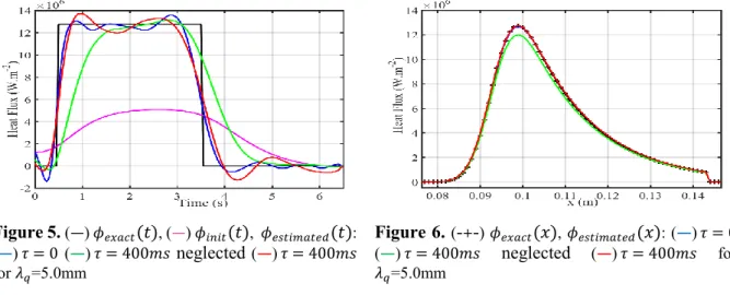
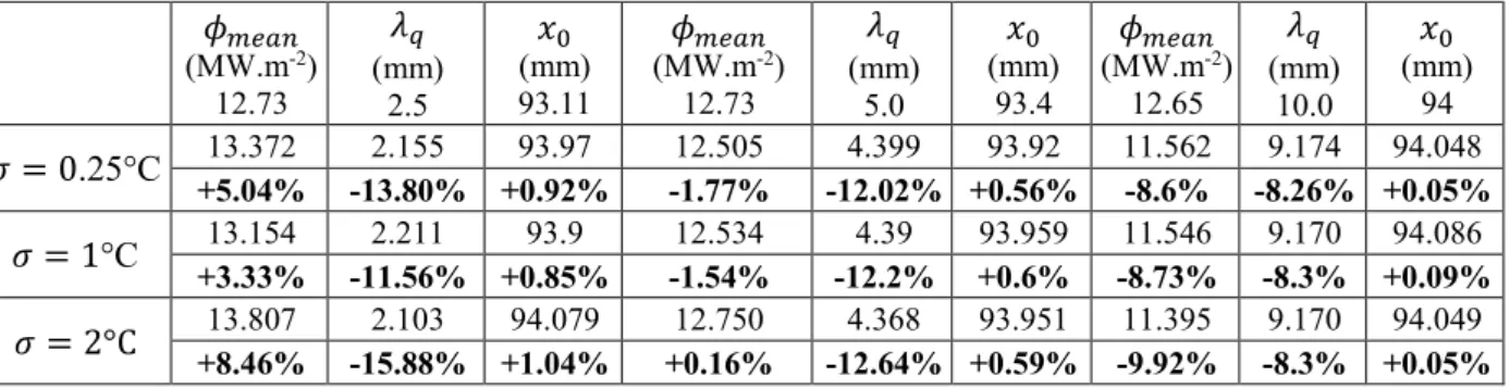
Figure 5 and 6 show the estimated heat fluxes function with respect to the time and the poloidal location x (focused on the heat flux region). We note respectively that the time dependence and the spatial distribution of identified heat fluxes are well recovered for all cases except when the synthetics measurement are computed with the TC response time 𝜏=400ms that is neglected for the inversion. In this case the step variations are delayed with the order of magnitude of 𝜏 but the spatial variation is still recovered thanks to the good estimations of 𝜆𝑞 and 𝑥0.
Table 1 summarizes the results for each values of 𝜆𝑞. We observe that the estimation of 𝜆𝑞 is done
with an error less than 3% for all cases and especially for 𝜆𝑞=2.5mm where the heat flux is the most peaked. 𝜙𝑚𝑒𝑎𝑛 is the average of the heat flux at the maximum location for 0.9<t<3.1s. These results show the accuracy of this approach to estimate the intensity of the heat flux and his decay length if we have the right a priori spatial distribution of the surface heat flux. We also notice that the time response of the TCs can be taken into account to improve the estimation of 𝜙𝑀(𝑡).
7th European Thermal-Sciences Conference (Eurotherm2016) IOP Publishing Journal of Physics: Conference Series 745 (2016) 032091 doi:10.1088/1742-6596/745/3/032091
Figure 5. (—) 𝜙𝑒𝑥𝑎𝑐𝑡(𝑡), (—) 𝜙𝑖𝑛𝑖𝑡(𝑡), 𝜙𝑒𝑠𝑡𝑖𝑚𝑎𝑡𝑒𝑑(𝑡): (—)𝜏 = 0 (—)𝜏 = 400𝑚𝑠 neglected (—)𝜏 = 400𝑚𝑠 for 𝜆𝑞=5.0mm Figure 6. (-+-) 𝜙𝑒𝑥𝑎𝑐𝑡(𝑥), 𝜙𝑒𝑠𝑡𝑖𝑚𝑎𝑡𝑒𝑑(𝑥): (—)𝜏 = 0 (—)𝜏 = 400𝑚𝑠 neglected (—)𝜏 = 400𝑚𝑠 for 𝜆𝑞=5.0mm
Table 1. Results of the estimation for all 𝜆𝑞 and 𝜏. Exact values are given in the first line. 𝜙𝑚𝑒𝑎𝑛 (MW.m-2) 12.73 𝜆𝑞 (mm) 2.5 𝑥0 (mm) 93.11 𝜙𝑚𝑒𝑎𝑛 (MW.m-2) 12.73 𝜆𝑞 (mm) 5.0 𝑥0 (mm) 93.4 𝜙𝑚𝑒𝑎𝑛 (MW.m-2) 12.65 𝜆𝑞 (mm) 10.0 𝑥0 (mm) 94 𝜏 = 0 +0.02% +1.12% 12.733 2.528 -0.1% 93.02 12.705 -0.2% +1.52% -0.04% 5.076 93.36 +0.06% 12.658 +2.52% +0.2% 10.252 94.19 𝜏 = 400𝑚𝑠 neglected 12.132 2.483 93.12 12.002 5.059 93.36 11.941 10.252 94.17 -4.7% -0.68% +0.01% -5.72% +1.18% -0.04% -5.6% +2.52% -0.18% 𝜏 = 400𝑚𝑠 12.931 2.491 93.07 12.747 5.071 93.36 12.613 10.276 94.15 +1.58% -0.36% -0.04% +0.13% +1.42% -0.04% -0.29% +2.76% +0.16% 5. Study of 3D effects
The objective of this section is to determine the accuracy of the present approach in predicting 𝜙(𝑥, 𝑡) using a 2D modeling for the inversion but using synthetics TC measurements generated with a 3D modeling. In this 3D modeling, the surface heat flux 𝜙(𝑥, 𝑦) is the output of the PFCFlux code [3] that takes into account the 3D geometry of the PFC and the magnetic equilibrium.
5.1. Synthetic measurements
The heat flux 𝜙(𝑥, 𝑦) is computed with the PFCFlux code in the FXP configuration for all values of 𝜆𝑞 at the mid-plane with the distribution of the equation 6 with 𝑓𝑥=1. As described in [3], PFCFlux is a
software dedicated to the calculation of the conducted power along the magnetic field lines assuming purely parallel transport (no cross-field transport) from the mid-plane to the PFC surface. Based on ray tracing techniques, it is able to simulate the magnetic shadowing between adjacent PFC’s. One of the particularity of this calculation is to take into account the variation of the magnetic field angle of incidence along the PFC which is not taken into account in the equation 6. The computed heat flux for 𝜆𝑞=5mm is shown in the figure 7 with the representation of the poloidal cross section of the 2D modeling, one can note at the bottom of the surface the shadowing (𝜙 =0 in blue) due to the previous PFC (about 3 mm). In addition, it appears also that the side of the PFC are not submitted to heat flux due to their shaping 2mm round edge.
Figure 8 shows in continuous lines the synthetics measurement generated with ANSYS in 3D using the heat flux computed with PFCFlux with the same time evolution as previously (step of 3s) and
𝜏=400ms. The dotted lines represent the synthetics measurement generated with ANSYS in 2D used before. As expected the discrepancies between the 3D and 2D modeling increase with time, the 3D heating is lower than the 2D one (about 10% after 3s) and the cooling rate is higher. This can be explained with the little wetted areas in the 3D modeling due to the shadowing effects and the PFC curved side (2mm round corner with no heat load).
7th European Thermal-Sciences Conference (Eurotherm2016) IOP Publishing Journal of Physics: Conference Series 745 (2016) 032091 doi:10.1088/1742-6596/745/3/032091
Figure 7. 𝜙(𝑥, 𝑦) (W.m-2) calculated by PFCFlux
for 𝜆𝑞=5.0mm at the mid-plane, white dotted line is the
cross section of the 2D modelling (TCs location)
Figure 8. simulated by ANSYS in 3D: (—) TCI (—
) TCMI (—) TCMO (—) TCO, simulated by ANSYS in 2D: (- - -) TCI (- - -) TCMI (- - -) TCMO (- - -) TCO all with 𝜏 = 400𝑚𝑠, 𝜎 = 1°𝐶 and 𝜆𝑞=5.0mm
5.2. Estimation results
We present here the results of the inversion using the 3D synthetics measurement for 𝜆𝑞=5mm with three levels of noise: 1) 𝜎=0.25°C, 2) 𝜎=1°C, 3) 𝜎=2°C. The initial guess of the parameters is set by the same way as previously: 𝜆𝑞=10mm, 𝑥0=80mm and 𝜙𝑀(𝑡) with a deconvolution method using the
TCMO measurements (magenta in figure 9) [9]. Figure 9 and 10 show respectively the estimated heat fluxes versus time and versus the poloidal location. We note that the dynamic is well recovered with a little under estimation of the heat flux about 2% and a little negative heat flux in the cooling phase to correct the higher inertial cooling of the 3D modeling. We can see the equivalent estimation with the different noise levels showing the robustness of the method in regard of noise measurements. Figure 10 shows also an under estimation of the 𝜆𝑞 of the heat flux for the three cases, this error is about 12% (4.4mm estimated instead of 5mm imposed in the PFCFlux code). Despite of the errors on 𝜆𝑞 and 𝜙𝑀(𝑡), the estimation of 𝑥0 is performed with a very little error (0.5%).
Figure 9. (—) 𝜙𝑒𝑥𝑎𝑐𝑡(𝑡), 𝜙𝑒𝑠𝑡𝑖𝑚𝑎𝑡𝑒𝑑(𝑡): (—)𝜎 =
0.25°𝐶(—)𝜎 = 1°𝐶 (—)𝜎 = 2°𝐶 for 𝜆𝑞=5.0mm
Figure 10. (—) 𝜙𝑒𝑥𝑎𝑐𝑡(𝑥), 𝜙𝑒𝑠𝑡𝑖𝑚𝑎𝑡𝑒𝑑(𝑥): (—)𝜎 =
0.25°𝐶(—)𝜎 = 1°𝐶 (—)𝜎 = 2°𝐶 for 𝜆𝑞=5.0mm Table 2. Results of the estimation for all 𝜆𝑞 and 𝜎. Exact values are given in the first line.
𝜙𝑚𝑒𝑎𝑛 (MW.m-2) 12.73 𝜆𝑞 (mm) 2.5 𝑥0 (mm) 93.11 𝜙𝑚𝑒𝑎𝑛 (MW.m-2) 12.73 𝜆𝑞 (mm) 5.0 𝑥0 (mm) 93.4 𝜙𝑚𝑒𝑎𝑛 (MW.m-2) 12.65 𝜆𝑞 (mm) 10.0 𝑥0 (mm) 94 𝜎 = 0.25°C 13.372 2.155 93.97 12.505 4.399 93.92 11.562 9.174 94.048 +5.04% -13.80% +0.92% -1.77% -12.02% +0.56% -8.6% -8.26% +0.05% 𝜎 = 1°C 13.154 2.211 93.9 12.534 4.39 93.959 11.546 9.170 94.086 +3.33% -11.56% +0.85% -1.54% -12.2% +0.6% -8.73% -8.3% +0.09% 𝜎 = 2°C +8.46% -15.88% +1.04% 13.807 2.103 94.079 +0.16% 12.750 -12.64% +0.59% -9.92% 4.368 93.951 11.395 -8.3% +0.05% 9.170 94.049 7th European Thermal-Sciences Conference (Eurotherm2016) IOP Publishing Journal of Physics: Conference Series 745 (2016) 032091 doi:10.1088/1742-6596/745/3/032091
Table 2 summarizes the results for each values of 𝜆𝑞. We observe that the estimation of 𝜆𝑞 is done with errors from 8.3% for 𝜆𝑞=10mm to 16% for 𝜆𝑞=2.5mm. This error has been quantified here for each parameter, in the range of expected values of 𝜆𝑞 including the 3D thermal effect (shadowing, wetted
area, finite size and shaping of the PFC). These results show that the assumptions of our model (2D, heuristic formulation for the spatial distribution of 𝜙) lead to acceptable errors on the estimated heat flux.
6. Conclusion
In this paper, 2D nonlinear unsteady calculations are used with the Conjugate Gradient Method and the adjoint state, for the heat flux estimation on the divertor graphite PFCs of the WEST tokamak. The combination of the heuristic target heat load profiles [6] (mainly constructed with IR thermography during Carbon-wall operation period) with an inverse heat flux calculation using the embedded TCs data, makes it possible the estimation of the maximum intensity 𝜙𝑀(𝑡), the decay length (𝜆𝑞) and the strike point location (𝑥0) of the surface heat flux on the divertor PFCs. It should be noted that no a priori information on the time evolution of the heat flux is needed for the estimation. This work is a positive evolution from previous studies [5] where only one embedded thermocouple was used for inversion making it mandatory knowledge of the true values of 𝜆𝑞 and 𝑥0. Here, the use of multiple embedded
thermocouples makes it possible to simultaneously identify 𝜆𝑞 and 𝑥0 together with 𝜙𝑀(𝑡).
Application to synthetics measurement generate with 2D modeling has been firstly introduced in order to study the accuracy of the method and the consideration of the time response of the TCs. We notice the good accuracy of this approach to estimate the intensity of the heat flux (< 2%) and his decay length (< 3%) if we have the right a priori heat flux spatial distribution. Finally we applied the method to synthetics measurement generated with 3D modeling and heat flux 𝜙(𝑥, 𝑦) calculated with a dedicated code (PFCFlux [3]) taking into account the shadowed and wetted areas of the PFC. The results showed that the assumptions of our model (2D, heuristic formulation for the spatial distribution of 𝜙) lead to acceptable errors on the heat flux estimation for the range of expected values of 𝜆𝑞 (errors on 𝜆𝑞 estimation go from 8.3% for 𝜆𝑞=10mm to 16% for 𝜆𝑞=2.5mm).
Acknowledgments
This work has been carried out thanks to the support of the A*MIDEX project (n°ANR-11-IDEX-0001-02) funded by the “Investissements d’Avenir” French Government program, managed by the French National Research Agency (ANR).
References
[1] Bourdell C et al 2015 WEST Physics Basis Nucl. Fusion 55 063017
[2] Bucalossi J et al 2014 The WEST project: Testing ITER divertor high heat flux component technology I a steady state tokamak environment Fusion Eng. Des. 89 907-12
[3] Firdaouss M et al 2015 Heat flux depositions on the WEST divertor and first wall components
Fusion Eng. Des. 98-99 1294-8
[4] Missirlian M et al 2014 The WEST project: Current status of the ITER-like tungsten divertor
Fusion Eng. Des. 89 1048-53
[5] Gaspar J et al 2013 Nonlinear heat flux estimation in the JET divertor with the ITER like wall Int.
J. Therm. Sci. 72 82-91
[6] Eich T et al 2013 Empirical scaling of inter-ELM power widths in ASDEX Upgrade and JET J.
Nucl. Mater. 438 S72-S77
[7] Colaco M-J et al 2001 Inverse convection problem of simultaneous estimation of two boundary heat fluxes in parallel plate channels J. Braz. Soc. Mech. Sci. 23 201-15
[8] Garnier B et al 2011 Measurements with contact in heat transfer: principles, implementation and pitfalls Advanced School on Thermal Measurements and Inverse Techniques (Roscoff) [9] Gardarein J-L et al 2013 Inverse heat conduction problem using thermocouple deconvolution:
application to the heat flux estimation in a tokamak Inv. Prob. Sci. Eng. 21 854-64
7th European Thermal-Sciences Conference (Eurotherm2016) IOP Publishing Journal of Physics: Conference Series 745 (2016) 032091 doi:10.1088/1742-6596/745/3/032091