HAL Id: hal-00022155
https://hal.archives-ouvertes.fr/hal-00022155
Submitted on 3 Apr 2006HAL is a multi-disciplinary open access
archive for the deposit and dissemination of sci-entific research documents, whether they are pub-lished or not. The documents may come from teaching and research institutions in France or abroad, or from public or private research centers.
L’archive ouverte pluridisciplinaire HAL, est destinée au dépôt et à la diffusion de documents scientifiques de niveau recherche, publiés ou non, émanant des établissements d’enseignement et de recherche français ou étrangers, des laboratoires publics ou privés.
Validity of the Diffused Aerial Image Model: an
Assessment Based on Multiple Test Cases
David Fuard, Maxime Besacier, Patrick Schiavone
To cite this version:
David Fuard, Maxime Besacier, Patrick Schiavone. Validity of the Diffused Aerial Image Model: an Assessment Based on Multiple Test Cases. 2003, pp.1536-1543, �10.1117/12.485516�. �hal-00022155�
Validity of the Diffused Aerial Image Model:
an Assessment Based on Multiple Test Cases
D. Fuard, M. Besacier, P. Schiavone, Laboratoire des Technologies de la Microélectronique CNRS,
c/o CEA Grenoble, 17 rue des Martyrs 38054 GRENOBLE cedex 9 France)
ABSTRACT
Lithography modeling is a very attractive way to predict the critical dimensions of patterned features after lithographic processing. In a previous paper[1], we have presented the assessment of three different simplified resist models (aerial image model, aerial image convolved with fixed gaussian noise and aerial image convolved with variable gaussian noise) by using a systematic comparison between experimental and simulated data. It has been shown that the aerial image convolved with fixed gaussian noise, or "diffused aerial image model" (DAIM), exhibits surprisingly good results of CD prediction for lines @ 193nm: using these datasets, the DAIM appears as a fast and accurate model for CD prediction. This approach allows also an easy run, and because it needs only four adjustable parameters, it avoids the difficult task of resist parameters extraction associated to full resist models, with.
In this paper, we enlarge the datasets used for the assessment of the DAIM by considering both lines and contact holes of various sizes printed at different wavelengths. The reference wafers have been printed at 248nm, 193nm and 157 nm. The procedure used to extract the model parameters has been improved and now needs less data to provide acceptable values. We will show that the validity of the DAIM extends well outside the results presented in ref. 1. Experimental data printed using various wavelengths, resists and exposure tools can be simulated accurately with CD prediction error ranging within few percents. It is to be noted that the results that will be presented on contact holes data indicate that the model is valid for 2D features. Finally, a comparison with full resist models shows that the accuracy of DAIM is comparable to more sophisticated and heavier models .
Keywords: Lithography simulation, simplified resist models, aerial image, CD prediction, gaussian noise, diffusion, OPC
1. INTRODUCTION
Two ways are used for CD prediction: full resist models (with physical meaning, but using a wider range of parameters), or simplified resist models (which empirically include all physical phenomena and use few model parameters). The problem of predicting critical dimensions (CD) of final patterned features using full resist models remains difficult and offers often sporadic results, because « the optimum performance of a simulation is only achieved by an appropriate determination of the model parameters and by a careful exploration of different modeling options »[2]. From the other side, a previous article shows that a DAIM, which consists in a convolution between the aerial image and a gaussian noise with a given full width at half maximum (FWHM), exhibits good performance in CD prediction for lines at 193 nm[1]. Historically, this approach, based on a diffusion of the aerial image using a convolution with a gaussian distribution, has been published by several authors for Optical Proximity Correction (OPC) purpose[3][4] In addition, Dolainsky and Maurer have proposed to use only four adjustable resist parameters for simple “diffused aerial image model”[4] The method presented here is a follow up of these two approaches.
The model that we use here needs only four parameters. In ref 1, for historical reasons, two of the model parameters where drawn separately from the isofocal dose of experimental data and isofocal threshold of the aerial image. Our experience has progressively shown that it was not the best solution. Especially when dealing with isolated features where the isofocal CD can be well outside the available data. An method of fit of the Bossung curve was put in place in order to overcome this problem. This fit was based on functions that rely on physical considerations and can include the isofocal dose or threshold as explicit coefficients.[5][6] This improved the reliability of the parameters extraction significantly. Nevertheless, we have still simplified the procedure by using a global optimization scheme where the four parameters are drawn together. This improved procedure is used in the following of this paper.
The aim of the work presented here is to assess whether this simple model could be applicable for all illumination condition (circle, annular, quadrupole), all mask designs (binary or phase shift masks ), for the widest range of feature
types (lines or contacts) and for all wavelengths ranging between 248 and 157 nm. In addition, a comparison of the results provided by this model and those provided by a full resist models using carefully determined model parameters, will complete that model reliability overview.
2. MODEL DESCRIPTION
This section reminds the basics of the Diffused Aerial Image Model and presents the procedure for the validity assessment. The available experimental data used, which are focus-exposure matrices, are presented in the following section. The data used in the present work are based on 248 nm, 193 nm and 157 nm resists.
2.1 Diffused Aerial Image Model
As already mentioned in the introduction, because FEM fitting expression includes dose (or threshold) at isofocal CD as coefficients, the previous procedure consists first in fitting experimental and simulated FEM for CD bias (∆CD), and doses and thresholds at isofocal CD finding. These last data allows the determination by regression (depictedFigure 1)
of the unambiguous relation dose a b
threshold
= + between experimental doses and aerial image intensity thresholds,
where a and b are constants.[1] Once, that relation is defined, the generation of simulated Bossung curves could be done with the aerial image intensity threshold corresponding to the experimental exposure doses of the experimental FEM. Then, a direct comparison of experimental and simulated FEM is possible and allows the calculation of the RMS error between real experiments and simulations. Finally, simulated FEM is generated for several gaussian noises σnoise convolution to find out the best match between experiments and simulation. This last comparison allows the determination of the last parameter σnoise. Once these four DAIM parameters (a, b, ∆CD, σnoise) are set, they could be used for CD prediction by the generation of simulated FEM. An achievement of our previous paper was also to show that the DAIM could be predictive . It has clearly been demonstrated that the model can simulate accurately CDs outside the set of data that had been used for fitting the model parameters.
The new procedure consists in an optimization which improves the four DAIM parameters (a, b, ∆CD, σnoise - described below and in the previous paper [1]) in the same time. The final simulated CD is optimized according to the expression:
, noise simul a CD CD AI f CD d b σ = + ∆ −
, (1) where:d and f are respectively the experimental exposure dose and defocus for which the CD is to be computed. -
noise
CD AIσ is the CD given by aerial image convolved with a gaussian distribution of σnoise half width. This CD is expressed as a function of the aerial image intensity threshold and the defocus f . This can be computed directly within the lithography simulator (in our case : Solid-C[9] + scanner noise setting). The CD is drawn from the aerial image at a given threshold. This threshold is related to the experimental exposure dose d by the expression a
d −b
This relation between experimental exposure dose and simulated intensity threshold has been detailed in Ref 1. It is based on the hypothesis that the resist has a threshold-like behavior[7, 8]. This kind of relation has to be used because the aerial image CD are expressed as a function of aerial image intensity, while experimental data are expressed as a function of exposure dose.
The a and b coefficients depend only of the given resist process (resist thickness, layer stack ,PEB an development conditions). They are of general use and they should be the same for all feature types, pitches, and optical settings. The σnoise parameter is not strictly speaking a diffusion coefficient, at this point it is only considered as an abstract value of “diffusion” which could include all types of diffusion occurring during exposure or post exposure bake for example. Physical meaning of this parameter is currently under investigation. Nevertheless, the simulated value found σnoise is not far from experimental diffusion lengths already published in the literature.[refs]
-- a
d −b is the equivalent aerial image intensity threshold expressed as a function of the exposure dose, to be
used to compute the CD from the diffused aerial image (simulator).
Moreover, other unknowns can be optimized at the same time without changing the methodology. For example, the adjustment of one or several unknown Zernike coefficients could be performed in addition to the extraction of the resist parameters..
3. MODEL ASSESSMENT BASED ON MULTIPLE TEST CASES
Our previous paper described the assessment of the DAIM with lines printed at 193 nm using Sumitomo PAR 707 resist. The DAIM error, determined by the mean CD discrepancy between experimental and simulated FEM data was found to be around 5%. These mean errors are summarized inTable 2, for all partial coherence and pitches conditions. It can be noted that the figures in Table 2differ slightly from those of Table 2 of Ref. 1. This is due to the use of the new procedure for optimizing the model parameters which provides here better CD errors.
The check of the validity of the DAIM for others lithographic conditions is lead with the experimental datasets described in paragraph 3.1. The improved parameter extraction procedure has been used.
3.1 Experimental datasets
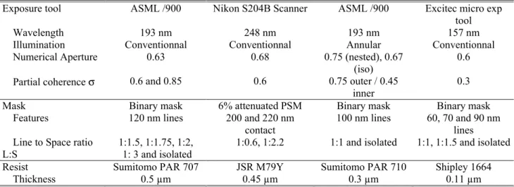
various wavelengths, masks (BIM and PSM), feature types (lines and contact holes), optical settings (numerical aperture and partial coherence), and illumination shapes (conventional and annular) have been used for the assessment. The available datasets on which we have performed a comparison between the DAIM results and measurements are listed below: The accuracy assessment of our simplified resist model has been lead using Focus Exposure Matrices (FEM). The simulated data are obtained using Solid C (from Sigma-C Gmbh). All experimental conditions are summarized in Table 1.
Contact holes @ 248nm :
The features were obtained using 0.45µm thick JSR M79Y resist , conventional illumination and 6% attenuated PSM. The nominal CD of the holes on the mask is 200 and 220 nm, with different space to line ratios S/L = 1:0.6 and 1:2.2. A Nikon S204B Scanner (248nm) stepper (0.68 numerical aperture, and partial coherence σ of 0.6) was used for the exposures. An Hitachi Critical Dimension Scanning Electron Microscope (Hitachi S9300 SEMCD top view) was used for evaluating the line CDs of developed resist features. No mask correction has been used in the simulations.
Lines @ 193nm :
The final features were obtained with 0.3µm thick Sumitomo PAR 710 resist on 82nm thick anti reflective coating AR19, using annular illumination (coherence of 0.75 outer / 0.45 inner) and binary masks, with an ASML/900 193nm stepper. The nominal CD of the lines on the mask are 100 nm, with nested lines (space ratio S/L = 1:1) and isolated lines. The numerical aperture are respectively 0.75 and 0.67 for dense lines and isolated lines.
Lines @ 157nm :
The final features were obtained with 0.11µm thick Shipley 1664 (prototype resist) on 117nm thick anti reflective coating AR19 and alternating PSM. The nominal CD of the lines on the mask are 90, 70 and 60 nm, with various line to space ratio S/L = 1:1, 1:1.5, and isolated lines. An 157nm Excitech micro stepper (0.6 numerical aperture, and partial coherence σ of 0.3) was used for the exposures. All the CD are measured via direct scanning electron microscopy views after cross-section.
3.2 Assessment of DAIM based on multiple test cases
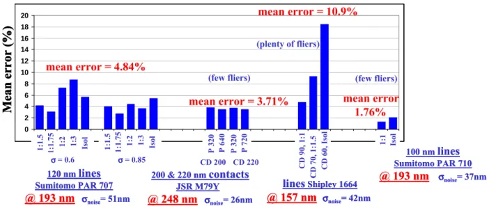
All the DAIM assessment for 248, 193 and 157 nm resist are respectively gathered together on Table 3, Table 5 and Table 4. These results of DAIM assessment show that this model exhibits very good CD predictions capabilities for all optical settings and all wavelengths ranging from 248 to 157 nm. Indeed:
1. the Table 3 shows that the DAIM CD prediction is very good for contact holes at 248 nm (JSR M79Y), with a
CD prediction error of less than 4% whatever considered CD or pitches. Two examples of superimposition of experimental datasets (dotted lines with diamonds) and best simulated CD prediction (solid lines) are shown Figure 3.
2. the Table 4 shows that the DAIM CD prediction errors remain also very good for lines at 193 nm (Sumitomo
of experimental FEM – CD prediction superimposition, depicted Figure 5, are on less noisy experimental datasets that those of Figure 3.
3. on other hand, 157nm lines CD predictions exhibits bad CD prediction errors, as shown in the Table 5. These bad CD prediction errors are associated with very noisy experimental datasets, as depicted Figure 4.
Finally, we can conclude that:
1. The DAIM fit RMS errors is greatly impacted by the noise of experimental data, and the best CD prediction,
the less noisier experimental datasets.
2. The DAIM CD prediction capability appears as real competitive one, with good mean CD prediction errors for
plenty of various experimental conditions. We can think that it remains the case for all possible experimental conditions. As the DAIM is a predictive model, it could be also used for CD prediction with others new illuminations conditions, using the four resist process DAIM parameters (which are set with basic illumination conditions experiments), for impact of high NA or high σ evaluation for example.
3.3 Comparison of DAIM CD prediction capabilities with full resist models
To check whether the DAIM is a competitive model compare to full resist models or not, we have used Steven G. Hansen results of full scalar and unpolarized vector models assessments. This work has been made using 193 nm lines of Sumitomo PAR 710 (cf. section 3.1). The final RMS errors between experimental and simulated FEM datasets, for all the models and pitches (nested 1:1 and isolated lines), are reported in the Table 6. In that table, we can see that the CD prediction of DAIM for isolated lines is very close from full resist models with about 2.1% RMS error, and appears with about 30% improvement for nested lines compare to full resist models (1.4% versus 2.1%, cf. Table 6). These results confirms that DAIM exhibits very good CD prediction capabilities compare both to full scalar and unpolarized vector full resist models. They also point out that DAIM could be a alternative to complex full resist models and appears to be reliable enough for CD prediction. In addition, the DAIM has got once again the main advantage to avoid difficult task of plenty complex full resist models parameters determination.
4. CONCLUSION
Full resist models are able to account for subtle physical phenomena, but the complex interplay of several effects make quantitative evaluation of the model parameters very difficult. In practice, the choice of best parameters can become subjective and these models sometimes loose one of their first purposes : accurate CD prediction. Like other simplified resist models, DAIM targets a different approach which consists only in good CD prediction capability with an easy and fast run, using only a small number of adjustable parameters.
The DAIM assessment has been based on multiple test cases. It has been shown that DAIM exhibits at least as good an accuracy as carefully adjusted full resist models for CD predictions. DAIM performs reasonably well for all illumination conditions, all mask designs (BIM or PSM), for the widest range of features (lines or contacts) and for all wavelengths ranging between 248 and 157 nm. It also exhibits good performance when applied to 2D features. Indeed, we have checked that a simple convolution of the aerial image with a gaussian noise distribution can overcome most of the limitations of the simple threshold model by adding one more “diffusion” adjustable parameter.
Along this work, it appeared to the authors that an objective assessment of resist models was not an obvious task. Moreover, from the literature, it was very difficult to have a clear idea of the real efficiency of a model (associated with its parameter settings). In order to clarify this point, it could be very useful to set up a kind of benchmark test (a set of common experimental data available to everybody) that should be referred to when a new model (or a parameter extraction technique) is published. The proper choice of an objective procedure is not trivial, but has to be thought about in order to save a lot of redundant effort.
ACKNOWLEDGMENTS
This work has been carried out within the European projects (MEDEA+ Fluor and IST UV2litho). The authors would like to acknowledge Elise Baylac, Yorick Trouiller and Serdar Manakli (from STMicroelectronics), Mieke Goethals and Jan Hermans (from IMEC), Steven Hansen for providing FEM data and full resist model results.
REFERENCES
1. D. Fuard, M. Besacier and P. Schiavone, "Assessment of different simplified resist models", SPIE Vol. 4691-136 (2001).
2. A. Erdmann, W. Henke, S. Robertson, E. Richter, B. Tollkühn, W. Hoppe, "Comparison of simulation approaches for Chemically Amplified Resists", Proc. SPIE Vol. 4404, pp. 99-110 (2001).
3. C.-N. Ahn, H.-B. Kim and K.-O. Baik, “A Novel Approximate Model for Resist Process”, SPIE Vol. 3334, pp.
752-763.
4. C. Dolainsky and W. Maurer, “Application of a Simple Resist Model to Fast Optical Proximity Correction”, SPIE
Vol. 3051, pp. 774-780.
5. S. A. Lis, “Micron and Submicron Integrated Circuit Metrology”, SPIE Vol. 565, pp. 143-151 (1985).
6. C. P. Außchnitt, “Rapid Optimization of the Lithographic Process Window”, SPIE Vol. 1088, pp. 115-123 (1989).
7. T. A. Brunner and R. A. Ferguson, "Approximate models for resist process effects", Proc. SPIE 2726, pp. 198-207 (1996).
8. J-Y. Yoo, Y-K. Kwon, J-T. Park, D-S. Sohn, S-G. Kim, Y-Su Sohn,"CD Prediction by Threshold Energy Resist Model (TERM)", Proc. SPIE Vol. 4690 (2002).
Exposure tool ASML /900 Nikon S204B Scanner ASML /900 Excitec micro exp tool
Wavelength 193 nm 248 nm 193 nm 157 nm
Illumination Conventionnal Conventionnal Annular Conventionnal
Numerical Aperture 0.63 0.68 0.75 (nested), 0.67
(iso)
0.6
Partial coherence σ 0.6 and 0.85 0.6 0.75 outer / 0.45
inner
0.3
Mask Binary mask 6% attenuated PSM Binary mask Binary mask
Features 120 nm lines 200 and 220 nm
contact
100 nm lines 60, 70 and 90 nm
lines Line to Space ratio
L:S
1:1.5, 1:1.75, 1:2, 1: 3 and isolated
1:0.6, 1:2.2 1:1 and isolated 1:1, 1:1.5 and isolated
Resist Sumitomo PAR 707 JSR M79Y Sumitomo PAR 710 Shipley 1664
Thickness 0.5 µm 0.45 µm 0.3 µm 0.11 µm
Table 1: Summary of the experimental datasets
σ Pitch (L:S) Error (whole set)
0.6 1 : 1.5 4.21 % 0.6 1 : 1.75 3.09 % 0.6 1 : 2 7.29 % 0.6 1 : 3 8.75 % 0.6 Isolated 5.72 % 0.85 1 : 1.5 4.05 % 0.85 1 : 1.75 2.78 % 0.85 1 : 2 4.42 % 0.85 1 : 3 3.72 % 0.85 Isolated 5.43 % Mean error 4.84 %
Table 2: Relative mean CD difference error between simulated and experimental data for 193 nm lines (Sumitomo PAR 707 resist)
CD (nm) Pitch (nm) Error (whole set)
200 320 3.88 %
200 640 3.57 %
220 320 3.81 %
220 720 3.57 %
Mean error 3.71 %
Table 3: Relative mean CD difference error between simulated and experimental data for 248 nm contact holes (JSR M79Y resist)
CD (nm) Pitch
(L:S)
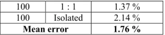
100 1 : 1 1.37 %
100 Isolated 2.14 %
Mean error 1.76 %
Table 4: RMS error between simulated and experimental data for 193 nm lines (Sumitomo PAR 710 resist)
CD (nm) Pitch (nm) Error (whole set)
90 1 : 1 4.77 %
70 1 : 1.5 9.35 %
60 Isolated 18.5 %
Mean error 10.9 %
Table 5: Relative mean CD difference error between simulated and experimental data for 157 nm lines (Shipley 1664 resist)
100nm dense lines (L:S = 1:1, NA = 0.75)
100nm isolated lines (NA = 0.67)
data subset: RMS error (nm) max error (nm) RMS error (nm) max error (nm)
full scalar model 2.06 3.87 2.27 6.03
unpolarized vector model 2.05 4.42 2.09 7.59
DAIM 1.37 3.20 2.14 6.20
0.4 0.5 0.6 0.7 0.8 6 8 10 12 14 0.6 ; 1.50 0.6 ; 1.75 0.6 ; 2.00 0.6 ; 3.00 0.6 ; .ISO 0.85 ; 1.50 0.85 ; 1.75 0.85 ; 2.00 0.85 ; 3.00 0.85 ; .ISO threshold at isofocal CD dose at isofocal CD (mJ.cm −2 )
Figure 1: Experimental exposure dose at isofocal CD vs. simulated intensity threshold at isofocal CD, for all experimental conditions (193 nm lines with Sumitomo PAR 707 resist) [1]
−0.4 −0.2 0 0.2 0.4 0.05 0.1 0.15 0.2 defocus (µm) CD ( µ m)
Figure 2: Superimposition of simulated CD (solid lines) and experimental FEM data (dotted lines with diamonds) for 120 nm lines at 193nm (Sumitomo PAR 707) using σ = 0.6, NA=0.63, and L:S = 1:1.5
−0.4 −0.2 0 0.2 0.4 0.1 0.15 0.2 0.25 defocus (µm) CD ( µ m)
Figure 3: Superimposition of simulated CD (solid lines) and experimental FEM data (dotted lines with diamonds) for 200 nm contact holes at 248nm using σ = 0.6, NA=0.68, and a pitch of 320 nm
−0.4 −0.2 0 0.2 0.4 0.02 0.04 0.06 0.08 0.1 defocus (µm) CD ( µ m) −0.4 −0.2 0 0.2 0.4 0.02 0.04 0.06 0.08 0.1 defocus (µm) CD ( µ m)
Figure 4: Superimposition of simulated CD (solid lines) and experimental FEM data (dotted lines with diamonds) for 70 nm nested lines 1:1.5 (left) and 60 nm isolated lines (right) at 157nm using σ = 0.3, NA=0.6
−0.4 −0.2 0 0.2 0.4 0.05 0.1 defocus (µm) CD ( µ m) −0.4 −0.2 0 0.2 0.4 0.05 0.1 defocus (µm) CD ( µ m)
Figure 5: Superimposition of simulated CD (solid lines) and experimental FEM data (dotted lines with diamonds) for 100 nm nested 1:1 (left) and isolated (right) lines at 193nm (Sumitomo PAR 710)
linesShipley 1664 @ 157 nm σσσσnoise= 42nm 100 nm lines Sumitomo PAR 710 @ 193 nm σσσσnoise= 37nm 0 2 4 6 8 10 12 14 16 18 20 mean error = 4.84% mean error = 3.71% mean error = 10.9% mean error 1.76% 1 :1 .5 1 :1 .7 5 1 :2 1:3 Is o l 1 :1 .5 1 :1 .7 5 1 :2 1:3 Is o l σσσσ= 0.6 σσσσ= 0.85 P 3 2 0 P 6 4 0 P 3 2 0 P 7 2 0 CD 200 CD 220 C D 9 0 , 1 :1
![Figure 1: Experimental exposure dose at isofocal CD vs. simulated intensity threshold at isofocal CD, for all experimental conditions (193 nm lines with Sumitomo PAR 707 resist) [1]](https://thumb-eu.123doks.com/thumbv2/123doknet/13038377.382255/9.892.286.613.197.446/experimental-exposure-simulated-intensity-threshold-experimental-conditions-sumitomo.webp)