Climate change and population: an integrated assessment of mortality due to health impacts

HAL Id: halshs-03048602

https://halshs.archives-ouvertes.fr/halshs-03048602

HAL is a multi-disciplinary open access archive for the deposit and dissemination of

sci-L’archive ouverte pluridisciplinaire HAL, est destinée au dépôt et à la diffusion de documents

Climate change and population: an integrated

assessment of mortality due to health impacts

Antonin Pottier, Marc Fleurbaey, Aurélie Méjean, Stéphane Zuber

To cite this version:

Antonin Pottier, Marc Fleurbaey, Aurélie Méjean, Stéphane Zuber. Climate change and population: an integrated assessment of mortality due to health impacts. 2020. �halshs-03048602�

Documents de Travail du

Centre d’Economie de la Sorbonne

Climate change and population: an integrated assessment

of mortality due to health impacts

Antonin P

Marc F

Aurélie M

Stéphane Z

Climate change and population: an integrated assessment of

mortality due to health impacts

Antonin Pottiera,⇤, Marc Fleurbaeyb, Aur´elie M´ejeanc, St´ephane Zuberd

a_{Centre International de Recherche sur l’Environnement et le D´eveloppement (CIRED),} EHESS, Nogent-sur-Marne, France.

b_{Paris School of Economics, CNRS, Paris, France.}

c_{Centre International de Recherche sur l’Environnement et le D´eveloppement (CIRED),} CNRS, Nogent-sur-Marne, France.

d_{Paris School of Economics, CNRS, Paris, France.}

Abstract

We develop an integrated assessment model with endogenous population dynamics ac-counting for the impact of global climate change on mortality through five channels (heat, diarrhoeal disease, malaria, dengue, undernutrition). An age-dependent endoge-nous mortality rate, which depends linearly on global temperature increase, is introduced and calibrated. We consider three emission scenarios (business-as-usual, 3 C and 2 C scenarios) and find that the five risks induce deaths in the range from 160,000 per annum (in the near term) to almost 350,000 (at the end of the century) in the business-as-annual. We examine the number of life-years lost due to the five selected risks and find figures ranging from 5 to 10 millions annually. These numbers are too low to impact the ag-gregate dynamics and we do not find significant feedback e↵ects of climate mortality to production, and thus emissions and temperature increase. But we do find interest-ing evolution patterns. The number of life-years lost is constant (business-as-usual) or decreases over time (3 C and 2 C). For the stabilisation scenarios, we find that the number of life-years lost is higher today than in 2100, due to improvements in generic mortality conditions, the bias of those improvements towards the young, and an ageing population. From that perspective, the present generation is found to bear the brunt of the considered climate change impacts.

JEL classification: Q51; Q54; J11

Keywords: Climate change, Impacts, Integrated assessment model, Mortality risk,

Endogenous population.

⇤_{Corresponding author.}

E-mail addresses: pottier@centre-cired.fr (A. Pottier), Marc.Fleurbaey@psemail.eu (M. Fleur-baey), mejean@centre-cired.fr (A. M´ejean), Stephane.Zuber@univ-paris1.fr (S. Zuber).

1. Introduction

Recent knowledge about climate change has revived old concerns about a pos-sible conflict between human development and population size. Greenhouse gas (GHG) emissions due to human activity (mainly productive activities) are widely acknowledged to be a key driver of climate change, as described in the late report of Working Group I of the Intergovernmental Panel on Climate Change (IPCC, 2013). The size of the human population, in the near-term and distant future, is a key determinant of climate policy. All else equal, a larger population entails more emissions and therefore more mitigation to achieve a given climate target. The link between population growth and greenhouse gas emissions has long been recognised (Gaffin and O’Neil, 1997; Kelly and Kolstad, 2001; O’Neill et al., 2010; O’Neil et al., 2012; Casey and Galor, 2017), and thus family planning has been mentioned as a possible way to mitigate climate change (Cafaro, 2012; Spears, 2015).

Climate change will in turn have strong impacts on human livelihoods, for instance through extreme events such as floods, droughts or heat waves (IPCC, 2012), or through the prevalence of some diseases (WHO, 2014). Climate change is thus expected to strongly a↵ect human health and mortality, and feedback on population. It will change its size and structure, it will impact human longevity. As argued by Amartya Sen (1998), mortality is a key indicator of economic success and human development. Similarly, economists and demographers have long underlined the importance of accounting for mortality changes when comparing standards of living across time (Usher, 1980; Williamson, 1984; Murphy and Topel, 2003; Becker et al., 2005).

In this perspective, this paper provides an evaluation in physical units of the e↵ects of climate change on population, its size and structure. Such an evaluation is a first step towards an assessment of the impact of climate change on human longevity and mortality, two fundamental dimensions of sustainable development. More precisely, we extend the integrated assessment model (IAM) RESPONSE with endogenous population dynamics based on the cohort-component method, that enables a precise description of the evolution of population by age and sex. To account for the impact of global climate change on mortality, we restrict our-selves to five causes of death (heat-related, diarrhoeal disease, malaria, dengue and undernutrition), that will be enhanced by climate change. For each of these risk, we introduce an age-dependent endogenous mortality rate, which is increas-ing with global temperature increase, and calibrate it on data from WHO (2014). Using RESPONSE, we examine the impact of climate change on population size and structure in three emission scenario (business-as-usual (BAU), 3 C and 2 C). We provide several aggregate measures in physical units of the impacts, tak-ing advantage of knowtak-ing them by age groups. One could imagine that climate

related mortality could decrease population, and therefore emissions and tem-perature increase. We find no evidence of such feedback e↵ects. We do however find interesting patterns regarding the evolution of mortality through time. The number of life-years lost is constant (business-as-usual) or decreases over time (3 C and 2 C). For the stabilisation scenarios, we find that the number of life-years lost is higher today than in 2100, due to improvements in generic mortality conditions, the bias of those improvements towards the young, and an ageing population. From that perspective, the present generation is found to bear the brunt of the considered climate change impacts.

This paper is organised as follows. In the section 2, we present the methods used to endogenize population and discuss the emission scenarios considered. In section 3, we present and discuss our results regarding the evolution of total

population, the number of climate change-related deaths1_{, the number of unborn}

people and the number of years of life lost. We disentangle how changes in population size and structure (inter alia) can explain the numbers. Section 4 concludes.

2. Methods

To produce our estimates, we built on the RESPONSE model (Dumas et al.,

2012; Pottier et al., 2015). RESPONSE belongs to the compact IAMs family2,

it considers a simple representation of the economy, where the production of a single good is derived from labour and capital inputs. Greenhouse gas emissions are a by-product of the productive process, that build up in the atmosphere. The resulting global temperature increase, which is computed thanks to a carbon cycle and climate modules, feedbacks on productive process through a damage function.

In previous versions of RESPONSE, as well as in leading IAMs, population growth is considered to be exogenous. In this paper, we adapt the RESPONSE model to include a population module that can endogenously represent popula-tion dynamics. We follow the UN populapopula-tion projecpopula-tions (2015b; 2015a) and use the cohort-component method to project population, which provides an account-ing framework for fertility, mortality and migrations. In this section, as other parts of RESPONSE are left unchanged, we focus on how we model population

1_{Those are the deaths provoked by climate change through the five mortality risks discussed} above. They are only a subset of all deaths caused by climate change as other risks (e.g. catastrophic events) should be taken into account for a comprehensive analysis.

2_{Such as DICE (Nordhaus, 1994, 2008), FUND (Tol, 1997; Antho↵ and Tol, 2012), PAGE} (Plambeck et al., 1997; Hope, 2006) or NICE (Dennig et al., 2015). Compact IAMs are based on simple economic growth models, in contrast with process-based IAMs.

dynamics and how we introduce a second feedback (through mortality) of global temperature increase on the socio-economic system.

We first review the cohort-component method to project population estimates and the UN data used in these projections. Second, we explain how we model a mortality risk due to climate change and how we calibrate the associated proba-bility of dying. Third, we present the scenarios considered.

2.1. The cohort-component method

The cohort-component method is the most common method to project population in the long run. Here we rely on the description of this method by Preston et al. (2001).

Generally speaking, evolution of population occurs through three events: death, birth, and migration. As RESPONSE is a global model, its population is closed and migration plays no role. We thus only need to describe how the cohort-component method accounts for deaths and births. However, one would have to tackle the thorny problem of modelling migration flows to obtain regional estimates. This is left for future research.

Population is organised by age and sex groups. Specifically, we divide popu-lation between males and females and five-year age groups. The oldest age group (or open-ended interval) is 80+ (80-year-olds and older people). The population

at time t is thus segmented into 2⇤ (16 + 1) = 34 subpopulations. Total

popu-lation at time t is the sum of these scalars. We will note N_xF(t) (resp. N_xM(t))

the number of females (resp. males) between age x and x + 5 at date t. From a description of population at time t in this form, the cohort-component method projects population at t + 5 (i.e. five years later), in the same form. The method can then be iterated to produce long-run estimates of population. To project population at time t + 5, one has to distinguish between age-groups above five years old (i.e. cohorts already alive at t), and the new born cohort under five

years old (i.e. N₀F(t + 5) and N₀M(t + 5)).

Projecting age-groups older than five is rather straightforward. The number

of people of age x and sex i at time t+5, Ni

x(t+5), is simply the number of people

of age x 5 at time t, N_{x 5}i (t) (which is the same cohort), times the survivorship

ratio, SVRi_x(t). The survivorship ratio3 is estimated as the proportion of people

aged between x 5 and x who will be alive five years later in a stationary

population, subject to the table at period t. This is simply the ratio of

life-years lived by the stationary population between age x 5 and x and life-years

lived by the stationary population between ages x and x + 5 (data provided by life-tables). Projecting age groups (male and female) younger than five involves three di↵erent steps.

1. The number of births B[t, t + 5] between t and t + 5 is estimated. To do so, the cohort-component method derives the number of births by women aged between x and x + 5 and sums them across all possible age-groups of mothers. The number of births given by the women aged between x and x + 5 is simply 5 (i.e. the time span between t and t + 5) times the fertility

rate Fx(t) at date t for women aged between x and x + 5 times the average

number of women aged between x and x + 5 during that period, which is

(N_xF(t) + N_xF(t + 5))/2. So the number of births is:

B[t, t + 5] = 5X x Fx(t)N F x(t) + NxF(t + 5) 2 (1)

2. Births are then allocated between male and female births according to the

sex ratio at birth at that period, SRB(t): BF_{[t, t + 5] = B[t, t + 5]/(1 +}

SRB(t)) and BM[t, t + 5] = B[t, t + 5].SRB(t)/(1 + SRB(t)).

3. The final number of individuals of sex i aged from 0 to 5 at date t + 5,

Ni

0(t + 5), is obtained by multiplying the number of births Bi[t, t + 5] by

the appropriate survivorship ratio SVRi

0(t).

Starting from an initial description of population, the cohort-component method thus projects future population using three types of data: life-tables, fertility rates and sex-ratios at birth. The UN World Population Prospect (WPP) provides the initial population and these data for each time period until 2100 (we used the data from the 2015 WPP). Starting from the population numbers given for 2015, we are then able to project world population up to 2100 by sex and five-year age group. We rely on data from the medium variant, as the life-tables required to implement the cohort-component method is available only for this variant. The medium-variant projection assumes a decline of fertility for countries where large families are still prevalent, leading to the near stabilisation of population during the twenty-second century. Indeed, it projects a human population of 9.6 billion in 2050 and 10.9 billion by 2100.

Although the UN WPP already provide world and regional projections, we need to implement the cohort-component method, so that we can reproduce UN WPP projections and modify them. Indeed, we will soon consider climate change impacts on mortality (and in future stages, on fertility). Once we introduce climate change-related mortality, the structure of the population (i.e. how it is distributed among age and sex groups) changes and deviates from the WPP projections. To correctly represent the impacts of climate change on population, it is necessary to take into account these first and second round e↵ects and so to to apply the cohort-component method to project the population.

Apart from the climate change-related mortality, we want fertility and mortal-ity conditions to be as close as possible to those used in UN projections. Indeed, the probability of dying and fertility rates provided by the WPP incorporate many di↵erent assumptions about socio-demographic evolutions (declining fertil-ity rates and child mortalfertil-ity, health improvements, etc...). Given that the focus of the paper is on climate change-related mortality, we do not want to modify the WPP projections outside this realm and we rely on these assumptions.

2.2. Climate change-related mortality

Climate change can impact the three aspects of demography: fertility, mortality and migrations. As migration is excluded from our global model, only fertility and mortality have to be considered.

In this first exploration of the demographic consequences of climate change, we focus on mortality. We deliberately abstract from any change on fertility, either direct fertility changes due to climate impacts or possible indirect fertility changes that may occur as ways to adapt to changing mortality conditions (e.g. the replacement e↵ect of child mortality on fertility). Two reasons may be put forward to justify this choice. First, mortality impacts of climate change seem better known than fertility impacts in general. Reviews of mortality impacts are available in the literature, see for instance Carleton and Hsiang (2016), but we lack a comprehensive review of fertility impacts. Second, the impacts on fertility of higher temperature are quite difficult to assess in the long-run as it will interfere with reproductive choices. For instance, although hot days or heat-wave have induced lower birth chances eight to ten months later in the US (Barreca et al., 2015), the subsequent rebound in fertility makes it difficult to assert that those induced a sustained reduction in fertility.

We rely on the review done by the WHO (2014) to model how climate change impacts mortality. The WHO (2014) study reports the total number of addi-tional deaths that can be attributed to climate change for five mortality risks: undernutrition (for children under 5), malaria (for all ages), diarrhoeal disease (for children under 15), dengue (for all ages) and heat (for people above 65). The WHO (2014) assessment uses scenarios to estimate the e↵ect of climate change on the five mortality risks mentioned above and on flood-related mortality risk (no numbers are provided for this risk which is more uncertain). Baseline future cause-specific mortality in 2030 and 2050 is estimated using regression methods. Then the assessment develop global climate-health models in a specific future climate change emissions scenario (SRES A1b). The annual burden of mortality due to climate change was estimated for world regions as the di↵erence between the baseline and climate change scenarios. Table 1 shows the number of deaths for these five risks aggregated at the world level, in 2050 for a SRES A1b scenario.

undernutrition malaria dengue diarrhoeal disease heat number

of deaths 84 697 32 695 282 32 955 94 621

Table 1: Additional deaths in 2050 attributable to climate change for five mortality risks (WHO, 2014)

Data are also provided at the regional level (see Appendix Appendix C).

Because we consider only these five risks, our climate change-related mortality is only a subset of the mortality really caused by climate change. Other risks could have been added to our framework, such as emergent viruses, conflicts, extreme events, etc. We could also have added some health co-benefits of emission reduction, for instance due to reduced air pollution. We have refrained from including these due to lack of data. Although there are data on these risk, we have not found global estimates decomposed by age-groups. For the same

reason, and although more recent study exist for the risk we consider,4 _{they do}

not include decompositions of the impacts by age group, while the age-structure of the population plays a key role for our result as we will show. We have therefore preferred keeping the scope of the WHO study rather than mixing estimates and educated guess. Note that our framework can readily incorporate other risks, as the data become available.

Without climate change-related mortality, life-tables at time t are computed

from an age- and sex-specific probability of dying q₅ i

x(t), which we call the

base-line probability of dying. With climate change-related mortality, we make the assumption that the probability of dying becomes:

˜ q 5 ix(t) = q5 ix(t). 2 41 + 0 @ X j2N(x) ↵j 1 A T✓ t 3 5 (2)

where the sum is taken over the five possible mortality risks j, N (x) is the set of risks relevant for the age group between x and x + 5 (for example, the age

group 10 15 is a↵ected by the risks of diarrhoeal disease, malaria and dengue,

conversely malaria a↵ects all age groups, whereas for example undernutrition

a↵ects only children under 5), Tt is the global temperature increase at time t, ↵j

is the relative increase in the probability of dying due to risk j at the calibration temperature increase. Parameter ✓ specifies the dependence of the probability

4_{See for instance Mora et al. (2017) for heat-related mortality, Caminade et al. (2014) for} malaria, or Hasegawa et al. (2016) for undernutrition.

of dying with respect to temperature. Several assumptions are embedded in the choice of this functional form. We discuss some of them below.

The total probability of dying is thus the sum of probability of dying pro-vided by the WPP and of climate change-related probabilities of dying. Climate change-related mortality risk is added above the baseline mortality risk. There-fore, our formula implicitly assumes that the baseline mortality risk of the WPP includes no specific mortality related to climate change. This is certainly the most reasonable assumption to start with, as the WPP does not mention any climate scenario in conjunction with their projections.

The climate change-related probabilities of dying are added as a percentage of

the baseline probability of dying. Specifically, at temperature increase Tt=1 C,

climate change-related mortality risk j increases the probability of dying by ↵j

percent. As a consequence, the climate change-related mortality risk follows the general temporal evolution of mortality risks as incorporated in the evolution

of q₅ i_x(t). This is a reasonable assumption, since climate change-related

mortal-ity will certainly be influenced by general sanitary conditions, health systems, availability of pharmaceutical drugs, all factors that are already reflected in the

evolution of q₅ i

x(t) over time t. This is the reason why we choose the climate

change-related probability of dying to be proportional to the baseline probability of dying.

The climate change-related mortality risk is age-specific. For each age group, we account for the di↵erent risks pertaining to that age group according to the WHO classification. Note however that for a single type of risk (e.g., malaria)

the percentage of risk added is not age- nor sex-specific. That is, the ↵j does not

depend on the age-group x nor on sex i. The relative increase of mortality risk

due to malaria is thus the same for the age-groups 10 15, 35 40 or 75 80.

This assumption is made for simplicity and is due to the lack of sufficient data to calibrate age-specific or sex-specific mortality risk for a given risk.

We assume that the risk increases with climate change and we use the global temperature increase (or anomaly) as a proxy for climate change. This is a crude assumption, as mortality is more likely to depend on more specific climate data. This assumption is made necessary because climate modules embedded in IAMs are of limited dimensions and generally restricted to temperature. We have chosen a power-dependence for temperature, akin to the usual damage functions used in the climate change economics literature. The dependence in temperature is the same for each risk, i.e. ✓ does not depend on risk j. This assumption simplifies the analysis of the sensitivity of the results to this parameter.

How do we calibrate the ↵j? The WHO study gives the number of additional

deaths for each mortality risk j in 2050 for the A1b scenario with the medium

population variant of the WPP. We use this number to calibrate the ↵j. From the

in 2050, with and without risk j, and compute the di↵erence in the number of

deaths. We then choose the ↵j so that this di↵erence in deaths matches the

number of additional deaths reported by the WHO study. We do so for the five types of mortality risks considered.

Life-table data is necessary to implement the cohort-component method. It is provided by the WPP in the exogenous scenario (i.e. without climate change-related mortality). Once we introduce climate change-change-related mortality, we

re-compute the life-table at each t using the current probability of dying ˜₅qi_x(t)

which includes the climate change-related risk (and thus depends on global tem-perature at t). We then apply the cohort-component method to project global population for a given climate scenario.

2.3. Projections under three emission scenarios

We compute projections of world population in seven model runs. The first run is the projection without climate change-related mortality risk. In that reference run, labelled exogenous population, population does not depend on any model variable. The other runs are defined by a combination of a climate scenario and a value of parameter ✓.

We consider three emission scenarios with endogenous population. In those runs, the size of the population has been made endogenous due to the introduction of a non-zero climate change-related mortality risk. The scenarios relate to three di↵erent emission trajectories. In the business-as-usual (BAU) scenario, there is no control of GHG emissions: the GHG stock builds up rapidly in the atmosphere and climate change is substantial. The 2 C and 3 C scenarios correspond to two stabilisation policies that control GHG emissions so as to stabilise global temperature increase. Emissions and temperature increase for the three scenarios are reported in Figure ??.

World population is projected for these three emission scenarios for two values of the dependence of risk with temperature (✓ = 1, 2), totalling six di↵erent runs with an endogenous population. The results presented in the following section assume a linear relationship between the climate change-related mortality and temperature increase (i.e., ✓ = 1), the sensitivity analysis on the value of that parameter is presented in Appendix Appendix B.

3. Results

The impacts of climate change on mortality can be aggregated and summed-up according to di↵erent metrics. The standard economic approach to measure mortality has been to use a value of a statistical life (VSL) to adjust per capita GDP (Gross Domestic Product). The public health literature, as well as the

ecological economics literature, usually refrain from using such monetary values and resort to the number of years lost as a metric for mortality change. Here we follow this route and provide several measures in physical units: the evolution of total population (section 3.1), the number of unborn people (section 3.2), the number of climate change-related deaths (section 3.3), and the number of years of potential life lost (section 3.4).

3.1. Total population

The impact of endogenizing the e↵ect of climate change on population is neg-ligible before year 2100, even in the BAU scenario. This is shown on figure 1, which presents the evolution of population over time from year 2015 to year 2100 for the three emission policies considered (BAU, 2 C, 3 C) and for the reference exogenous population run. The red line shows the exogenous population trend (reference run), which is the case where there is no mortality risk related to cli-mate change. The exogenous trend dominates the evolution of global population. This trend is driven by the assumptions embedded in the medium variant of the WPP regarding converging fertility levels that ensure the near stabilisation of population at the end of the century. Adding a mortality risks due to climate change only slightly changes this picture.

This result as implications for the existence of potential feedback e↵ects. One could imagine that climate related mortality could decrease population, and therefore emissions and temperature increase. But the change in popula-tion between the exogenous and endogenous situapopula-tion is too small to impact the aggregate dynamics. Therefore we do not find significant feedback e↵ects.

To get a better sense of how climate change-related mortality risks impact total population, we show on Figure 2 the di↵erence between the reference run (exogenous population) and the endogenous population runs. In the BAU sce-nario, the human population counts 20 million fewer individuals in 2100 than in the case where population evolves exogenously (where mortality impacts due to the five risks are not considered). This is a modest number, as it represents 0.2% of total human population in 2100. The direct e↵ect of premature mortality somehow cumulates over years as some people who died early cannot reproduce, increasing the gap between the actual population and the reference (exogenous) case. We now examine this e↵ect of unborn people before dealing with number of deaths.

3.2. The unborn

In order to elaborate a normative evaluation of the e↵ect of climate change on population, we examine the number of people not born. This number can only be defined against a counterfactual population. The first e↵ect to account for is the

7 7.5 8 8.5 9 9.5 10 10.5 11 11.5 2015 2020 2025 2030 2035 2040 2045 2050 2055 2060 2065 2070 2075 2080 2085 2090 2095 2100 po pu la ti on ( bi ll io n ind iv idu al s) exogenous 2°C 3°C BAU

Figure 1: Evolution of population over the 21st century

-20 -18 -16 -14 -12 -10 -8 -6 -4 -2 0 2015 2020 2025 2030 2035 2040 2045 2050 2055 2060 2065 2070 2075 2080 2085 2090 2095 2100 po pu lat io n ( m ill io n in div id u als ) 2°C 3°C BAU

Figure 2: Di↵erence in total population in endogenous population runs compared with the exogenous population reference run

following. If a person dies (here a woman, as births are considered as produced by women only in the “female-dominant” model that is usual in demography) because of climate change before the end of her reproductive life, the children that this person would have had are considered people unborn. The second e↵ect accounts for the unborn children of unborn people, the children of their children,

etc. In this paper, we consider all people who were unborn, either directly (the first e↵ect) or indirectly (the second e↵ect). In each five-year period, the number of unborn individuals is the gap between the total number of births in that period in a given run and the total number of births in that period in the reference run (labelled exogenous population).

As shown on Figure 3, the number of unborn individuals per year reaches 218 thousands in the BAU scenario at the end of the century and around 190 thousands in the 3 C and 2 C scenarios (197 and 184 respectively). These num-bers are obtained by subtracting the total number of births occurring in a given climate scenario to the total number of births occurring in the case of an exoge-nous population. Climate change increases mortality in all age cohorts, which results in a number of children unborn due to the fact that their parents died too young to reach procreation age. The numbers are very modest for the first three or four five-year periods, as then people are not born only because of the premature death of their potential parents. Those numbers then increase sharply as they come to include both those unborn because their potential parents died at a young age and those unborn because their parents were not born either.

0 50 100 150 200 250 2015-2019 2020-2024 2025-2029 2030-2034 2035-2039 2040-2044 2045-2049 2050-2054 2055-2059 2060-2064 2065-2069 2070-2074 2075-2079 2080-2084 2085-2089 2090-2094 2095-2099 un bo rn (tho us and s pe r ye ar) 2°C 3°C BAU

3.3. Deaths due to climate change

In the model, an individual has two di↵erent ways of dying: either through gen-eral mortality or through climate change-related mortality. In any age group, the number of deaths related to a specific cause of mortality is proportional to the probability of dying from that cause. Figure 4 shows climate change-related deaths over time for the BAU, 2 C and 3 C scenarios, assuming a linear

relation-ship between the additional mortality risk and temperature increase (✓ = 1)5_{. In}

that case, the number of deaths per annum due to climate change doubles over the century, from 160,000 in the near term to almost 340,000 at the end of the century in the BAU scenario. By contrast, they slightly increase in the 3 C sce-nario to 230,000. In the 2 C scesce-narios, they are overall relatively constant. They climb slowly from 160,000 to 180,000 in 2070 and slightly decrease afterwards to reach 176,000 at the end of the century.

Although the reported values seem large, they represent a small fraction of total mortality (up to 0.5 percent). Indeed, annual deaths from all causes range from around 60 million today to 100 million at the end of the century. As a consequence, total population is little a↵ected by the endogenous mortality risk in the coming century, as shown in the results presented above. This has the further consequence that the feedback of endogenous population on the economic path is also negligible. The five additional mortality risks are also moderate compared to others risks regularly assessed by the WHO. Deaths from air pollution are currently estimated at 7 million per annum, deaths from AIDS at 1.1 million per annum, and deaths from traffic accidents at 1.3 million per annum. Deaths from malaria are reported to be around 450,000 annually whereas 800,000 people committed suicide annually.

It may seem puzzling that despite global temperature increase, the number of climate change-related deaths does not increase in stabilisation scenarios. This possibility can be explained by the way the climate change-related probability of dying is modelled. As shown in Eq. (2), the climate change-related probability of dying is modelled as an age-specific proportion of the baseline probability of dying, a proportion that increases with the global temperature anomaly. As the baseline probability of dying decreases over time as health conditions improve, an increase in global temperature may not translate into an increase in climate change-related mortality. Climate change-related mortality only increases if the decrease in baseline mortality is not sufficient to compensate for the impacts of higher global temperatures on mortality. If the decrease in baseline mortality is sufficiently fast, climate change-related mortality may decrease despite climate change.

0 50 100 150 200 250 300 350 2015-2019 2020-2024 2025-2029 2030-2034 2035-2039 2040-2044 2045-2049 2050-2054 2055-2059 2060-2064 2065-2069 2070-2074 2075-2079 2080-2084 2085-2089 2090-2094 2095-2099 de aths (tho usa nd s pe r ye ar ) 2°C 3°C BAU

Figure 4: Climate change-related deaths per annum

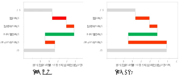
The composition of these two e↵ects is in reality more complicated as they also depend on the population structure. In order to better grasp the mecha-nisms driving these results, we propose a decomposition of the number of deaths related to climate change in two scenarios (2 C and BAU, see waterfall charts of Figure 5). Our decomposition is based on the four factors that contribute to the di↵erence between 2015 and 2100 climate change-related mortality: the population size, the age and sex structure, the projected temperature, and the general evolution of the (baseline) mortality risk.

We first consider this decomposition in the case of a 2 C scenario. The top bar of Figure 5a shows the number of annual deaths in 2015 as a starting point, the bottom bar showing the resulting number of deaths in 2100 when all e↵ects are accounted for. Each e↵ect is then added in turn as one browses down the figure, the length of the bar showing the number of additional deaths due to each particular e↵ect, and the colour of the bar signalling whether the e↵ect increases (in red) or reduces (in green) the number of annual deaths.

The first e↵ect considered relates to population size. Consider the counter-factual population with the population structure of 2015 and the population size of 2100. If the probability of dying as experienced in 2015 is applied to this coun-terfactual population, and still assuming 2015 temperatures, what would be the absolute number of additional deaths compared to 2015? The answer is given by the top red bar on the same figure. Unsurprisingly, a given probability of dying

0 50 100 150 200 250 300 350 400 2100 temperature of 2100 mortality of 2100 structure of 2100 size of 2100 2015

deaths due to climate change (thousands per year)

(a) 2 C 0 50 100 150 200 250 300 350 400 2100 temperature of 2100 mortality of 2100 structure of 2100 size of 2100 2015

deaths due to climate change (thousands per year)

(b) BAU

Figure 5: Decomposition of the number of annual deaths-related by climate change (2 C, BAU)

applied to a larger population entails a higher number of deaths (this is simply a scale e↵ect).

We then consider the population structure e↵ect. We assess its impact as the additional deaths between the counterfactual population just described and the population of 2100. Other things (than population structure) are held equal, and in particular we assume that the baseline mortality conditions and temper-ature are the same as those experienced in 2015. In that case, the ageing of the population means that less people are vulnerable to malnutrition and diarrhoeal diseases (which a↵ect children) related to climate change compared to the pop-ulation structure of 2015, whereas more people are vulnerable to heat (which a↵ects elderly people). In balance, the second e↵ect dominates, which explains the increase in the number of deaths (red bar).

The third component considered is the e↵ect of the evolution of the mortality risk over the century. That is we now apply to the population of 2100 the baseline probability of dying of that period (and not of 2015 as before) with the tempera-ture of 2015. The green bar on Figure 5 shows that the improvement of baseline mortality conditions (better sanitary conditions, health systems, availability of pharmaceutical drugs, etc.) is the e↵ect driving the slight decrease in the number of deaths in 2100 compared to 2015.

We finally consider the e↵ect of temperature alone, which is the last com-ponent to obtain the total additional number of deaths in 2100 compared to 2015. As the probability of dying depends linearly on temperature in our model, and considering that temperature is assumed to increase in 2100 compared to 2015 in the 2 C scenario, the temperature e↵ect increases the number of deaths

compared to the 2015 case. Overall, these e↵ects combined slightly reduce the number of annual deaths in 2100 compared to 2015. The picture is di↵erent in the BAU scenario (Figure 5b) where the temperature e↵ect is expectedly much larger than in the 2 C scenario (bottom red bar), leading to an overall increase in the number of annual deaths in 2100 compared to 2015.

3.4. Life-years lost due to climate change

We finally examine the number of life-years lost due to climate change. This is the number of deaths due to climate change in a given age group times the life-expectancy of that age-group (see discussion in appendix Appendix A). Com-pared to the number of deaths due to climate change, this amounts to weigh climate change-related deaths with the expected number of years that would re-main to the life of those dying prematurely. The number of life-years lost will be greatly a↵ected if death predominantly impacts the young or the old. In fact, in the case of climate change, additional deaths are concentrated among the young (0-15) and the old (65+).

The number of life-years lost ranges from 5 to 10 million per annum (Figure 6). Interestingly, the number of years lost is constant (BAU) or decreasing (3 C and 2 C scenarios) over time. Several e↵ects combine to produce this surprising result.

The first major e↵ect was discussed earlier when examining the number of deaths due to climate change. This number is constant in the 3 C and 2 C scenarios due to improving baseline mortality conditions. Moreover, according to WPP, the improvements of mortality conditions are expected to be greater for the young than for the old. As an example, the probability of dying at a young age is divided by more than 4 from 2015 to 2100, whereas the probability of dying at an old age (65+) is only divided by around 2 over the same time span. For a given population structure, this would thus reinforce the preponderance of old people among climate change-related deaths. The drastic improvements expected in terms of reduced child mortality between 2015 and 2100 translate into equally drastic improvements in terms of child mortality due to climate change, hence a great reduction in life-years lost.

The second major e↵ect is due to the change in the population structure (i.e. its age composition). Population is ageing, therefore climate change-related mortality increasingly concerns the elderly, simply because there will be more old people in the future. Indeed, the age-composition of the dead is reversed between the beginning and the end of the century. In 2015, 60% of overall deaths due to climate change concern children (0 to 5 years old), while in 2100, 50% of total deaths concern the elderly (over 80 years old).

0 2 4 6 8 10 12 2015-2019 2020-2024 2025-2029 2030-2034 2035-2039 2040-2044 2045-2049 2050-2054 2055-2059 2060-2064 2065-2069 2070-2074 2075-2079 2080-2084 2085-2089 2090-2094 2095-2099 li fe -ye ar s lo st (m il li ons pe r ye ar ) 2°C 3°C BAU

Figure 6: Life-years lost per annum due to climate change

striking. According to our results, in a stabilisation policy such as a 2 C scenario, there would be more life-years lost due to climate change now than at the end of

the 21st century. Indeed, when we consider the number of life-years lost, those

bearing the brunt of climate change impacts belong to the present generation,

not to future ones6_.

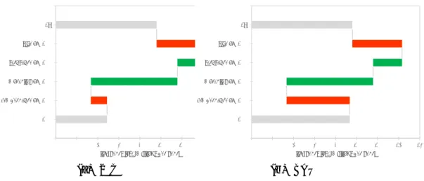
Again, we propose a decomposition of the number of life-years lost due to climate change in two scenarios (2 C and BAU), according to the various e↵ects that may drive the di↵erence in terms of life-years lost between 2015 and 2100 when endogenizing the e↵ect of climate change on mortality (Figure 7). We first consider this decomposition in the case of a 2 C scenario. The top bar of Figure 7a shows the number of life-years lost in 2015 as a starting point, and each e↵ect is considered in turn.

The first e↵ect relates to population size: we apply the probability of dying as experienced in 2015, still assuming 2015 temperatures, to the counterfactual population with structure of 2015 but with the size of the population in 2100. The result expectedly shows an increase in the number of life-years lost compared to the case with 2015 population size: a larger population simply entails a larger

6_{Note that focusing on monetary estimates would have delivered a di↵erent picture. Indeed} the absolute monetary value of these decreasing life-years lost actually increases, because of rising GDP. This reminds us that monetary estimates have to be put into perspective.

0 2 4 6 8 10 12 14 16 2100 temperature of 2100 mortality of 2100 structure of 2100 size of 2100 2015

life-years lost (millions per year)

(a) 2 C 0 2 4 6 8 10 12 14 16 2100 temperature of 2100 mortality of 2100 structure of 2100 size of 2100 2015

life-years lost (millions per year)

(b) BAU

Figure 7: Decomposition of the number of life-years lost due to climate change (2 C, BAU)

number of life-years lost annually.

We then consider the population structure e↵ect, by moving from the coun-terfactual population to the population of 2100. The ageing of the population between 2015 and 2100 means that the deaths due to climate change concern more the elderly in 2100 than in 2015, all other things being equal. We have seen previously that the population structure e↵ect implies actually more deaths. However, those deaths are mainly of old people and so are associated with a smaller number of life-years lost compared with the deaths of the young. So, despite an increase in overall deaths, the switch of death from young to old re-duces the number of life-years lost through this channel between 2015 and 2100 (green bar), in contrast with what happens for the number of deaths. This is the first e↵ect which explains the overall reduction of the number of life-years lost between 2015 and 2100.

The evolution of the mortality risk over the century is the second e↵ect driving the decrease in the number of life-years lost in 2100 compared to 2015. The green bar on Figure 7a shows that the improvement of baseline mortality conditions is the main driver of this reduction, because, as explained above, it greatly reduces mortality and does so more for young people (hence a greater reduction in life-years lost).

We finally consider the e↵ect of temperature alone. In the 2 C scenario, the global temperature is still assumed to be higher in 2100 than in 2015, increasing the number of life-years lost, all other things being equal. Overall, these e↵ects combined greatly reduce the number of life-years lost in 2100 compared to 2015. The picture is di↵erent in the BAU scenario (Figure 7b) where the

tempera-ture e↵ect is expectedly much larger than in the 2 C scenario (bottom red bar), leading to only a tiny decrease in the number of life-years lost annually in 2100 compared to 2015.

4. Conclusion

This paper provides an assessment of the e↵ect of climate change on future ulation projections using an integrated assessment model with endogenous pop-ulation dynamics. We examined three emission scenarios and showed that the projected impacts are modest, with a decrease of at most 0.5 percent of world population at the end of the century due to the five additional mortality risks enhanced by climate change (heat, diarrhoeal disease, malaria, dengue, undernu-trition). We also brought to the fore important metrics for a normative analysis: the number of deaths related to climate change, the number of life-years lost and the number of unborn people.

In a nutshell, we found the the aggregate mortality number are too low to generate feedback e↵ects. We however found interesting evolution patterns. We showed that climate change-related deaths per annum rise over time in the BAU, but are relatively constant (or slightly decreasing) in the 3 C and 2 C scenarios. These absolute values of the number of deaths due to the five risks considered are large, but they represent only a small fraction of total mortality (up to 0.5 per-cent), so that total population is not much a↵ected by the endogenous mortality risk over the next century. The deaths due to climate change are concentrated among the young and the old. The number of life-years lost ranges from 5 to 10 millions in a given year, depending on the date and scenarios. Interestingly, the number of life-years lost is constant (BAU) or decreasing (3 C and 2 C scenarios) over time due to changes in the age-composition of future population: population is ageing so that the additional mortality risk concerns more and more the elderly, hence reducing the number of years lost. This result is also explained by future improvements in baseline mortality conditions which are expected to be greater for the young than for the old, hence reduce the number of life-years lost.

We performed sensitivity tests regarding the impact of temperature increase on the added mortality risk due to climate change (section Appendix B),which shows that, although the numbers change, the qualitative picture is similar. We have also performed sensitivity tests regarding the regional disaggregation of the model: Section Appendix C shows that, although regional disparities exist (both in terms of the mortality level and of the time pattern), our aggregate results are rather robust.

The most striking result is that in climate stabilisation scenarios, the number of life-years lost because of climate change is actually higher today than at the end of the century. This stems for a conjunction of factors: the improvement

in mortality conditions that also reduces the number of deaths due to climate change (according to the way we modelled the dependence of mortality on tem-perature increase), a bias of these improvements towards young generations who are predominantly a↵ected by climate change-related mortality today, and an ageing population. Although using other data or incorporating additional risks will change the quantitative estimate and may increase its magnitude, this qual-itative result is robust to change in calibration as it depends on the functional form that models the climate change-related probability of dying. From a mor-tality perspective, according to our results, those bearing the brunt of climate change impacts are the present generation, not future ones.

This first attempt on examining the interaction between climate change, eco-nomics and demography opens several avenues of research. In our view, two issues are most pressing. The first is the policy implication of our results. Should these results change our view on mitigation policies? Do they alter the social cost of carbon? These questions are not easy to answer, as they imply to choose a normative view regarding, inter alia, how we value premature mortality. Second, we have not fully endogenized the population dynamics, and one could imagine that both mortality and fertility patterns could change as a response to climate mortality and climate damages. This would require new model developments that are beyond the scope of this paper. Similarly, the e↵ects of climate change on migrations could be studied using the integrated approach developed in this paper. And of course our results could be improved by including newer esti-mates and other causes of death (epidemics, conflicts, extreme weather events, air quality, etc.).

Acknowledgements

We thank John Broome, Victor Court, Florent MacIsaac, Noah Scovronick, and participants to the Endogenous Population Dynamics and Climate Change ses-sion at WCERE 2018 for their comments and suggestions.

This research has been supported by the ANR project FairClimpop, Grant # ANR-16-CE03-0001-01.

Appendix A. Computation of the number of life-years

lost

The aim of this appendix is to explain how we compute the number of life-years lost each year due to climate change. To do so, we introduce some general notations.

total population at time t is thus R₀1N (t, x)dx. The number of people born at exact time t is N (t, 0).

The population faces a mortality risk. One way to characterise this risk is to introduce the force of mortality. The force of mortality µ(t, x) is the instantaneous death rate at exact time t for individuals aged exactly x. In mathematical terms, it is:

µ(t, x) = N (t, x)˙

N (t, x) (A.1)

where ˙N (t, x) indicates the derivative of the function: h_{7! N(t + h, x + h) at}

point 0. With this definition, we can remark that the number of people aged x dying at time t is µ(t, x)N (t, x) [or between time t and t + dt is µ(t, x)N (t, x)dt].

So that the number of death at time t is R₀1µ(t, x)N (t, x)dx.

To simplify the computation of the number of year-life lost due to climate change, we first suppose that the force of mortality is stationary (section Ap-pendix A.1). We deal with the general case when the force of mortality depends on time in section Appendix A.2.

Appendix A.1. Stationary population

When the force of mortality is stationary, it does not depend on time t but only

on age x: µ(t, x) = µx. In the stationary case, we can integrate equation (A.1),

as

N (t, x) = N (t x, 0)e R0xµada

The number of people aged x at time t is the product of the number of people

born at time t x times a survival coefficient e R0xµada. Thanks to the stationarity

assumption, the survival coefficient depends only on the force of mortality and age x but not on time.

We furthermore suppose the number of new born N (t, 0) is constant over time equal to N , so that we have a stationary population model. A stationary population is remarkable as it is constant through time and keeps the same age structure. Furthermore, the structure of a given cohort, born at the same exact date, through time is the same as the age-structure of the population at a given time.

The life expectancy at birth of the cohort born at time t is equal to the number of life-year lived by the cohort divided by the cohort size. Because the mortality rate is stationary, it is independent of the time of birth. For a stationary population, it can also be computed as the ratio of total population at a given

time to new born. It can be written as:

e0=

Z ₁

0

dte R0tµada

More generally, the life-expectancy at age y (that is conditional on survival at age x) is:

ex=

Z ₁

x

dte Rxtµada

In the situation dealt with in the article, we have two di↵erent ways to exit the population (technically, this is a multi-decrement process): the first one is to die except from climate change related causes, the second is to die from causes

related to climate change. There are correspondingly two forces of mortality µ1

and µ2_{, that add up to make the total force of mortality µ}1+2 _{= µ}1_{+ µ}2_{. In the}

terms of the article, µ1 is the generic mortality whereas µ2 is the specific climate

related mortality that we introduced.

We can now compute the number of life-year lost because of climate change

(mortality process 2). The number of people aged x is N e R0xµ

1+2

a da_{. These}

dying at this age from climate change are in number: µ2

xN e Rx

0 µ 1+2

a da_{. What}

is the number of life-year lost by the premature death of these people because of climate change? Had they faced mortality risk 1 only, they would have live

expectedly another e1

x=

R₁

x dte Rt

xµadayears. The loss of expected life-years for

people aged x amounts to:

µ2_xN e R0xµ1+2a da

Z ₁

x

dte Rxtµ1ada

Therefore the total loss of expected life-years is:

Z ₁ 0 dxµ2_xN e R0xµ 1+2 a da Z ₁ x dte Rxtµ1ada _(A.2)

With this method to compute the number of expected life-year lost due to climate change, we have in fact reported at time t the life-year lost for the people who die prematurely at time t because of climate change. Another method is to report the expected loss of life-years for the people who are born at time t. This is the number of people being born N times the di↵erence in life-expectancy for mortality risk 1 only and life-expectancy for both mortality risks, i.e.

Z ₁

0

dxN⇣e R0xµ1ada _e

Rx

0 µ1+2a da⌘ _(A.3)

These two di↵erent methods are actually equivalent: when the population is stationary, the quantities (A.2) and (A.3) are equal. Indeed, starting from (A.2),

it can be rewritten as: Z ₁ 0 dxµ2_xN e R0xµ2ada Z ₁ x dte R0tµ1ada

which becomes after a partial integration =  N e R0xµ2ada Z ₁ x dte R0tµ1ada 1 0 Z ₁ 0 dxN e R0xµ2ada_e Rx 0 µ1ada =N Z ₁ 0 dte R0tµ1ada Z ₁ 0 dxN e R0xµ1+2a da

The last quantity is (A.3).

Appendix A.2. General case: non-stationary population

The general case is a little bit more complicated for two reasons: the force of mortality is no longer constant across time and the number of new born may vary across time. We therefore have to keep the two indices which makes notations cumbersome and manipulations harder to follow. But the logic is still the same.

By construction of the force of mortality, we have N (t, x) = N (t x, 0)e R0xµ(t x+a,a)da.

Life-expectancy at time t for those aged x is7:

ex(t) =

Z ₁

x

dse Rxsµ(t x+a,a)da

We now consider that there are two ways to exit the population, and two forces

of mortality µ1 _{and µ}2_{. Process 2 corresponds to die because of climate-change}

related causes.

When we compute the number of life-year lost at time t because of climate change, we still have two possibilities: to compute the expected life-year lost of those die at time t because of climate change or to compute the reduction of life-year lived by those who are born at time t. Contrary to the stationary population case, the two quantities will be di↵erent in general, but the two methods are still equivalent, in a way.

7_{This is sometimes named the cohort life-expectancy as it applies to a given cohort (the} people born at time t x). To be computed, it uses the force of mortality that this cohort will actually experience in the future. A quantity that is more common in demographics (because it relies only on quantities that can be measured today) is the period life-expectancy. It is the life-expectancy of the fictitious cohort experiencing the mortality conditions prevailing at date t, that is µ(t, x): ePx(t) =

R1 x dse

Rs xµ(t,a)da_.

Recording life-year loss at time of death

At time t, consider the people aged x. Their number is N (t, x) = N (t

x, 0)e R0xµ1+2(t x+a,a)da. The number of these people dying because of climate

change (mortality process 2) is µ2(t, x).N (t, x). Without climate change, they

would have lived, in expectancy, for e1_x(t) =R_x1dse Rxsµ1(t x+a,a)da more years.

So the number of life-year lost because of climate change by those dying at age x at time t is:

µ2(t, x)N (t, x)e1_x(t) (A.4)

The total number of life-year lost at time t by the premature deaths related to climate change is the sum of this quantity over age x. Hence:

Z ₁

x=0

dxµ2(t, x)N (t, x)e1_x(t) (A.5)

This is the quantity we discuss in the main text (section 3.4) and especially report in graph 6.

Recording life-year at time of birth

The alternative possibility is to record the life-year lost for the new born. For the cohort born at time t, of size N (t, 0), the number of life-year loss because of climate change is simply the size of the cohort times the di↵erence of life-years live between the mortality risk 1 and mortality risks 1 + 2:

N (t, 0) Z 1 0 dx⇣e R0xµ1(t+a,a)da e Rx 0 µ1+2(t+a,a)da ⌘ (A.6) This quantity will not be the same as the quantity (A.4). The two methods are however equivalent in a sense. They indeed compute the same number of life-year loss but only allocate them di↵erently across time. To see that, consider precisely the cohort born at time t. The method recording at time of birth will compute the quantity (A.6) once. The method recording at time of death will record the life-year loss through all times after t. At time t + x, the number of

life-year lost due to cohort born at time t will be µ2(t + x, x)N (t + x, x)e1_x(t + x).

The integration over all possible age of death x is the same quantity as (A.6). Indeed,

Z ₁ x=0 dxµ2(t + x, x)N (t + x, x)e1_x(t + x) = Z ₁ x=0 dxµ2(t + x, x)N (t, 0)e R0xµ1+2(t+a,a)da Z ₁ x dse Rxsµ1(t+a,a)da = Z 1 x=0 dxµ2(t + x, x)N (t, 0)e R0xµ2(t+a,a)da Z 1 x dse R0sµ1(t+a,a)da =  N (t, 0)e R0xµ2(t+a,a)da Z ₁ x dse R0sµ1(t+a,a)da 1 x=0 Z ₁ 0 dxN (t, 0)e R0xµ2(t+a,a)da.e Rx 0 µ1(t+a,a)da =N (t, 0) Z ₁ 0 dse R0sµ1(t+a,a)da Z ₁ 0 dxN (t, 0)e R0xµ1+2(t+a,a)da

This is precisely the quantity (A.6), which proves our claim.

The two methods will thus deliver the same cumulative number of life-year lost, but this are allocated di↵erently across time.

Appendix B. Sensitivity analysis on the dependence of

risk on temperature

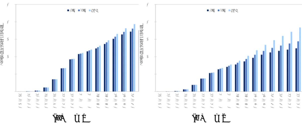
This section presents a sensivity of the results on the dependence of the added mortality risk on temperature (✓). We chose a power dependence of the added risk on temperature (cf. equation 2), akin to the usual damage functions used in the climate change economics literature.

Figure B.8 shows the evolution of population over time from year 2015 to year 2100 for the three emission policies (BAU, 2 C, 3 C) and the reference exogenous population run. The black dashed line shows the exogenous population trend (reference run), i.e. the case where there is no climate change-related mortality risk.

We show on Figure B.9 the di↵erence between the reference run (exogenous population) and the endogenous population runs. The largest decrease in human population compared to the counterfactual exogenous population scenario occurs in the BAU scenario when ✓ = 1.

The number of unborn people (Figure B.10) delivers a similar picture. The number of unborn people is higher for ✓ = 1 than for ✓ = 2 due to higher mortality in the first periods. As the e↵ect compounds over year, a steady increase after 2050 for ✓ = 2 is not sufficient to catch the number of unborn people for ✓ = 1.

7 7.5 8 8.5 9 9.5 10 10.5 11 11.5 2015 2020 2025 2030 2035 2040 2045 2050 2055 2060 2065 2070 2075 2080 2085 2090 2095 2100 po pu la ti on ( bi ll io n ind iv idu al s) exogenous 2°C 3°C BAU (a) ✓ = 1 7 7.5 8 8.5 9 9.5 10 10.5 11 11.5 2015 2020 2025 2030 2035 2040 2045 2050 2055 2060 2065 2070 2075 2080 2085 2090 2095 2100 po pu la ti on ( bi ll io n ind iv idu al s) exogenous 2°C 3°C BAU (b) ✓ = 2

Figure B.8: Evolution of population over the 21st century for two values of the de-pendence of the probability of dying with temperature (✓)

The di↵erence between the case ✓ = 1 and the case ✓ = 2 is even more striking when we consider the cumulated number of people not born over the period 2015-2100. When ✓ = 1, the cumulated number of unborn people reaches 9.4 million in the BAU scenario, 8.9 million in the 3 C scenario and 8.9 million in the 2 C scenario, higher than the case ✓ = 2 where it amounts to 6.8 million for the BAU scenario, 6.0 million for the 3 C scenario and 5.4 million for the 2 C scenario.

-20 -18 -16 -14 -12 -10 -8 -6 -4 -2 0 2015 2020 2025 2030 2035 2040 2045 2050 2055 2060 2065 2070 2075 2080 2085 2090 2095 2100 po pu lat io n ( m ill io n in div id u als ) 2°C 3°C BAU (a) ✓ = 1 -20 -18 -16 -14 -12 -10 -8 -6 -4 -2 0 2015 2020 2025 2030 2035 2040 2045 2050 2055 2060 2065 2070 2075 2080 2085 2090 2095 2100 po pu lat io n ( mil lio n in div id u als ) 2°C 3°C BAU (b) ✓ = 2

Figure B.9: Di↵erence in total population compared with the exogenous population case for two values of the dependence of the probability of dying with temperature (✓)

When the additional probability of dying is considered to be relatively sensi-tive to temperature increase (✓ = 2), climate-change related deaths per annum range from 85,000 to more than 0.5 million in the BAU (Figure B.11). They are moderately increasing in the 3 C and 2 C scenarios (from 85 thousands to

0 50 100 150 200 250 2015-2019 2020-2024 2025-2029 2030-2034 2035-2039 2040-2044 2045-2049 2050-2054 2055-2059 2060-2064 2065-2069 2070-2074 2075-2079 2080-2084 2085-2089 2090-2094 2095-2099 un bo rn (tho us and s pe r ye ar) 2°C 3°C BAU (a) ✓ = 1 0 50 100 150 200 250 2015-2019 2020-2024 2025-2029 2030-2034 2035-2039 2040-2044 2045-2049 2050-2054 2055-2059 2060-2064 2065-2069 2070-2074 2075-2079 2080-2084 2085-2089 2090-2094 2095-2099 unb or n (tho usa nd s pe r ye ar ) 2°C 3°C BAU (b) ✓ = 2

Figure B.10: Number of unborn people per annum due to climate change for two values of the dependence of the probability of dying with temperature (✓)

233 and 136 respectively). Over the first half of the century, the number of climate-change related deaths is higher in the case ✓ = 1 than in the case ✓ = 2 because the probability of dying is in fact lower in the case ✓ = 2. This may seem paradoxical, as when ✓ = 2, the relationship between mortality and temperature is more convex, but this is necessarily so, as long as the temperature increase remains below the temperature at the calibration point (2050) (the probabilities of dying are equal at the calibration point).

0 100 200 300 400 500 600 2015-2019 2020-2024 2025-2029 2030-2034 2035-2039 2040-2044 2045-2049 2050-2054 2055-2059 2060-2064 2065-2069 2070-2074 2075-2079 2080-2084 2085-2089 2090-2094 2095-2099 de aths (tho usa nd s pe r ye ar) 2°C 3°C BAU (a) ✓ = 1 0 100 200 300 400 500 600 2015-2019 2020-2024 2025-2029 2030-2034 2035-2039 2040-2044 2045-2049 2050-2054 2055-2059 2060-2064 2065-2069 2070-2074 2075-2079 2080-2084 2085-2089 2090-2094 2095-2099 de aths (tho us and s pe r ye ar ) 2°C 3°C BAU (b) ✓ = 2

Figure B.11: Climate change-related deaths per annum for two values of the depen-dence of the probability of dying with temperature (✓)

Again for life-years lost (Figure B.12), the number starts lower in the case ✓ = 2, than for ✓ = 1 because the climate change-related mortality risk is lower, but again life-years lost exceed those for ✓ = 1 after mid-century. The increase is fast and steady in the BAU scenario for ✓ = 2. For the 3 C scenario, life-years lost increase up to mid-century and are almost constant afterwards (tinily decreasing). For the 2 C scenario, although the decline in number of life-years lost is less pronounced than for ✓ = 1, it is still present after a peak in 2035-2045. The conclusion that present generations bear the brunt of climate change mortality impacts is thus robust to the specification of parameter ✓. A stronger convexity is needed to reverse it.

0 2 4 6 8 10 12 14 16 2015-2019 2020-2024 2025-2029 2030-2034 2035-2039 2040-2044 2045-2049 2050-2054 2055-2059 2060-2064 2065-2069 2070-2074 2075-2079 2080-2084 2085-2089 2090-2094 2095-2099 lif e-ye ars lo st (m ill io ns pe r ye ar) 2°C 3°C BAU (a) ✓ = 1 0 2 4 6 8 10 12 14 16 2015-2019 2020-2024 2025-2029 2030-2034 2035-2039 2040-2044 2045-2049 2050-2054 2055-2059 2060-2064 2065-2069 2070-2074 2075-2079 2080-2084 2085-2089 2090-2094 2095-2099 lif e-ye ar s lo st (m illio ns p er ye ar ) 2°C 3°C BAU (b) ✓ = 2

Figure B.12: Life-years lost per annum due to climate change for two values of the dependence of the probability of dying with temperature (✓)

Appendix C. Spatial disparities

One expects that many of the excess deaths due to climate change are concen-trated in some regions, specifically in Africa and Asia. These regions may have population dynamics patterns diverging from a global average pattern. Actually, depending on the cause of death, mortality can be higher in regions with a young age structure (undernutrition, diarrhoeal disease) or with a old age structure (heat waves). And the change from a young age structure to an old age structure will be di↵erent in di↵erent regions. It may be important to account for these composition e↵ects. Also, it is interesting to study how the inequality in the mortality patterns change through time.

To address this challenges, we have build a regionalised version of the model with six regions: Asia, Africa, Europe, Latin America, Northern America and

Oceania. We describe in the next section how we proceeded to do so and than discuss our findings.

Appendix C.1. Method

The WHO (2014) study reports the total number of additional deaths that can be attributed to climate change for 21 world regions, based on the regions used

in the most recent round of the Global Burden of Disease study.8 _{The problem}

is that these regions do not match the regions for which we have life tables in in the UN WPP data. We thus chose to aggregate regions at the continent level

to maximise overlap between WPP and WHO definitions.9 We thus obtains 6

regions: Asia, Africa, Europe, Latin America, Northern America and Oceania. For each regions, we follow the cohort-component methodology described in section 2.1 to build a baseline regional population dynamic module. We use life tables from the UN WPP and reproduce the regional population patterns obtained in the UN WPP. On top of this baseline population dynamics, we include the endogenous mortality risk due to climate change as described in section 2.2. Without climate change-related mortality, we have a regional age- and sex-specific

probability of dying q₅ ir_x(t),. With climate change-related mortality, we make the

assumption that the probability of dying becomes:

˜ q 5 irx(t) = q5 irx(t). 2 41 + 0 @ X j2N(x) ↵r_j 1 A Tt 3 5 (C.1)

where the sum is taken over the five possible mortality risks j, N (x) is the set of

risks relevant for the age group between x and x + 5 , Tt is the global temperature

increase at time t, and ↵r_j is the region-specific relative increase in the probability

of dying due to risk j at the calibration temperature increase. The main di↵erence with section 2.2 is that di↵erent regions may face di↵erent relative increase in the

probability of dying due to risk j, ↵r_j.

Given that we have six regions, the RESPONSE also had to be changed to become a regionally disaggregated IAM. For this regional disaggregation, we built on the a leading IAM, named Regional Integrated model of Climate and

8_{Those regions are: Asia (Pacific), Asia (central), Asia (east), Asia (south), Asia (south-east),} Australasia, Caribbean, Europe (central), Europe (eastern), Europe (western), Latin America (Andean), Latin America (central), Latin America (southern), Latin America (tropical), North America, North Africa & Middle East, Oceania, Sub-Saharan Africa (central), Sub-Saharan Africa (eastern), Sub-Saharan Africa (southern), Sub-Saharan Africa (western).

9_{The main problem was with the North Africa & Middle East region of WHO (2014) that} had to be split between Africa and Asia. We applied a simple weighting rule to allocate death according to the relative population size of countries in Africa and Asia respectively.

the Economy (RICE)10, to include climate change-related mortality. RICE is a regional IAM that divides the world into 12 regions. To fit the regional data on mortality impacts, we develop a regional models with 6 regions, and we thus recalibrated the RICE model accordingly.

Appendix C.2. Results

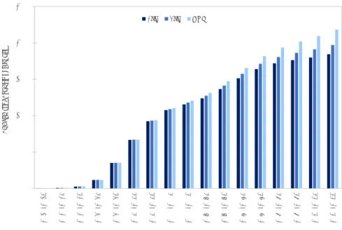
Let us first see how our main results change when we use regionally disaggregated population dynamics. Figure C.13 reproduces the aggregate climate change-related deaths and life-years lost per annum due to climate change. They can therefore be compared to Figures 4 and 6.

0 50 100 150 200 250 300 350 400 201 5-201 9 202 0-202 4 202 5-202 9 203 0-203 4 203 5-203 9 20 40 -20 44 204 5-204 9 205 0-205 4 205 5-205 9 20 60 -20 64 206 5-206 9 207 0-207 4 207 5-207 9 208 0-208 4 208 5-208 9 209 0-209 4 20 95 -20 99 de aths (tho us and s pe r ye ar) 2°C 3°C BAU

(a) Climate change-related deaths per an-num 0 2 4 6 8 10 2015-2019 2020-2024 2025-2029 2030-2034 2035-2039 2040-2044 2045-2049 2050-2054 2055-2059 2060-2064 2065-2069 2070-2074 2075-2079 2080-2084 2085-2089 2090-2094 2095-2099 lif e-ye ar s lo st (m il li ons pe r ye ar ) 2°C 3°C BAU

(b) Life-years lost per annum due to climate change

Figure C.13: Climate change-related deaths and life-years lost per annum due to climate change using a regionally-disaggregated model

It appears that our main results are robust to the regional disaggregation of population dynamics. Although there are small di↵erences in the numbers, the general trends and conclusions still hold.

We can then look at how these aggregate figures are distributed across regions. To do so, we will focus on numbers of life-years lost per annum, which is probably the most welfare relevant metric. Table C.2 show these results for the 2 C (in blue) and the BAU (in red) scenarios.

Table C.2 highlights the di↵erent regional patterns and absolute values of number of life-years lost due to climate change. In terms of patterns, Asia is projected to experience a decrease in life-years lost both in the 2 C and in the

10_{RICE was developed by William Nordhaus (see Nordhaus, 2010, for a presentation of the} model).

Africa Asia Europe N. America L. America Oceania 2015-2019 4.866 3.749 0.041 0.019 0.154 0.002 4.866 3.749 0.041 0.019 0.154 0.002 2020-2024 5.096 3.481 0.047 0.023 0.145 0.002 5.130 3.505 0.048 0.024 0.146 0.002 2025-2029 5.269 3.213 0.054 0.029 0.137 0.002 5.405 3.296 0.055 0.029 0.141 0.002 2030-2034 5.348 2.976 0.061 0.034 0.131 0.003 5.641 3.139 0.065 0.036 0.138 0.003 2035-2039 5.344 2.788 0.068 0.039 0.126 0.003 5.834 3.044 0.074 0.042 0.138 0.003 2040-2044 5.268 2.616 0.074 0.043 0.124 0.003 5.979 2.970 0.084 0.049 0.141 0.004 2045-2049 5.139 2.450 0.079 0.046 0.123 0.003 6.082 2.900 0.094 0.054 0.146 0.004 2050-2054 4.965 2.298 0.084 0.047 0.124 0.004 6.138 2.842 0.103 0.058 0.153 0.004 2055-2059 4.774 2.161 0.087 0.049 0.126 0.004 6.174 2.795 0.112 0.064 0.163 0.005 2060-2064 4.575 2.054 0.087 0.051 0.127 0.004 6.193 2.782 0.118 0.069 0.173 0.005 2065-2069 4.371 1.957 0.086 0.053 0.130 0.004 6.200 2.777 0.122 0.076 0.184 0.006 2070-2074 4.165 1.867 0.084 0.055 0.131 0.004 6.199 2.780 0.125 0.082 0.195 0.007 2075-2079 3.965 1.766 0.082 0.057 0.131 0.005 6.205 2.764 0.128 0.089 0.206 0.007 2080-2084 3.779 1.663 0.081 0.057 0.131 0.005 6.224 2.741 0.133 0.093 0.216 0.008 2085-2089 3.621 1.570 0.080 0.057 0.130 0.005 6.281 2.725 0.140 0.098 0.226 0.008 2090-2094 3.485 1.493 0.081 0.057 0.128 0.005 6.359 2.726 0.147 0.104 0.233 0.009 2095-2099 3.367 1.435 0.080 0.057 0.126 0.005 6.449 2.751 0.154 0.109 0.241 0.009

Table C.2: Decomposition of the number of life-years lost due to climate change in two scenarios (2 C, BAU)

BAU scenarios. On the contrary, Europe, North America and Oceania are pro-jected to experience an decrease in life-years lost in the two scenarios. Africa and Latin America have less clear patterns, but in the whole they are projected to experience a decrease in life-years due to climate change in the 2 C scenario, but an increase in the BAU scenario.

In terms of the absolute values, it clearly appears that Africa and Asia bear the brunt of the overall impact. In the BAU scenario, Africa accounts for 55% of