HAL Id: hal-01369525
https://hal.archives-ouvertes.fr/hal-01369525
Submitted on 28 Apr 2021HAL is a multi-disciplinary open access archive for the deposit and dissemination of sci-entific research documents, whether they are pub-lished or not. The documents may come from teaching and research institutions in France or abroad, or from public or private research centers.
L’archive ouverte pluridisciplinaire HAL, est destinée au dépôt et à la diffusion de documents scientifiques de niveau recherche, publiés ou non, émanant des établissements d’enseignement et de recherche français ou étrangers, des laboratoires publics ou privés.
Finite element modelling of 1D steel components in
reinforced and prestressed concrete structures
Antoine Llau, Ludovic Jason, Frédéric Dufour, Julien Baroth
To cite this version:
Antoine Llau, Ludovic Jason, Frédéric Dufour, Julien Baroth. Finite element modelling of 1D steel components in reinforced and prestressed concrete structures. Engineering Structures, Elsevier, 2016, 127, pp.769-783. �10.1016/j.engstruct.2016.09.023�. �hal-01369525�
1
Finite Element modelling of 1D steel components in
reinforced and prestressed concrete structures.
Antoine Llau a,b,c*, Ludovic Jason a,b, Frédéric Dufour c,d, Julien Baroth c,d a SEMT, CEA DEN, Université Paris Saclay, 91191 Gif sur Yvette Cedex, France
b IMSIA, CEA, CNRS, EDF, ENSTA Paristech, Université Paris Saclay, 91762 Palaiseau Cedex, France c Univ. Grenoble-Alpes, 3SR, 38041 Grenoble, France
d CNRS, 3SR, 38041 Grenoble, France
* Corresponding author: SEMT, CEA DEN, Université Paris Saclay, 91191 Gif sur Yvette Cedex, France
antoine.llau@3sr-grenoble.fr, +33 (0)169088747
Abstract
This paper introduces a new approach for FE modelling of 1D steel inclusions within a 3D concrete domain. Reinforcements modelled with 1D meshes, when included in 3D domains, are indeed responsible for pathological effects like stress concentration at the local scale. The alternative solution of an explicit 3D mesh of the steel elements requires a large amount of work, and a relatively fine conform mesh (and therefore, additional computation cost). It is thus hardly applicable to large-scale structures. The approach proposed in this contribution, called “1D-3D”, generates an equivalent volume from a 1D mesh of the reinforcements. Associated stresses and stiffnesses, which can be condensed on the boundaries of the newly created volume, are then applied to concrete 3D elements using kinematic relations. This approach is validated on two representative cases of civil engineering applications, including active and passive steel reinforcements. It provides results similar to an explicit 3D approach, without its meshing complexity. It thus combines the advantages of 1D and 3D approaches in a single modelling.
Keywords
2
1 Introduction
In civil engineering, structures are usually built using reinforced or prestressed concrete. The role of passive or active (tendons) reinforcement is to delay the formation of cracks [1–3]. Many FE constitutive laws are able to represent the mechanical behavior of plain concrete at various scales with great accuracy [4–6]. They also ensure numerical stability if advanced numerical methods are used [7– 9]. However, the way to model the steel components embedded in the concrete is still an issue. Three main approaches are generally chosen to represent 1D steel members in 3D concrete structures when large-scale structures are considered [10]: the “classical” 1D approach [11], the homogenized 2D approach [12], and the richer “full 3D” approach [13,14].
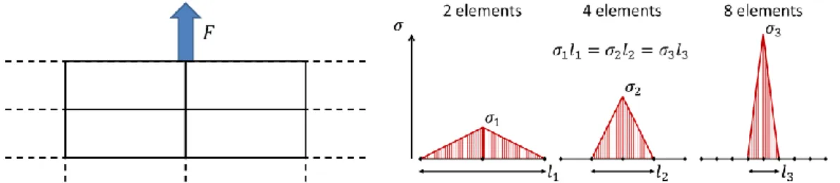
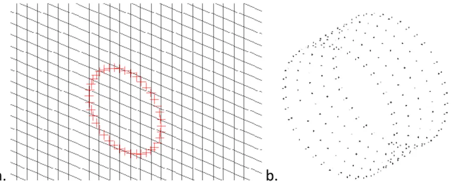
The 1D approach (Figure 1a) is by far the most widely used in literature to represent these steel members [10,15–17]. It is simple to apply on large and complex structures as it does not require any mesh constraints. The reinforcement is represented using either beam or truss finite elements [18]. From a geometrical point of view, its diameter is neglected compared to its own length and to the concrete matrix finite element’s size. From a mechanical point of view, a superimposition of the materials is supposed in terms of local stiffness, and the cross section is used solely to compute stress and stiffness values (and not their repartition). Therefore, a singularity is created. The steel and concrete are related using either a corresponding mesh, kinematical relations or specific rebar-concrete bond models [19–21]. This strategy is easy to use and able to reproduce the structural behavior. However, at the local scale, it fails to reproduce certain specific configurations, involving for instance transversal effects [10]. Moreover, it is often associated to a stress concentration phenomenon, especially when active reinforcements are considered (Figure 2). This leads to a pathological mesh dependency and nonphysical results: in particular, stress singularities will yield a very early damage initiation [22].
a. b.
Figure 1 : Resulting mesh of a reinforced concrete structure using either 1D (a) or 3D (b) approaches for the steel reinforcement.
3
Figure 2 : Illustration of the stress concentration effect with a 2D material problem for a given nodal force. An alternative approach considers a homogenized model of the reinforcements, which uses 2D plate or shell elements. From a geometrical point of view, the regular pattern of rebars is considered as a homogeneous plate embedded in the concrete. The cross-section is once again only used to compute the stresses, and the materials are superimposed. This approach is easy to use on large-scale reinforced concrete problems, and can reproduce the structural behavior. It also avoids creating geometrical singularities and does not suffer from numerical instability at the local scale. However a homogenized approach is unable to represent the local effects associated to heterogeneous reinforcements (such as stirrups). It is also limited to regular patterns of reinforcements, and not fully adapted to the representation of prestressing tendons for instance.
Another approach considers a full 3D steel volume inside the concrete domain (Figure 1b). It is much richer (representation of the kinematics) but the counterpart is a mesh complexity and a higher computational cost. At the steel-concrete interface, the meshes are indeed coincident to avoid superimposition. This solution presents several advantages, mainly a richer representation of the mechanical behavior at the local scale and a stability of the results regarding the mesh. However, although it may be automated up to a certain limit, the necessary effort on the mesh is hardly compatible with industrial computations (especially for a high density or complex geometry of the reinforcements). This is the reason why this approach is rather rare in the literature, except when an explicit 3D representation interface is needed (steel-concrete bond models for example [13,21,23,24], or models including corrosion [25]).
Other approaches have also been recently developed, such as [26] with a global-local coupling. In the case of problems solved by extended finite elements (X-FEM) for instance, modelling strategies based on level-sets have also been developed to represent these inclusions [27,28]. However, these strategies both require a relatively fine mesh around the reinforcements, which makes them hardly applicable on large-scale structures.
Regarding the limits of the existing approaches (stress concentration, meshing difficulty, and capacity to be applied to either fine or coarse meshes but not both…) a new approach is proposed in this contribution. Called 1D-3D approach (1D reinforcements - 3D FE domain), it should combine the advantages of both 1D and 3D approaches. In particular, it aims at providing structural quantities of
4
interest for coarse meshes (as 1D models), and structural and local quantities of interest for fine meshes (as 3D models) without stress concentration. It should be able to characterize the mechanical effect of reinforcements in nonlinear solid mechanics problems involving various types of behavior laws for the reinforcement and matrix and solved by the finite element method.
In this contribution, the proposed approach is first described. Then, an academic case (a single active tendon in a curved concrete volume [11]) is presented to validate the approach. A comparison with 1D and 3D approaches is especially proposed. Finally, a Representative Structural Volume of containment buildings [29] is considered to underline the interest of the proposed approach on a more complex structure.
2
Presentation of the “1D-3D” approach
The 1D-3D approach aims at combining the advantages of both 1D and full 3D approaches. The main objective is especially to keep low the required effort to produce the mesh (1D approach) and to obtain representative local results, especially when the mesh is fine (3D approach). Moreover, a particular attention will be paid to the possibility to reuse existing 1D meshes to improve former computations. The proposed “1D-3D” approach works in four steps:
- generation of the equivalent volume of the reinforcement. - computation of the equivalent forces.
- condensation of the 3D equivalent volume on its boundary. - introduction of relations at the steel-concrete interface.
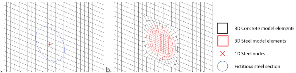
2.1 Generation of the equivalent volume of the reinforcement
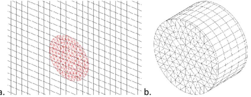
The 1D-3D approach relies on a 1D mesh of the steel components. A 3D equivalent volume is then generated using the 1D mesh as a directrix. The cross section is created using triangle elements, with a concentrical discs iterative algorithm (Figure 3). This meshing strategy has been chosen as it generates a very regular mesh in the (expected) case of a circular cross-section; however it is not required for our approach and could be replaced by other techniques, such as Delaunay triangulation. The equivalent volume is finally obtained with prismatic elements, by projection of the circular cross sections along the directrix (Figure 4). Concrete mesh is not modified. The mesh of the newly created cross section is proposed to be twice as fine as the concrete mesh. This allows to include steel nodes in all concrete elements around the heterogeneity. This is necessary to ensure a good repartition of the steel stiffness and nodal forces in the neighboring concrete elements, and to avoid local singularities. Along the axis of the bar, the density of the mesh is proposed to be the same as the 1D mesh.
5
Figure 3: Construction of the circular cross section of the 1D-3D mesh: 5 steps (red: goal cross section).
a. b.
Figure 4 : Mesh of the steel cross section inside concrete (a) and mesh of the steel bar (b) with the 1D-3D approach.
2.2 Computation of the equivalent forces
In some cases (prestressed tendons, temperature loading…), loading may be applied directly on the inclusion. In those situations, the proposed 1D-3D approach requires transposing the stress state computed on the 1D tendon (denoted 𝜎1𝐷) to a stress state on the equivalent 1D-3D tendon
(denoted 𝜎1𝐷3𝐷). The 1D stress state is first converted into nodal forces: 𝐹𝑖= 𝑆 ∫
𝑑𝜎1𝐷
𝑑𝑙 𝑑𝑙
𝐿𝑖
(1) where 𝐹𝑖 are the nodal forces at node 𝑖, 𝑆 the cross section of the heterogeneity and 𝑙 the abscissa
along the 1D inclusion, integrated along a relevant subdomain of length 𝐿𝑖 (depending of the FE
interpolation functions). These nodal forces are then applied on the 1D-3D bar, to obtain the stress field in the equivalent volume, such that:
𝐹𝑖= ∫ ∇𝜎1𝐷3𝐷𝑑𝑉 𝑉𝑖
(2) where ∇ stands for the divergence, 𝑉 is the volume of the bar and 𝑉𝑖 is the volume of the relevant
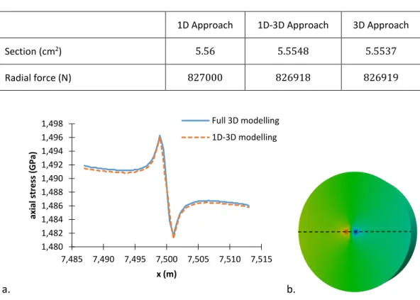
subdomain (depending on the FE geometry and interpolation functions). As an illustration, Figure 5 presents the (initial) stress distribution simulated on a curved steel tendon before the application of the prestress to the concrete. It compares the full 3D and the 1D-3D approaches. The stress distributions are similar in both cases. To supplement the comparison, values of the resulting radial
6
force created by the internal stresses in the tendon are compared to the force applied in the 1D case (Table 1). The relative error on the global longitudinal force is of the order of 10−4; the error on the cross-section, due to the discretization of the tendon, is of the order of 10−3. Figure 6 also presents the longitudinal stress in the tendon along the 𝑥 axis (horizontal axis of the cross-section). A slight localization appears in both approaches near the central area (along the position of the 1D tendon). The relative error in longitudinal stress between both models remains lower than 0.1 %.
a. b.
Figure 5 : Axial stress distributions in a curved prestressed tendon: 1D-3D approach (a), full 3D approach (b). Table 1: Resulting radial force on the tendon cross-section.
1D Approach 1D-3D Approach 3D Approach Section (cm2) 5.56 5.5548 5.5537
Radial force (N) 827000 826918 826919
a. b.
Figure 6: Longitudinal stress in the tendon after computation of the equivalent forces (a), along a line (b). 2.3 Condensation of the 3D equivalent volume
Compared to the 1D modelling, the creation of the equivalent steel volume in the 1D-3D approach entails a larger number of nodes and elements. The number of these additional degrees of freedom
1,480 1,482 1,484 1,486 1,488 1,490 1,492 1,494 1,496 1,498 7,485 7,490 7,495 7,500 7,505 7,510 7,515 ax ial str e ss (GP a) x (m) Full 3D modelling 1D-3D modelling
7
may be low compared to the total number of degrees of freedom (dofs) if large concrete structures with low numbers of inclusions are considered. But the additional computational cost may become a key issue when large-scale heavily reinforced structures (typically in civil engineering applications) are studied.
a. b.
Figure 7 : 1D-3D condensation nodes where the stiffness and forces are applied: side view (a) and 3D view (b). Therefore, an approach is proposed to reduce the number of dofs. It is similar to the adaptive condensation technique presented in [30]. It uses a static condensation technique [31] to replace the equivalent volume by its consequences in terms of stiffness and loading on the boundary of the volume of the heterogeneity (Figure 7). This choice allows to reduce the 3D equivalent volume to a 2D surface. The equation of static writes for the steel volume:
𝐾𝑈 = 𝐹 (3)
where 𝐾 is the stiffness matrix, 𝑈 the nodal displacement vector, and 𝐹 the vector of equivalent external nodal forces. The decomposition between the boundary area Ω𝑏, which represents the
boundary of the steel volume, and the eliminated area Ω𝑒, which represents its inner volume, writes: [𝐾𝐾𝑒,𝑒 𝐾𝑒,𝑏 𝑏,𝑒 𝐾𝑏,𝑏] [ 𝑈𝑒 𝑈𝑏] = [ 𝐹𝑒 𝐹𝑏] (4) The subdomain Ω𝑒can be eliminated to obtain the reduced system [31]:
𝐾̂𝑈𝑏= 𝐹̂ (5)
with the reduced stiffness matrix and reduced forces vector:
𝐾̂ = 𝐾𝑏,𝑏− 𝐾𝑏,𝑒𝐾𝑒,𝑒−1𝐾𝑒,𝑏
𝐹̂ = 𝐹𝑏− 𝐾𝑏,𝑒𝐾𝑒,𝑒−1𝐹𝑒
(6)
The full equivalent 1D-3D volume can then be replaced by a reduced stiffness matrix and a force vector applied on its boundary. It is to be noted that, with this approach, the mechanical state of the inner volume (strain, internal displacement, stresses…) can still be obtained by a simple linear resolution of the condensed subproblem (also called de-condensation [30]):
8
𝑈𝑒= 𝐾𝑒,𝑒−1(𝐹𝑒− 𝐾𝑒,𝑏𝑈𝑏) (7) As an illustration, for a straight bar of diameter 2𝑅 and length 𝐿, meshed with finite elements of length 𝑙, the approximate number of nodes 𝑛𝑓 in the full equivalent volume writes:
𝑛𝑓=
2𝜋𝑅2𝐿
√3 𝑙3
(8) The number of nodes 𝑛𝑐 in the condensation area writes:
𝑛𝑐 = 2𝜋𝑅𝐿 𝑙2 (9) Then: 𝑛𝑓/𝑛𝑐 = 𝑅 √3 𝑙 (10) For example, with 𝐿 = 2 m, 𝑅 = 84 mm, and 𝑙 = 5 mm, the ratio 𝑛𝑓/𝑛𝑐 is close to 10. It may be
observed that the stiffness matrix obtained from condensation is smaller than the base matrix. However it is also denser, which may negatively impact computational performance, depending on the type of linear solver. To improve this aspect, the condensed matrix may be approximated by removing low terms or using limited-rank approximation methods such as truncated SVD [32,33]. In the proposed approach, condensation may or may not improve computational performance, depending on the chosen case (and particularly, on the geometry of the inclusions). That is why this step remains facultative. Moreover, the condensation requires the inclusion to remain linear-elastic, which is generally the case for prestressed tendons in concrete for example. If not, the methodology can be used, without condensation on the inclusion boundary.
2.4 Inclusion-domain interface
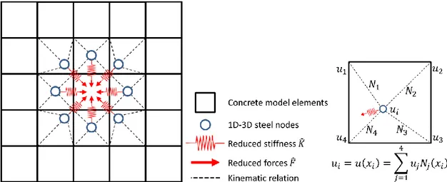
For the bond between the inclusion and the domain, the nodes at the interface (Ω𝑏) need to be related
to the concrete ones, in order to ensure the conformity of the displacement fields and transmit the stiffness and forces coming from the 1D-3D inclusion. Various methods have been proposed in the literature that could match these objectives [34,35]. The Multi-Point Constraint is the first and simplest method available. It ensures a strong coupling between the subdomains; however it suffers from sensitivity to the choice of slave/master nodes [36]. To avoid this problem, two-pass approaches have been developed, that eliminate the master and slave choice. However they tend to suffer from severe mesh locking [37]. Considering dual approaches, Lagrange multiplier fields can be used to enforce the weak compatibility of the interfaces. The mortar method is one of the most common [38]. It avoids the surface locking and, with further developments, is independent of the mesh size [39]. Nevertheless, it tends to generate stress oscillations. Arlequin method [40], developed in particular for overlapping
9
domains does not generally suffer pathological stress oscillations. However it requires additional degrees of freedom, and the definition of overlap areas and transition functions. Considering primal approaches, discontinuous Galerkin framework may be the most widely used [41], as it is stable and relatively simple to implement. However, it requires the definition of a mesh-dependent penalty factor (as in Nitsche’s method [42]) and tends to have a high computational cost. In the Interface Element Method [43], additional elements are created using the nodes of the interface. This allows to include a behavior law for the interface, but requires modifying the shape functions on the interface elements. In our approach, given that the 1D-3D mesh has, by design, the same size as the concrete mesh and that both are overlapping, and since the reinforcement is much stiffer than the concrete, the reinforcement interface nodes Ω𝑏 are related to concrete by MPC-type kinematic relations on
displacements, enforced using the double Lagrange multipliers method (Figure 7-8) [44]. The displacement 𝑢𝑖 of the (slave) reinforcement boundary node 𝑖 is such that:
𝑢𝑖= ∑ 𝛼𝑗𝑢𝑗 𝑗
(11) where 𝑢𝑗 are the displacements of the (master) nodes 𝑗 of the 3D concrete finite element in which 𝑖 is
located, and 𝛼𝑗 are linear combination coefficients defined by a linear interpolation of displacements
𝑢𝑗 at the position of the node 𝑖 (Figure 8).
It is to be noted that this approach is similar to the perfect bond relation usually considered for 1D heterogeneities (in the case of non-corresponding meshes). However, for RC applications, this relation could be improved to include a more representative steel-concrete bond behavior (such as [20,21,45]), or to take into account accurately the conformity of displacement fields between steel and concrete in the case of quadratic elements.
Figure 8: Scheme of the condensed 1D-3D approach applied on a RC structure, and zoom on one concrete finite element with a steel node.
10
As it is the case with the classical 1D modelling, the effect of superimposition of steel and concrete (additional stiffness) is neglected. At the fine scale of full 3D modelling of reinforcements, this overlapping may seem a rather coarse approximation. Nevertheless, the influence of this overlapping should be investigated. On the tested configurations, it has not been found significant. In the case in which it would be, other strategies would be possible (removing the concrete elements embedded in the steel for instance).
As a conclusion, the developed method can be used automatically from existing 1D meshes. It does not suppose any further meshing effort. The only additional cost, compared to a 1D representation, is a computational one due to the additional kinematical relations and the cost of the condensation of the inner equivalent volume (if done). This slight increase of the computational cost is expected to produce more accurate and stable local stress field as it will be analyzed in the following section.
3 Validation on a curved prestressed volume
3.1 Presentation
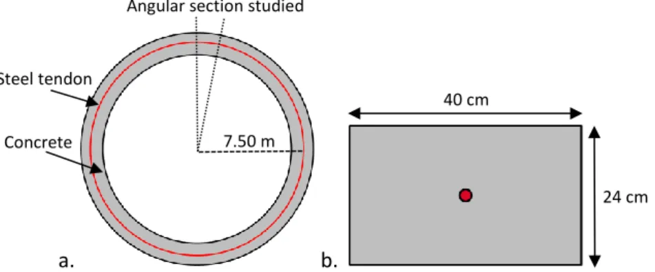
The proposed test case aims at validating the developed approach through a comparison with the 3D “reference” solution. It consists in a curved concrete volume with a single horizontal tendon. Dimensions have been chosen to match the scale of the containment mock-up VeRCORS [46,47].
a. b.
Figure 9 : Geometry of the curved prestressed concrete volume. a: Top view. b: Section.
Figure 9 presents the geometry: the horizontal tendon has the same curvature radius (7.50 m) as the center of the concrete volume. The cross section of the tendon is 5.56 cm2 (diameter 𝜙 = 26.6 mm). The concrete is meshed with cubic elements, and follows at first an elastic behavior law (𝐸 = 30 GPa, 𝜈 = 0.2). Boundary conditions enforce the rotational invariance of the problem: normal displacements are prohibited on the front, back, top and bottom faces of Figure 9b. The only applied loading is the prestress (1.5 GPa), which entails a compressive stress in concrete equal to around 8 MPa. In this simplified structure, no loss of prestress is considered. The simulations are performed with the FE code Cast3M [44].
40 cm
24 cm 7.50 m
Steel tendon Concrete
11
When prestress is applied, the tendon is responsible for both orthoradial and radial nodal forces (due to curvature) [48]. This latter loading puts the concrete FE located directly inside the curvature of the cable in radial compression, and those directly outside the curvature in radial tension.
3.2 Results
3.2.1 Structural comparison
To position the proposed approach among the existing solutions, results are compared to 1D and full 3D approaches. In every case, the concrete mesh is almost the same and only differs in the tendon area for the full 3D tendon modelling (to match the steel-concrete interface, Figure 10). Figure 11 presents the equivalent strain distributions at the end of the application of the prestress. The equivalent strain (using Mazars’ definition commonly chosen for concrete cracking modelling in the framework of damage mechanics [5]), which writes:
𝜀̅ = √⟨𝜀1⟩+2 + ⟨𝜀2⟩+2+ ⟨𝜀3⟩+2
(12)
where 𝜀1, 𝜀2, 𝜀3 are the principal values of strain, and ⟨𝜀1⟩+, ⟨𝜀2⟩+, ⟨𝜀3⟩+ the positive parts of each of
these principal values. The distributions of the equivalent strain are similar between the three modellings. The equivalent strain is especially larger in the zone directly outside the curvature of the tendon and lower in the zone directly inside (left side on the figure). As expected, this local effect is due to the curvature [48] of the tendon and is well captured in all cases.
a. b. c.
Figure 10: Meshes of the tendon area: 1D modelling (a), 1D-3D modelling (b), full 3D modelling (c).
a. b. c.
Figure 11: Equivalent strain distributions on the curved concrete volume: 1D modelling (a), 1D-3D modelling (b) and 3D modelling (c). In sid e Outsid e
12
Table 2: Structural prestress effect on concrete (radial displacement are observed on the interior lower point).
1D Approach 1D-3D Approach 3D Approach Elastic energy in concrete (J) 76.08 76.56 76.65 Radial displacement (mm) −2.164 −2.171 −2.179
Overall, the structural prestressing compressive effect is well reproduced: the values of the elastic energy which is stored in the concrete volume and of the radial displacements are similar for the three modellings (Table 2). A stability of the concrete elastic energy with the mesh is also noticed: in every case the variation is lower than 2 % with meshes ranging from 80 mm to 1.9 mm (Figure 12). It is to be noticed that the slight variation in the energy observed with 1D-3D and 3D approaches may be due to the discretization of the tendon which is modified when the mesh changes. It is not the case with the 1D modelling. That is why a “perfect” stability is obtained in this case.
Figure 12: Elastic energy stored in the concrete volume depending on element size.
a. b.
Figure 13: Longitudinal stress in the curved tendon after prestressing (a) along a line (b).
75,8 76,0 76,2 76,4 76,6 76,8 77,0 77,2 77,4 77,6 1 10 100 1000 10000 El asti c e n e rg y (J) Element section (mm2) 1D Approach 3D Approach 1D-3D Approach In cl u si o n s ec ti o n 1,490 1,492 1,494 1,496 1,498 1,500 1,502 1,504 1,506 7,485 7,490 7,495 7,500 7,505 7,510 7,515 ax ial str e ss (GP a) x (m) Full 3D modelling 1D-3D modelling
13
Figure 13 presents the longitudinal stress in the tendon along the 𝑥 axis (horizontal axis of the cross-section) for the full 3D and 1D-3D modellings (for a 2 mm mesh). The evolutions follow the same tendency, with a slight decrease as 𝑥 increases (outside of the curvature). The difference between both evolutions (maximum relative error equal to 0.453 %) can be explained by the overestimation of the local stiffness (superimposition of steel and concrete) in the 1D-3D approach.
a. b. c. 7,0E-5 8,0E-5 9,0E-5 1,0E-4 1,1E-4 1,2E-4 1,3E-4 7,30 7,40 7,50 7,60 7,70 e q u iv al e n t str ai n x (m) 1D-3D modelling 3D modelling 1D modelling 7,0E-5 8,0E-5 9,0E-5 1,0E-4 1,1E-4 1,2E-4 1,3E-4 7,30 7,40 7,50 7,60 7,70 e q u iv al e n t str ai n x (m) 1D-3D modelling 3D modelling 1D modelling 7,0E-5 8,0E-5 9,0E-5 1,0E-4 1,1E-4 1,2E-4 1,3E-4 7,30 7,40 7,50 7,60 7,70 e q u iv al e n t str ai n x (m) 1D-3D modelling 3D modelling 1D modelling
14 d.
e. f.
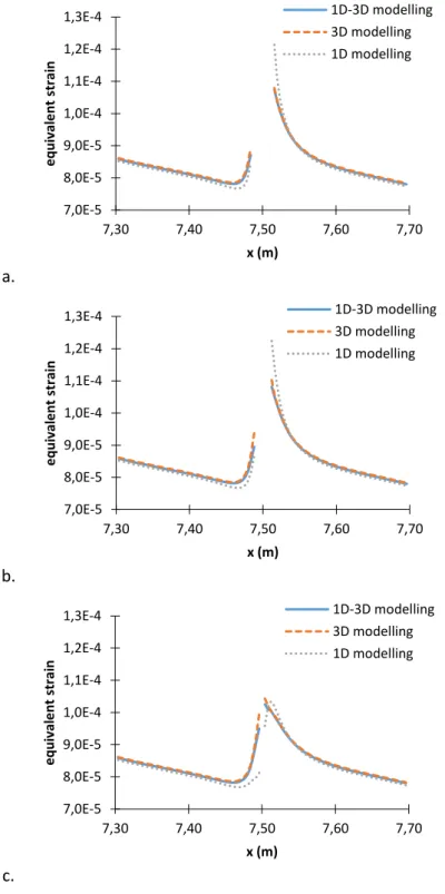
Figure 14: Values of the equivalent strain in the concrete on horizontal lines (f) of the cross-section (a: line 0, b: line 1, c: line 2, d: error map on the three lines with the 1D-3D approach, e: error map on the three
lines with the 1D approach (f). The error estimation requires a projection in this case).
Figure 14 presents the values of the equivalent strain along three horizontal lines located in a cross-section of the concrete volume, and the relative error made by the 1D and 1D-3D approaches compared to the full 3D approach. It is to be noted that since the meshes are not identical, a projection was required to compute the error, which may induce additional error. With the 1D-3D approach, the error is low far away from the tendon; in the neighborhood of the tendon, the error rises up to 5 % in several points, which remains acceptable considering the heterogeneity. As a comparison, the error of the 1D modelling reaches more than 15 % near the reinforcement.
3.2.2 Local comparison – stress concentration
The three approaches capture correctly the structural compressive and curvature effects due to the tendon. However, results at the local scale may vary significantly depending on mesh size when using 1D representations. Figure 15 presents the distribution of the radial stress in the concrete volume after the prestress, for two different mesh sizes, using a 1D representation. In the concrete FEs directly
0,00 0,01 0,02 0,03 0,04 0,05 7,30 7,40 7,50 7,60 7,70 1D -3D ap p ro ac h e rr o r x (m) line 0 line 1 line 2 0,00 0,05 0,10 0,15 0,20 7,30 7,40 7,50 7,60 7,70 1D ap p ro ac h e rr o r x (m) line 0 line 1 line 2 line 2 line 1 line 0
15
inside and outside the tendon’s curvature, significant low and high stress values are noticed: they are both concentrated on the FEs adjacent to the 1D tendon. This is locally non representative of the physical phenomena: the geometrical (and thus mechanical) singularity entails a stress localization on one FE whatever its size.
a. b.
Figure 15 : Distributions of radial stress on the curved concrete volume with a 1D modelled tendon: 16 mm mesh (a) and 3.8 mm mesh (b).
This localization effect, that has been qualitatively underlined, can also be theoretically investigated [22,49]. We summarize in the following some theoretical results from [49], applied to the problem of a 1D reinforcement in a 3D structure. To simplify the theoretical study, the simplified case of a conform mesh with a 1D inclusion is considered. In this case, the nodal forces due to the 1D tendon are applied on one node irrespectively of the FE size.
Figure 16: Illustration of element contributions to nodal force
The nodal force applied on a concrete node 𝑖 writes as a sum of the contributions of the adjacent concrete finite elements (Figure 16, for 1 ≤ 𝑒 ≤ 4):
𝐹𝑖= ∑ 𝐹𝑖𝑒 𝑒
(13)
where 𝐹𝑖 is the nodal force at node 𝑖, and 𝐹𝑖𝑒 the contribution of finite element 𝑒 to 𝐹𝑖. Each finite
element contribution 𝐹𝑖𝑒 writes:
𝐹𝑖𝑒= ∫ (𝐵𝑖𝑒)𝑡𝜎𝑒𝑑Ω Ωe (14) In sid e Outsid e
16
where 𝐵𝑖𝑒 is the derivative matrix of the interpolation functions of node 𝑖 in the finite element 𝑒, 𝜎𝑒
the stress value, Ω𝑒 the support of the finite element 𝑒. In practical cases, the integral is approximated
using for instance Gauss quadrature methods, giving:
𝐹𝑖𝑒= ∑ 𝜔𝑔𝐵𝑖 𝑔 𝜎𝑔 𝑁𝐺(𝑒) 𝑔=1 (15)
where 𝜔𝑔 are the quadrature weights, 𝐵𝑖𝑔 and 𝜎𝑔 are respectively the values of 𝐵𝑖 and 𝜎at the 𝑁𝐺
Gauss points of the FE 𝑒. When the mesh is refined (typical FE dimension equal to 𝑙), the node 𝑖 belongs to smaller finite elements. The interpolating functions are modified, and follow an evolution such that 𝐵𝑖𝑔 ∼ 𝑙−1. The integral term also varies, as the support Ω𝑒 of the shape functions shrinks
depending on the dimension 𝑑 of the space; its measure follows the relation 𝜇(𝛺𝑒) ∼ 𝑙𝑑. This
translates to the quadrature weights as:
𝜔𝑔≃ 𝜔 0 𝑔 . (𝑙 𝑙0 ) 𝑑 (16) where 𝜔0 𝑔
and 𝑙0 are reference values for 𝜔𝑔 and 𝑙. Therefore, if the contribution of the FE 𝑒 to the
nodal force 𝐹𝑖 remains constant (which is the case in the studied problem), it appears that: 𝜎𝑒≃ 𝜎0. (
𝑙0
𝑙)
(𝑑−1)
(17) where 𝜎0 is a reference value for 𝜎𝑒. Therefore, when the mesh is refined, the stress values in the
concrete FEs adjacent to the steel node depend directly on the mesh size.
As an illustration, the radial stress at the singularity observed in Figure 15 is roughly 4 times higher in the 𝑙 = 3.8 mm mesh than with the 𝑙0= 16 mm mesh (for a 𝑑 = 2 dimensional problem). Hence,
the 1D approach is totally unable to reproduce the local stress state due to the tendon curvature. This nonphysical effect is avoided by the repartition of stiffnesses and forces in several elements using a 1D-3D modelling (Figure 17).
a. b.
Figure 17: Distributions of radial stress on the curved concrete volume with a 1D-3D modelled tendon: 16 mm mesh (a) and 3.8 mm mesh (b).
17
As a confirmation, Figure 18 presents the evolution of the maximum value of the equivalent strain, depending on the size of the concrete FEs. It appears that this elastic result is clearly dependent on the mesh size when a 1D modelling is considered, due to pathological stress concentration. This exponential growth of the strain with the mesh size prevents from obtaining any precise local information, especially around the tendon. Figure 18 also illustrates the influence of the position of the steel nodes in the concrete FE when using a 1D modelling. In a first case (“element corner”), steel nodes are coincident with concrete ones (same nodes). In the second case (“element center”), steel nodes are positioned in the middle of the section of concrete FEs. It appears on Figure 18 that the local equivalent strain is not only influenced by the mesh size, but also by the position of the steel nodes inside the concrete elements. As the steel node is responsible for nodal forces inside the concrete FE, the repartition of stress differs and depends on the configuration. In particular, when steel nodes are at the center of the concrete FEs, a lower strain localization is observed, as the stress spreads through numerous elements. If steel and concrete meshes are coincident, stress concentration (and therefore, strain localization) is stronger. With the Full 3D modelling, no stress concentration is expected as the steel FEs scale in size with the concrete FEs. Therefore, the results obtained are stable toward the mesh (Figure 18).
Figure 18 : Maximum value of the equivalent strain in the concrete volume depending on element size. Figure 19 presents the same results, for the 1D, full 3D and 1D-3D approaches. This provides an indication on the validity domain of each approach.
We observe that, on the coarsest meshes (section larger than the inclusion, whose diameter is equal to 26.6 mm):
- the full 3D approach is hardly applicable, due to the need of coincident meshes at the boundary of the tendon which requires a mesh fine enough (Figure 19);
- the 1D and 1D-3D approaches provide similar and accurate values of the structural quantities of interest (Figure 12); 5 25 125 1 10 100 1000 10000 M ax imal M azar s str ai n ( 10 -5) Element section (mm2)
1D Approach / Element center 1D Approach / Element corner 3D Approach
18
- the 1D and 1D-3D approaches provide similar but not necessarily accurate values of the local quantities of interest (Figure 19), as the mesh may not be fine enough to capture local effects in the neighborhood of the tendon.
On the other hand, on the finest meshes (section smaller than the inclusion):
- the 1D approach does not converge and will tend to give nonphysical values (Figure 18); - the 1D-3D and 3D approaches provide similar and accurate values of the structural quantities
of interest (Figure 12);
- the 1D-3D and 3D approaches provide similar and numerically stable values of the local quantities of interest (Figure 19).
Figure 19 : Maximum value of equivalent strain in the concrete volume depending on element size. As a conclusion, the 1D-3D approach gives the same results as a 1D modelling when the mesh is coarse, and results similar to a full 3D approach when the mesh is refined. It is to be noted that no stress oscillations have been observed around the steel-concrete interface for the various meshes studied. For similar results on the intermediate meshes, the 3D approach requires more elements than the 1D-3D approach in order to catch the inclusion’s geometry, and may therefore require more computational effort in some cases (such as coarse meshes or high reinforcement densities).
Figure 20 presents the computational performance of the various approaches on the linear elastic simulation with different mesh sizes. The 1D approach remains the fastest in every case. On the coarse meshes, the 1D-3D approach is faster than the full 3D approach. However, the full 3D approach has a better performance on the finer meshes, due to the large number of kinematical relations added to the system to solve in the 1D-3D approach (this tendency does not take into account the additional meshing effort related to the 3D model). On this particular case, the optional condensation step seems
8,0 8,5 9,0 9,5 10,0 10,5 11,0 11,5 12,0 1 10 100 1000 10000 M ax imal M azar s str ai n ( 10 -5) Element section (mm2) 1D Approach 3D Approach 1D-3D Approach Fine meshes: 1D-3D ∼ 3D Coarse meshes: 1D ∼ 1D-3D In cl u si o n s ec ti o n
19
to degrade the computational performance, as it creates a smaller but denser stiffness matrix for the tendon. However, these conclusions are highly dependent on the case studied, and in particular on the geometry of the reinforcements.
Figure 20: Computation times for the prestressed concrete volume (linear elastic regime). 3.2.3 Consequences on the nonlinear behavior
To evaluate the ability of the proposed approach to be applied in a nonlinear simulation, in this section, a nonlinear constitutive law is now used for concrete. Mazars’ isotropic damage law is chosen to represent the concrete’s mechanical behavior [5,50]. Damage in tension 𝐷𝑇 and in compression 𝐷𝐶
thus write: 𝐷𝑇 = 1 −𝜀0(1 − 𝐴𝑇) 𝜀̅ − 𝐴𝑇exp(𝐵𝑇(𝜀0− 𝜀̅ )) (18) 𝐷𝐶 = 1 −𝜀0(1 − 𝐴𝐶) 𝜀̅ − 𝐴𝐶exp(𝐵𝐶(𝜀0− 𝜀̅ )) (19) where 𝜀0 is the damage threshold, 𝐴𝑇, 𝐵𝑇, 𝐴𝐶 and 𝐵𝑇 are parameters of the constitutive law and 𝜀̅ is
the equivalent strain (eq. (12)). The damage variable 𝐷 writes:
𝐷 = 𝛼𝑇𝐷𝑇+ 𝛼𝐶𝐷𝐶 (20) where 𝛼𝑇 and 𝛼𝐶 are functions of the strain tensor. The chosen constitutive law is combined with the
nonlocal stress-based method to avoid mesh dependency related to softening behavior laws. Therefore, in the previous equations (eq. (18)-(19)), the equivalent strain 𝜀̅ is replaced by the nonlocal equivalent strain 𝜀̃ [7]: 𝜀̃(𝑥) =∫ 𝜀̅(𝑠) 𝜙(𝑥 − 𝑠) d𝑠Ω ∫ 𝜙(𝑥 − 𝑠) d𝑠Ω (21) 0,1 1,0 10,0 100,0 3,0 6,0 12,0 24,0 C o mp u tati o n ti me ( s) Element length (mm) 1D approach 3D approach 1D-3D w/o cond. 1D-3D cond.
20
where 𝜀̃ is the nonlocal equivalent strain, 𝜀̅ the local equivalent strain, and 𝜙 is the regularization function (or weighting function). The weighting function takes into account the stress state and writes [51]: 𝜙(𝑥 − 𝑠) = exp (− ( 2 ‖𝑥 − 𝑠‖ 𝑙𝑐 𝜌(𝑥, 𝜎(𝑠)) ) 2 ) (22)
where 𝑙𝑐 is the nonlocal internal length and 𝜌 is a function of the stress state. In the case of the 1D-3D
and 1D approaches, the whole concrete domain (including the overlapping elements) is included in the regularization domain. Even if this choice may be considered as a first approximation, a study was performed (not presented for better clarity) to evaluate its effect. On this particular case, taking into account or not the whole concrete mesh in the regularization domain for the 1D-3D approach does not seem to have a significant incidence on the results in the area of interest.
a. b. c.
Figure 21 : Damage distributions at the end of the simulation with a 5 mm mesh: 1D modelling (a), 1D-3D modelling (b) and full 3D modelling (c).
a. b. c.
Figure 22 : Zoom in the tendon area on damage distribution with a 5 mm mesh: 1D (a), 1D-3D (b) and full 3D (c) representations of the tendon.
Prestress is increased up to 4.5 GPa in order to obtain significant damage values at the end of the loading. In these conditions, Figure 21 presents the damage distributions obtained at the end of the prestress for the three approaches. With the 1D modelling, damage goes up to 0.99, while with both full 3D and 1D-3D approaches, values are lower than 0.66. It appears that the distributions are similar in both 1D-3D and full 3D cases. Figure 22 presents a zoomed view of the damage distribution in the neighborhood of the tendon. Once again, damage distributions are similar even in the local zone. It is
In
sid
e
Outsid
21
to be noted that the area in which concrete and steel are superimposed with the 1D-3D modelling is damaged. However the internal variable does not spread outside the tendon volume.
These results show that the proposed approach is able to reproduce the 3D reference simulation, both for elastic and nonlinear regimes, and requires less effort for the meshing.
4 Simulation of a Representative Structural Volume
4.1 Presentation
In this section, a structural case is considered. It consists in a numerical simulation of a representative structural volume of a post-tensioned concrete building, on which a pressure resistance test has been performed [29,47]. It includes concrete, passive reinforcement and prestress tendons. This particular structure is known to be strongly dependent on the tendons at the local scale, which affect damage localization and failure mode [52]. In particular, previous numerical studies have observed a transversal inclusion effect on damage around a vertical steel tendon. This effect is not reproduced with a 1D modelling, but can be predicted with a full 3D modelling [10,53]. The aim is thus to evaluate the ability of the 1D-3D modelling approach to improve the simulation. Figure 23 presents the geometry of the structure: it consists in a curved, horizontally prestressed concrete volume on which an internal pressure is applied. A non-prestressed vertical tendon (corresponding to the transverse inclusion) is also included.
Figure 23 : Geometry and loading of the Representative Structural Volume [10].
Only one quarter of the structure is modelled, using symmetry conditions. Figure 24 presents the boundary conditions applied to the structural volume during the simulation: normal displacements are
22
blocked on three different faces of the volume. A uniform vertical displacement is also imposed on the top face. The 3D mesh (including the 3D steel elements) is presented in Figure 25. Concrete is modelled using 3D elements (Figure 25) and the passive reinforcements are represented using equivalent shell finite elements, in order to match previous work [10]. Horizontal and vertical tendons are meshed with either 1D or 3D elements (Figure 26). It is to be noted that the full 3D mesh is relatively complex and requires significant engineering work, although the structure is relatively small-scale compared to civil engineering structures.
Figure 24 : Boundary conditions and loading applied to the RSV [10].
Figure 25 : Full 3D mesh with tendons. Both vertical and horizontal tendons have a diameter 𝐷 = 84 mm. The meshes used in 1D, 1D-3D and full 3D approaches are the same. The only difference in the simulations is their material repartition (steel material at the location of steel in the 3D approach, concrete material in the other cases)
Figure 26: Concrete and steel meshes used for the 1D and full 3D representations. 1.2 m 0.9 m 1 m Vertical tendon Horizontal tendons concrete no concrete
23
The concrete is modelled, as in [10], with Mazars’ isotropic damage law [5], using the same parameters (compressive strength 𝑓𝑐 = 37.6 MPa, tensile strength 𝑓𝑡= 3.57 MPa). To avoid pathological mesh
dependency, the stress-based regularization method from [51] is included. The nonlocal internal length is equal to 𝑙𝐶0= 4 cm, in accordance with the results obtained in [10] regarding nonlocal length
dependency. Prestress is first applied through the horizontal tendons in 10 steps (and associated to a vertical compressive stress up to 1 MPa to represent the effect of a vertical prestress). The internal pressure is then applied, with a radial displacement control.
4.2 Results
4.2.1 Structural comparison
On this application, 1D, 3D and1D-3D approaches are compared on structural and local results. Figure 27 presents the pressure-radial displacement evolutions. The prestress triggers an initial negative radial displacement (compression of the volume [10]). The pressure loading follows first an elastic behavior. A nonlinear evolution is then observed with finally a decrease in the pressure for an increasing radial displacement. The three approaches give roughly the same results. At the end of the computation, the system enters a “strongly nonlinear” regime in which the convergence is difficult to reach. Moreover, at this point, the problem also reaches the limit of the quasi-static domain as the cracks spread quickly. These two reasons may explain why the solutions are not exactly the same, even if the main characteristics (limit pressure for example) are identical.
Figure 27 : Pressure-displacement evolution of the structure with different tendon modellings. 4.2.2 Local comparison
Figure 28 presents the damage distributions for radial displacements equal to 3 and 4.5 mm and with the different approaches. It appears that, except for the inside of the tendons, the distributions are nearly identical between 1D-3D and explicit 3D modellings. The particular role of the vertical tendon
0 0,2 0,4 0,6 0,8 1 1,2 1,4 1,6 -5 -3 -1 1 3 5 7 N o rmal ize d Pr e ssur e Radial displacement (mm) 1D Approach Full 3D Approach 1D-3D Approach
24
for the initiation and propagation of the damage is especially well reproduced. On the contrary, the 1D modelling does not reproduce this effect and simulates a more distributed damage in the whole volume. It may have heavy consequences, especially in the case where tightness is investigated (damage – permeability relations for example [54]). In this sense, the proposed approach clearly improves the description of the mechanical behavior at the local scale. Figure 29 presents the error map of the damage profiles for the 1D-3D modelling on the conform mesh. In a few elements, the error in damage rises up to 0.5, however, it is lower than 0.2 on most of the structure.
a.
b.
Figure 28 : Damage profiles with an adapted mesh: 1D approach, 3D approach, 1D-3D approach (a: radial displacement 3 mm, b: radial displacement 4.5 mm).
a. b.
Figure 29: Error on the damage profiles with the 1D-3D modelling on the adapted mesh (a: radial displacement 3 mm, b: radial displacement 4.5 mm).
25 4.2.3 Regular mesh
1D-3D and 3D approaches show equivalent results. Nevertheless, they have been applied on a mesh with an explicit representation of the horizontal and vertical tendons. If this explicit representation, which may require several hours of engineering work, is necessary for a full 3D modelling, it is not the case for the 1D-3D approach. This flexibility is one of the key points of the proposed approach. To illustrate this point, the same simulation is run with the 1D and 1D-3D modellings, using a regular mesh with no explicit mesh of the tendons (Figure 30). Figure 31 shows that the pressure-displacement evolutions are rather similar to the former simulation. Moreover, Figure 32 presents the damage distributions obtained for radial displacements of 3 mm and 4.5 mm using the 1D and 1D-3D modellings on the regular mesh. It appears that damage tends to initiate and localize around the vertical tendon when using the 1D-3D approach (similar to the results obtained with an explicit 3D mesh, Figure 28), but not with the 1D approach. The proposed modelling strategy is thus able to capture this structural effect, without the meshing effort related to a 3D explicit representation of the tendon.
a. b.
Figure 30 : Steel mesh for the 1D modelling (a), concrete regular mesh (b).
Figure 31 : Pressure-displacement evolution of the structure with different modellings of tendons.
0 0,2 0,4 0,6 0,8 1 1,2 1,4 1,6 -5 -3 -1 1 3 5 7 N o rmal ize d Pr e ssur e Radial displacement (mm) 1D-3D Approach / Regular mesh 1D Approach / Regular mesh Full 3D Approach
26 a.
b.
Figure 32 : Damage profiles with a regular mesh: 1D modelling vs. 1D-3D modelling (a: radial displacement 3 mm, b: radial displacement 4.5 mm).
5 Conclusions
A new approach for the modeling of steel components in concrete structures has been presented. This so-called 1D-3D approach involves the creation of an equivalent volume from a 1D discretization of the reinforcements, the computation of the stiffness and of the stress state in the equivalent steel volume, their optional condensation on the boundary of the steel domain to potentially limit the additional computational cost, and the introduction of a relation between steel and concrete by kinematical relations on the nodal displacements.
This approach is first validated on the academic case of a curved prestressed concrete volume. It avoids the stress concentration observed with 1D modelling approaches in the case of an active reinforcement, even in the elastic regime. On the second proposed application (representative structural volume), it reproduces local and structural behaviors (compared to an explicit 3D modelling of the steel components). It is especially able to capture local effects responsible for the initiation and propagation of damage that a classical 1D model fails to reproduce. This new approach thus combines the computational efficiency and ease of use of classical 1D approaches (no particular meshing effort especially) with the “quality” and rich kinematics of full 3D approaches at the local scale.
Future work will include new developments inside the proposed modelling strategy. In particular, a more representative relation for the steel-concrete bond could be considered, taking into account the sliding or loss of bond at the steel-concrete interface. Also, the approximation induced by the
27
overlapping of the steel and concrete has low impact on the presented cases, but this influence could be further studied and quantified. A wider array of loadings and applications could also be investigated, including cyclic loadings (provided appropriate behavior laws for the concrete and steel-concrete interface) or the effect of transverse reinforcements in bending beams.
Acknowledgements
The authors gratefully acknowledge the funding support from French National Research Agency through « MACENA » project (ANR-11-RSNR-012).
References
[1] R. Chaussin, Béton précontraint, Techniques de l’ingénieur. Les bétons spéciaux dans la construction. TIB223DUO (1990). http://www.techniques-ingenieur.fr/base- documentaire/construction-th3/les-betons-speciaux-dans-la-construction-42223210/beton-precontraint-c2360/.
[2] Prestressed Concrete Fifth Edition Upgrade: ACI, AASHTO, IBC 2009 Codes Version, 5 edition, Prentice Hall, Upper Saddle River, 2009.
[3] P. Bhatt, Prestressed Concrete Design to Eurocodes, 1 edition, CRC Press, London ; New York, 2011.
[4] J. Mazars, Application de la mécanique de l’endommagement au comportement non linéaire et à la rupture du béton de structure, Thesis, Université Paris VI, 1984.
[5] J. Mazars, G. Pijaudier-Cabot, Continuum Damage Theory - Application to Concrete, J. Eng. Mech. 115 (1989) 345–365. doi:10.1061/(ASCE)0733-9399(1989)115:2(345).
[6] N. Moës, T. Belytschko, Extended finite element method for cohesive crack growth, Engineering Fracture Mechanics. 69 (2002) 813–833.
[7] G. Pijaudier-Cabot, Z.P. Bažant, Nonlocal Damage Theory, J. Eng. Mech. 113 (1987) 1512–1533. doi:10.1061/(ASCE)0733-9399(1987)113:10(1512).
[8] J.H.P. de Vree, W.A.M. Brekelmans, M.A.J. van Gils, Comparison of nonlocal approaches in continuum damage mechanics, Computers & Structures. 55 (1995) 581–588. doi:10.1016/0045-7949(94)00501-S.
[9] Z. Bažant, M. Jirásek, Nonlocal Integral Formulations of Plasticity and Damage: Survey of Progress, J. Eng. Mech. 128 (2002) 1119–1149. doi:10.1061/(ASCE)0733-9399(2002)128:11(1119).
[10] L. Jason, S. Ghavamian, A. Courtois, Truss vs solid modeling of tendons in prestressed concrete structures: Consequences on mechanical capacity of a Representative Structural Volume, Engineering Structures. 32 (2010) 1779–1790. doi:10.1016/j.engstruct.2010.02.029.
[11] J.A. Figueiras, R.H.C.F. Póvoas, Modelling of prestress in non-linear analysis of concrete structures, Computers & Structures. 53 (1994) 173–187. doi:10.1016/0045-7949(94)90140-6. [12] L. Jendele, J. Červenka, On the solution of multi-point constraints – Application to FE analysis of
reinforced concrete structures, Computers & Structures. 87 (2009) 970–980. doi:10.1016/j.compstruc.2008.04.018.
[13] T.S. Phan, J.-L. Tailhan, P. Rossi, P. Bressolette, F. Mezghani, Numerical modeling of the rebar/concrete interface: case of the flat steel rebars, Mater Struct. 46 (2012) 1011–1025. doi:10.1617/s11527-012-9950-y.
28
[14] T. Mimoto, T. Sakaki, T. Mihara, I. Yoshitake, Strengthening system using post-tension tendon with an internal anchorage of concrete members, Engineering Structures. 124 (2016) 29–35. doi:10.1016/j.engstruct.2016.06.003.
[15] S. Ghavamian, I. Carol, A. Delaplace, Discussions over MECA project results, Revue Française de Génie Civil. 7 (2003) 543–581. doi:10.1080/12795119.2003.9692509.
[16] H.-T. Hu, F.-M. Lin, H.-T. Liu, Y.-F. Huang, T.-C. Pan, Constitutive modeling of reinforced concrete and prestressed concrete structures strengthened by fiber-reinforced plastics, Composite Structures. 92 (2010) 1640–1650. doi:10.1016/j.compstruct.2009.11.030.
[17] H.-T. Hu, Y.-H. Lin, Ultimate analysis of PWR prestressed concrete containment subjected to internal pressure, International Journal of Pressure Vessels and Piping. 83 (2006) 161–167. doi:10.1016/j.ijpvp.2006.02.030.
[18] A. Michou, F. Benboudjema, Y. Berthaud, G. Nahas, P. Wyniecki, V. Petit, J. Dubreuil, Cracking behavior of structures pre-stressed by bonded strands or unbonded strands TGG, in: Technical Innovation in Nuclear Civil Engineering (TINCE), Paris, France, 2013.
[19] A.O. Abdelatif, J.S. Owen, M.F.M. Hussein, Modelling the prestress transfer in pre-tensioned concrete elements, Finite Elements in Analysis and Design. 94 (2015) 47–63. doi:10.1016/j.finel.2014.09.007.
[20] C. Mang, L. Jason, L. Davenne, A new bond slip model for reinforced concrete structures. Validation by modelling a reinforced concrete tienull, Engineering Computations. (2015). doi:10.1108/EC-11-2014-0234.
[21] B. Richard, F. Ragueneau, C. Cremona, L. Adelaide, J.-L. Tailhan, A three-dimensional steel/concrete interface model including corrosion effects, Engineering Fracture Mechanics. 77 (2010) 951–973.
[22] E. Lorentz, Ill-posed boundary conditions encountered in 3D and plate finite element simulations, Finite Elements in Analysis and Design. 41 (2005) 1105–1117. doi:10.1016/j.finel.2005.01.002. [23] P. Dybeł, K. Furtak, The effect of ribbed reinforcing bars location on their bond with
high-performance concrete, Archives of Civil and Mechanical Engineering. 15 (2015) 1070–1077. doi:10.1016/j.acme.2015.03.008.
[24] L.A.M. Mendes, L.M.S.S. Castro, A new RC bond model suitable for three-dimensional cyclic analyses, Computers & Structures. 120 (2013) 47–64. doi:10.1016/j.compstruc.2013.01.007. [25] M. German, J. Pamin, FEM simulations of cracking in RC beams due to corrosion progress,
Archives of Civil and Mechanical Engineering. 15 (2015) 1160–1172. doi:10.1016/j.acme.2014.12.010.
[26] C. Oliver-Leblond, A. Delaplace, F. Ragueneau, Modelling of three-dimensional crack patterns in deep reinforced concrete structures, Engineering Structures. 83 (2015) 176–186. doi:10.1016/j.engstruct.2014.10.040.
[27] N. Moës, M. Cloirec, P. Cartraud, J.-F. Remacle, A computational approach to handle complex microstructure geometries, Computer Methods in Applied Mechanics and Engineering. 192 (2003) 3163–3177. doi:10.1016/S0045-7825(03)00346-3.
[28] N. Sukumar, D.L. Chopp, N. Moës, T. Belytschko, Modeling holes and inclusions by level sets in the extended finite-element method, Computer Methods in Applied Mechanics and Engineering. 190 (2001) 6183–6200. doi:10.1016/S0045-7825(01)00215-8.
[29] N. Herrmann, C. Niklasch, D. Kiefer, L. Gerlach, Y. Le Pape, S. Fortier, PACE 1450: An Experimental Test Setup for the Investigation of the Crack Behaviour of Prestressed Concrete Containment Walls, in: 16th International Conference on Nuclear Engineering, Orlando, Florida, USA, 2008: pp. 1–8. doi:10.1115/ICONE16-48029.
[30] A. Llau, L. Jason, F. Dufour, J. Baroth, Adaptive zooming method for the analysis of large structures with localized nonlinearities, Finite Elements in Analysis and Design. 106 (2015) 73– 84. doi:10.1016/j.finel.2015.07.011.
[31] R.J. Guyan, Reduction of stiffness and mass matrices, AIAA Journal. 3 (1965) 380–380. doi:10.2514/3.2874.
29
[32] Y.J. Ren, I. Elishakoff, New results in finite element method for stochastic structures, Computers & Structures. 67 (1998) 125–135. doi:10.1016/S0045-7949(97)00164-8.
[33] C. Tropea, A.L. Yarin, J.F. Foss, Springer Handbook of Experimental Fluid Mechanics, Springer Science & Business Media, 2007.
[34] G. Haikal, K.D. Hjelmstad, An enriched discontinuous Galerkin formulation for the coupling of non-conforming meshes, Finite Elements in Analysis and Design. 46 (2010) 496–503. doi:10.1016/j.finel.2009.12.008.
[35] L.A.G. Bitencourt Jr., O.L. Manzoli, P.G.C. Prazeres, E.A. Rodrigues, T.N. Bittencourt, A coupling technique for non-matching finite element meshes, Computer Methods in Applied Mechanics and Engineering. 290 (2015) 19–44. doi:10.1016/j.cma.2015.02.025.
[36] M. Ainsworth, Essential boundary conditions and multi-point constraints in finite element analysis, Computer Methods in Applied Mechanics and Engineering. 190 (2001) 6323–6339. doi:10.1016/S0045-7825(01)00236-5.
[37] P. Papadopoulos, R.L. Taylor, A mixed formulation for the finite element solution of contact problems, Computer Methods in Applied Mechanics and Engineering. 94 (1992) 373–389. doi:10.1016/0045-7825(92)90061-N.
[38] C. Bernardi, A new nonconforming approach to domain decomposition: the mortar element method, Nonliner Partial Differential Equations and Their Applications. (1994).
[39] B. Wohlmuth, A Mortar Finite Element Method Using Dual Spaces for the Lagrange Multiplier, SIAM J. Numer. Anal. 38 (2000) 989–1012. doi:10.1137/S0036142999350929.
[40] H.B. Dhia, G. Rateau, The Arlequin method as a flexible engineering design tool, Int. J. Numer. Meth. Engng. 62 (2005) 1442–1462. doi:10.1002/nme.1229.
[41] D. Arnold, F. Brezzi, B. Cockburn, L. Marini, Unified Analysis of Discontinuous Galerkin Methods for Elliptic Problems, SIAM J. Numer. Anal. 39 (2002) 1749–1779. doi:10.1137/S0036142901384162.
[42] J. Nitsche, Über ein Variationsprinzip zur Lösung von Dirichlet-Problemen bei Verwendung von Teilräumen, die keinen Randbedingungen unterworfen sind, Abh.Math.Semin.Univ.Hambg. 36 (2013) 9–15. doi:10.1007/BF02995904.
[43] H.-G. Kim, Interface element method (IEM) for a partitioned system with non-matching interfaces, Computer Methods in Applied Mechanics and Engineering. 191 (2002) 3165–3194. doi:10.1016/S0045-7825(02)00255-4.
[44] CEA, Description of the finite element code Cast3M, (2015). http://www-cast3m.cea.fr/.
[45] A. Casanova, L. Jason, L. Davenne, Bond slip model for the simulation of reinforced concrete structures, Engineering Structures. 39 (2012) 66–78. doi:10.1016/j.engstruct.2012.02.007. [46] B. Masson, E. Galenne, E. Oukhemanou, C. Aubry, G. Laou-Sio-Hoi, Vercors: a 1/3 scaled mockup
and an ambitious research program to better understand the different mechanisms of leakage and aging, in: Conference on Contribution of Materials Investigations and Operating Experience to LWRs’ Safety, Performance and Reliability, Avignon (France), 2014.
[47] S. Michel-Ponnelle, Description de l’essai PACE 1450 et de la maquette VeRCORS à destination du projet MACENA, Research Report - EDF R&D, 2015.
[48] S.-J. Jeon, C.-H. Chung, Axisymmetric modeling of prestressing tendons in nuclear containment
dome, Nuclear Engineering and Design. 235 (2005) 2463–2476.
doi:10.1016/j.nucengdes.2005.06.007.
[49] P. Badel, E. Lorentz, Critères de convergence en mécanique des solides, in: CSMA 2011 / 10e colloque national en calcul des structures, Giens, France, 2011. https://hal.archives-ouvertes.fr/hal-00592774/document.
[50] J. Mazars, A description of micro and macroscale damage of concrete structures, Engineering Fracture Mechanics. 25 (1986) 729–737.
[51] C. Giry, F. Dufour, J. Mazars, Stress-based nonlocal damage model, International Journal of Solids and Structures. 48 (2011) 3431–3443. doi:10.1016/j.ijsolstr.2011.08.012.
30
[52] L. Jason, S. Ghavamian, A. Courtois, Preliminary computations for a Representative Structural Volume of nuclear containment buildings, in: Proceeding of FRAMCOS 6, 2007.
[53] M. David, Approche multi-échelle du comportement mécanique des structures en béton armé - Application aux enceintes de confinement des centrales nucléaires, PhD Thesis, Ecole Polytechnique X, 2012. https://pastel.archives-ouvertes.fr/pastel-00765705/document.
[54] L. Jason, B. Masson, Comparison between continuous and localized methods to evaluate the flow rate through containment concrete structures, Nuclear Engineering and Design. 277 (2014) 146– 153. doi:10.1016/j.nucengdes.2014.06.010.