HAL Id: hal-01111720
https://hal.inria.fr/hal-01111720
Submitted on 9 Oct 2017
HAL is a multi-disciplinary open access archive for the deposit and dissemination of sci-entific research documents, whether they are pub-lished or not. The documents may come from teaching and research institutions in France or abroad, or from public or private research centers.
L’archive ouverte pluridisciplinaire HAL, est destinée au dépôt et à la diffusion de documents scientifiques de niveau recherche, publiés ou non, émanant des établissements d’enseignement et de recherche français ou étrangers, des laboratoires publics ou privés.
extreme scale computers
Fabien Rozar, Guillaume Latu, Jean Roman, Virginie Grandgirard
To cite this version:
Fabien Rozar, Guillaume Latu, Jean Roman, Virginie Grandgirard. Toward memory scalability of GYSELA code for extreme scale computers. Concurrency and Computation: Practice and Experience, Wiley, 2014, Special issue for PPAM2013 Conference, 27 (4), pp.994-1009. �10.1002/cpe.3429�. �hal-01111720�
Published online in Wiley InterScience (www.interscience.wiley.com). DOI: 10.1002/cpe
Towards Memory Scalability of G
YSELA
Code for Extreme Scale
Computers
Fabien Rozar
1 2 ∗, Guillaume Latu
1, Jean Roman
3, Virginie Grandgirard
11IRFM, CEA Cadarache, FR-13108 Saint-Paul-les-Durance 2Maison de la simulation, CEA Saclay, FR-91191 Gif sur Yvette
3Inria, Bordeaux INP, CNRS, FR-33405 Talence
SUMMARY
Gyrokinetic simulations lead to huge computational needs. Up to now, the Semi-Lagrangian code GYSELA performed large simulations using up to 65k cores. To understand more accurately the nature of plasma turbulence, finer resolutions are necessary which make GYSELAa good candidate to exploit the computational power of future Extreme scale machines. Among the Exascale challenges, the less memory per core is one of the most critical issues. This paper deals with memory management in order to reduce the memory peak and presents a general method to understand the memory behavior of an application when dealing with very large meshes. This enables us to extrapolate the behavior of GYSELAfor expected capabilities of Extreme scale machines. Copyright c 0000 John Wiley & Sons, Ltd.
Received . . .
KEY WORDS: Memory scalability, Memory footprint, Extreme scale, Plasma Physics, Gyrokinetics.
1. INTRODUCTION
The architecture of supercomputers will considerably change in the next decade. Since several years, CPU frequency does not increase anymore. Consequently the on-chip parallelism is dramatically increasing to offer more performance. Instead of doubling the clock-speed every 18-24 month, the number of cores per compute node follows the same law. These new parallel architectures are expected to exhibit different Non Uniform Memory Access (NUMA) levels and one trend of these machines will be to offer less and less memory per core. This fact has been identified as one of the Exascale challenges [SDM11] and is one of our main concerns†.
In the last decade, the simulation of turbulent fusion plasmas in Tokamak devices has involved a growing number of people coming from the applied mathematics and parallel computing fields [ ˚ACH+13]. These applications are good candidates to be part of the scientific applications that will be able to use the first generation of extreme scale computers. The GYSELAcode already
efficiently exploits supercomputing facilities [LGCDP11]. In this paper we especially focus on the memory consumption of this application. This is a critical point to simulate larger physical cases while using a constrained available memory.
∗Correspondence to: Maison de la simulation, CEA Saclay, FR-91191 Gif sur Yvette. E-mail: [email protected] †This work was partially supported by the G8-Exascale action NuFUSE contract and also by ANR GYPSI contract.
Several of the computations needed for this paper were run on the following machines: Juqueen (Germany), Turing (France), Helios (Japan). We would like to thank Julien Bigot and Chantal Passeron for fruitful discussions, valuable suggestions and the help they provided.
The goal of the work presented here is to analyze and to reduce the memory footprint of GYSELA to improve its memory scalability. We present a tool which provides a way to generate memory traces for the GYSELAapplication and a visualization of the associated memory allocations/deallocations in off-line mode. Another tool allows us to predict the memory peak depending on some input parameters. This is helpful in a production context to check whether future simulation memory needs fit into available memory. However, our final goal (not achieved yet) is to define a methodology and a versatile and portable library to assist the developer to optimize memory usage in scientific parallel applications. Preliminary version of this work has been published in [RLR14].
This article is organized as follows. The section 2 describes shortly the parallelization scheme and the memory consumption of GYSELA. The section 3 gives an overview of different approaches to handle the memory scalability issue and introduces the method we apply to decrease the memory footprint of GYSELA. In section 4, the method to decrease the memory footprint of GYSELA is described. The section 5 presents the dedicated module implemented to generate a trace file of allocation/deallocation process in GYSELA. It also illustrates the visualization and prediction tool capabilities to handle the data of the trace file. The section 6 sums up the new optimizations included step by step into the GYSELA code. The section 7 shows a study of the memory scalability of GYSELAthanks to the prediction tool, and finally, the section 8 concludes and presents future work.
2. SKETCH OF GYSELA COMPUTATION AND MEMORY CONSUMPTION 2.1. Parallel Numerical scheme inGYSELA
This section gives an overview of the parallel GYSELA algorithm and introduces the main data structures used.
GYSELAis a global 5D nonlinear electrostatic code which solves a gyrokinetic Vlasov-Maxwell system [GBB+06, GIVW10]. GYSELA is a coupling between a Vlasov-solver that modelizes the motion of the ions inside a tokamak and a field solver that computes the electrostatic field which applies a force on the ions. The Vlasov equation is solved with a Semi-Lagrangian method [GSG+08] and the Maxwell equation is reduced to the numerical solving of a Poisson-like
equation [Hah88].
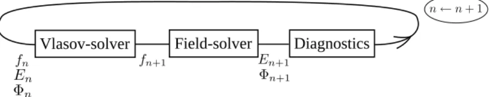
In this gyrokinetic model, the main unknown is a distribution functionf which represents the density of ions at a given phase space position. The execution of GYSELA is decomposed in an initialization phase, iterations over time, and an exit phase. Figure 1 illustrates the numerical scheme used during a time step: fn represents the distribution function, Φn the electric potential andEn
the electric field which corresponds to the derivative ofΦn. The Vlasov-solver step performs the
evolution offnover time and the Field-solver step computesEn. Periodically, GYSELAexecutes
diagnostics which export meaningful results extracted fromfn,En and saves the results in HDF5
files.
The distribution function f is a 5 dimension variable and also evolves over time. The first 3 dimensions are in space, xG= (r, θ, ϕ) with r and θ the polar coordinates in the poloidal
cross-section of the torus, while ϕ refers to the toroidal angle. The two last coordinates are in velocity space:vkthe parallel velocity along the magnetic field lines andµthe magnetic moment
(proportional tov⊥2withv⊥being the perpendicular velocity).
LetNr,Nθ,Nϕ,Nvkbe respectively the number of points in each dimensionr,θ,ϕ,vk. In the
Vlasov-solver, each value ofµis associated with a set of MPIprocesses (a MPIcommunicator).
Vlasov-solver Field-solver Diagnostics
Within each set, a 2D domain decomposition allows us to assign to each MPI process a sub-domain in (r, θ)dimensions. Thus, a MPIprocess is then responsible for the storage of the sub-domain defined by f (r = [istart, iend], θ = [jstart, jend], ϕ = ∗, vk= ∗, µ = µvalue). The parallel
decomposition is initially set up knowing local values istart, iend, jstart, jend, µvalue. These 2D
domains are derived from a classical block decomposition of the r domain intopr sub-domains
and of the θdomain intopθ sub-domains [LCGS07, LGCDP11]. The number of MPIprocesses
used during one run is equal to pr× pθ× Nµ. For some computations (diagnostics, gyroaverage
operator), we need to transpose the distribution function in order to have access to the poloidal plane (r = ∗, θ = ∗). For that purpose, we have designed a second parallel domain decomposition along vk andϕ, and also a set of routines and communication schemes to remap the distribution functionf back and forth between the two parallel domain decompositions.
The OPENMP paradigm is then used in addition to MPI(#T threads in each MPIprocess) to use fine-grained parallelism.
2.2. Analysis of memory footprint
A GYSELArun needs a large amount of memory to be executed. During a run, each MPIprocess is associated with a singleµvalue (section 2.1) and is responsible for a part of the distribution function as a 4D array and the electric field as a 3D array. The remaining of the memory consumption is mostly related to arrays used to accelerate computations, arrays that store intermediate results for diagnostics, MPIuser buffers to concatenate data for MPIsend/receive calls and OPENMP user buffers to compute temporary results. The biggest arrays are allocated during the initialization of GYSELAand are deallocated at the end of the application.
In order to better understand the memory behavior of GYSELA, we have logged each allocation
(allocate statement) by storing the array name, type and size. Using these data we have performed a strong scalingstudy presented in Table I (16threads per MPIprocess). This study consists in doing a run with a large enough mesh, in evaluating the memory consumption (for each MPIprocess) and then increasing step by step the number of MPI processes used for the simulation. Let say for a given simulation withnprocesses, we usexGiga Bytes of memory per process. In the ideal case, one can expect that the same simulation with2nprocesses would usex2 Giga Bytes of memory per process. In this case, memory scalability is considered perfect. But in practice, this is generally not the case because of memory overheads that do not scale.
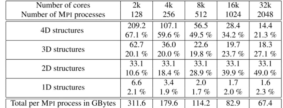
Table I. Strong scaling: allocation sizes (in GB per MPIprocess) of data allocated during initialization stage and percentage with respect to total size for each kind of data
Number of cores 2k 4k 8k 16k 32k Number of MPIprocesses 128 256 512 1024 2048 4D structures 209.2 107.1 56.5 28.4 14.4 67.1 % 59.6 % 49.5 % 34.2 % 21.3 % 3D structures 62.7 36.0 22.6 19.7 18.3 20.1 % 20.0 % 19.8 % 23.7 % 27.1 % 2D structures 33.1 33.1 33.1 33.1 33.1 10.6 % 18.4 % 28.9 % 39.9 % 49.0 % 1D structures 6.6 3.4 2.0 1.7 1.6 2.1 % 1.9 % 1.7 % 2.0 % 2.3 %
Total per MPIprocess in GBytes 311.6 179.6 114.2 82.9 67.4
Table I shows the evolution of the memory consumption along with the number of cores for a single MPIprocess. The percentage of memory consumption compared with the total memory of the process is given for each type of data structure. The dimensions of the mesh are set to
Nr= 1024, Nθ= 4096, Nϕ= 1024, Nvk= 128, Nµ= 2 . (1)
This mesh is bigger than the meshes used in production nowadays, but match further needs, especially those expected for kinetic electron physics. The last case with 2048processes requires
67.4GB of memory per MPIprocess. We usually launch a single MPI process per node, and we can notice that the memory required is largest than, for example the64GB of a Bull Helios‡ node or the16GB of an IBM Blue Gene/Q node. Table I also illustrates that 2D structures and many 1D structures do not benefit from parallelization. In fact, the memory cost of the 2D structures does not depend on the number of processes at all, but rather on the mesh size and the number of threads. On the last case with32k cores, the cost of the 2D structures is the main bottleneck, as it takes
49% of the whole memory footprint. Finally, we can point out that memory overheads observed in large simulations are due to various reasons. Additional extra memory is needed, for example, to store briefly some coefficients during an interpolation (for the Semi-Lagrangian solver of the Vlasov equation). Several MPI buffers are used whenever the application deals with the sending and the receiving of temporary data. Often, before using MPIsubroutines, a copy to reorganize and change the shape of data is required to send or receive them.
As improving the memory scalability is equivalent to decreasing the memory overheads, understand the memory consumption of GYSELAis essential. The following section gives a state of the art about profiling memory tools.
3. OVERVIEW OF THE MEMORY SCALABILITY STUDY
The study of the memory scalability for parallel applications is rather uncommon. Among the different challenges of parallel programming, the most popular one is the study of the execution time scalability; to achieve good results redarding memory scalability many analysis and a fine understanding of the data and computation flows of the application must be undertaken.
When an application scales well and can already use a large amount of cores, the study of the memory consumption can become critical. In fact, the larger the simulation, the more the cost of structures which do not scale becomes the main limiting factor to handle bigger problems.
In this section, we present the two main kinds of tools to deal with the memory scalibility issue. A description of the operating of these tools is given in the subsection 5.1.1. To deal with the memory scalability issue, two main approaches can be distinguished. On one hand a dedicated approach can be done that consists in building an integrated solution for a given application, and on the other hand the generic approach is based on the use of generic performance evaluation tools.
3.1. Different approaches to study the memory scalability
When using a dedicated solution for an application, one way to investigate the memory scalability issue is to build a reduced model of the memory consumption in function of numerical parameters of the application and of parallelization parameters of the simulation, for example the number of MPIprocesses. This approach requires deep knowledge of the application behavior. This is the main concern of paper [KPE+12] on the NESTapplication. A discussion of this approach is given below.
Another way to investigate the memory scalability issue is to instrument at the source code level. This allows us to retrieve different valuable quantities to study the scalability. For instance, in our case the memory consumption strongly depends on the parallelization parameters of the simulation. The main advantage of a dedicated solution is to perform optimizations that scale correctly, to make as few assumptions as possible to model the memory consumption, taking also into account specific issues related to the application.
Let us consider now representative generic tools like SCALASCA [GWW+10], EZTRACE
[AMGRT13], PIN [LCM+05]. These tools provide different measurements of the application, generally with small efforts from the developers (cf. subsection 5.1.1 regarding the different approaches of instrumentation), but the interpretation of these measurements are not always straightforward. Regarding the memory scalability aspect, it can be difficult to estimate how the memory consumption depends on the parallel parameters only from measurements of the total
memory consumption. Even if one knows what is the memory consumption for different parallel configurations of a simulation, using empirical extrapolation to estimate the consumption on bigger configurations is not enough accurate in many cases. The relevant information we are looking for is how the memory consumption evolves if you change a parallelization parameter, the number of MPI
processes for example. The current generic tools do not provide this kind of feature. Moreover, in the context of large parallel applications, these generic tools can be unavailable on the supercomputer used for the simulation, and even if they are available, there is no guarantee that they do not introduce a significant overhead when using a large number of processes.
In this study focusing on the memory footprint in GYSELA, we use a dedicated solution based on a source code instrumentation to investigate the memory scalability of the code. However, our final goal is to identify a generic method to build a portable and versatile tool that would be usable in other parallel applications.
3.2. Memory scalability of the massively parallel applicationNEST
In this section, we illustrate the issue brought by memory scalability with a published study on the application NEST. The application NESTsimulates the propagation of a spike in an neuronal network connected by synapses; it has been described from the memory consumption point of view in [KPE+12]. To deal with quite large networks, the memory consumption must be optimized.
To study this aspect, an expression which models the memory consumption per MPIprocess was established. The terms of this expression depend on the number of MPI processes, the number of neurons in the network and the number of incoming connexions to a neuron. Additionally, some constant parameters were introduced to quantify some untraceable memory consumptions in the implementation of NEST. Some memory allocation remained intractable in offline mode. This is the case if the size of the allocations strongly depends on the execution. In the case of NEST, some allocations are related to the path of the spike in the given neuronal network. Those allocations are modeled by constant parameters and these constants are estimated thanks to an experimental protocol. The strong point of this approach relies on the fact that with a quite small expression, one can do an accurate prediction of the memory peak of the NESTapplication over a large configuration. But this method assumes the developer has a good knowledge of the parallel application to define correctly the expression of the memory peak and it cannot be automated. So depending on the complexity of the application, this task can be difficult.
In the case of GYSELA, the memory consumption depends only on an input set of static
parameters. More details about the assumption to estimate accurately the memory consumption in offline mode are given at the end of section 4. The dedicated tools developed for GYSELA
are therefore based on an instrumentation at the source level to allow us to retrieve all necessary informations about each allocation/deallocation of the application. Compared to the work on the application NEST, our approach can be applied with a less deep knowledge of the application. Also, in our method, the prediction done by our tool reflects exactly the behavior of the application from the memory consumption point of view.
In section 4, the method used to reduce the memory consumption of GYSELA is described. Section 5 details the different features of our tools and how they contribute to study the memory consumption.
4. A METHOD TO REDUCE THE MEMORY FOOTPRINT OF GYSELA
There are at least two ways to reduce the memory footprint of a parallel application. On one hand, we can first increase the number of nodes used for the simulation, since the size of data structures which benefit from a domain decomposition will decrease along with the number of MPIprocesses. On the other hand, we can manage more finely the array allocations in order to reduce the memory costs that do not scale with the number of threads/MPI processes and to limit the impact of all allocated data at the memory peak. In fact, this approach consists of reducing the impact of memory overhead at the memory peak, and so, it improves the memory scalability of the application.
To achieve the reduction of the memory footprint and to push back the memory bottleneck, we choose to focus on the second approach. In the original version of the GYSELA code, most of the variables are allocated during the initialization phase. This procedure is rightful for structures which are for persistent variables in opposition to temporary variables that could be dynamically allocated. In this configuration, one can determine early the memory space required without actually executing a complete simulation. This allows a user to know if the case submitted can be run or not. Secondly, it avoids execution overheads due to dynamic memory management. But a disadvantage of this approach is that variables used locally in one or two subroutines consume their memory space during the whole execution of the simulation. As the memory space becomes a critical point when a large number of cores are employed, we have allocated a large subset of these variables as temporary variables with dynamic allocation. This has reduced the memory peak with a negligible impact on the execution time. However, one issue with dynamic allocations is that we lost the two main advantages of the static allocations, and particularly the ability to determine in advance the memory space required to run a simulation. Thanks to the prediction tool (section 5.3) developed for GYSELA, we recover this advantage while doing dynamic allocations.
The method we apply to reduce the memory peak of GYSELAcan be described as: Method IMPR: Incremental Memory Peak Reduction
Step 0 Choose the target configuration of the application (input parameter set), Step 1 Locate the moment of the memory peak during the execution,
Step 2 Identify the data structures allocated at the memory peak,
Step 3 Evaluate which one can be deallocated. If none of them can be simply deallocated, reconsider the algorithms used and try to improve them,
Step 4 After adding deallocations or modifying algorithms, go back to ’Step 0’.
Each step of the IMPR Method needs careful attention. Step 0 of this method has a direct impact on the other steps. From the point of view of the memory consumption in GYSELA, the crucial parameters are the size of the mesh and the number of MPIprocesses. Depending on these parameters, the memory peak settles at a specific location, this can really change the part of the code to focus on. The prediction tool (section 5.3) allows us to take the data from a run of reference and to change them offline to explore different configurations and settings easily. This feture provides the necessary information for the other steps. With this tool, we can study GYSELAin small and big configurations easily (without launching parallel jobs).
In Step 1, the location of the memory peak means to locate the lines of the source code and the call stack where the maximum memory consumption is reached. To identify the allocated data structure in Step 2, this implies to track the allocations/deallocations of all data structures used during a run. These two steps are possible thanks to our tools described in sections 5.1 and 5.2.
For Step 3, the developer has to pay attention to the data dependencies to understand which arrays can potentially be removed whenever the memory peak occurs. There are different ways to get less memory consumption. One can decide to reuse an existing temporary array, or to do more computation instead of saving a result in memory, or you can notice data duplication that can be avoided, or you can notice that some allocated buffers can be deallocated during a short time slot. If the search of these kinds of situations does not succeed, you can also conclude that the employed scheme needs too much memory and that a way of reducing the memory consumption is to change the algorithm and/or the numerical scheme. This will certainly require new developments. In the GYSELAframework, we have mainly target the data structures that penalize the application at large scale (because they do not benefit of domain decomposition). This process is illustrated in section 6. Once the source code is modified in Step 4, one can often observe a shift of the memory peak in time. So, for the next iteration of the method, we will certainly focus on another part of the application. Finally, the method loops back to the Step 0 until the memory footprint is low enough. Let us notice that in order to use the prediction tool in offline mode, a strong assumption is required: all memory allocations of the application must be independent of any variables that can vary by a non-deterministic process. In other words, given an input set of parameters, the memory behavior of the application is unique and deterministic (it does not depend on environment or intractable process). This assumption is fulfilled in the GYSELA application. If this assumption
is not available for a given application, it would require to perform the different steps of the method without the prediction tool, and then to launch as many jobs as required to generate needed trace files.
The dedicated tools developed for GYSELAallow us to investigate this IMPR Method. The next section describes more precisely these tools.
5. CUSTOMIZED MODELING AND TRACING MEMORY TOOLS
To follow up the memory consumption of GYSELA and to measure the memory footprint reduction, two different tools have been developed: a FORTRANmodule to generate a trace file of allocations/deallocations and a visualization + prediction PYTHON script which exploits the trace file. The information retrieved from the execution of GYSELAthanks to the instrumentation module is a key component of our memory analysis. The implementation of these helpful tools is detailed in following sections.
5.1. Trace File
Various data structures are used in GYSELAand in order to handle their allocations/deallocations, a dedicated FORTRANmodule was developed to log them into a file: the dynamic memory trace. As in the current implementation the MPIprocesses have almost the same dynamic memory trace, we produce a single trace file for the allocations/deallocations of MPIprocess 0.
5.1.1. Overview of generic tools. In the community of performance analysis tools dedicated to parallel applications, different approaches exist. Almost all of them rely on trace files. A trace file collects informations from the application to represent one aspect of its execution: execution time, number of MPI messages sent, idle time, memory consumption and so on. But to obtain these informations, the application has to be instrumented. The instrumentation can be made at 4 levels: in the source code, at compilation time, at linking-time or during execution (just in time).
The SCALASCA performance tool [GWW+10] is able to instrument at compilation time. This
approach has the advantage to cover all the code parts of the application and it allows the customization of the retrieved information. This systematic approach gives a full detailed trace but the main purpose of SCALASCAis to locate the bottleneck of an application, not to study the memory scalability. Also by using automatic instrumentation, it can be difficult to retrieve the expression of an allocation, like we do (cf. subsection 5.1.2).
The tool set EZTRACE [AMGRT13] offers the possibility of intercepting calls to a set of functions. This tool can quickly instrument an application thanks to a link with third-party libraries at linking-time. Unlike our approach, this one does not need an instrumentation of the code but you cannot hope to retrieve the allocation expression in this approach.
The tools PIN [LCM+05], DYNAMORIO [BGA03] or MAQAO [DBC+05] use the Just In Time (JIT) approach to instrument the application during the execution. The advantage here is the genericity of the method. Any program can be instrumented by this way, but in this approach, retrieving the expression of the size of an allocation is also an issue, as for tools based on intrumentation at linking-time.
Another software commonly used to detect memory peaks is VALGRIND [NS07]. This software uses a heavy intrusive binary instrumentation approach. This tool retrieves all the informations about the memory accesses done during the runtime of any program. Among the tools based on VALGRIND, the MASSIF tool is able to plot the memory consumption. Figure 2 of section 5.2 achieves the same goal, i.e. gives an overview of the memory consumption and locates the memory peak. Nevertheless, one drawback of the binary instrumentation is the added overheads, another one is the weak management of parallel programming issues.
The basis of a binary instrumentation is a program that has been already compiled. But, after compilation, it is difficult to find the link between the values used to size the data allocation and the variables at the source level code responsible for this allocation. This aspect is essential for
our prediction tool in order to mimic the application in offline mode. The offline prediction of the memory consumption is unavailable if one cannot bind the size of the allocated structure and the name of variables which set the dimensions of the allocations.
The tools we have developed allows us to measure the performance of GYSELA, from the memory point of view. These tools are dedicated to GYSELA and deal only with the memory scalability issue unlike the previous generic tools. The source code is instrumented thanks to a FORTRAN
module to generate a trace file at the execution. A visualization tool has been developed to deal with the provided trace file. It offers a global view of the memory consumption and an accurate view around the memory peak to help the developer to identify problems and then to reduce the memory footprint. The terminal output of the post processing script gives valuable informations about the arrays allocated when the memory peak is reached. Given a trace file, we can also extrapolate the memory consumption in function of the input parameters. This allows one to investigate the memory scalability. As far as we know, there is no equivalent tool to profile the memory behavior in the HPC community.
5.1.2. Implementation. A dedicated FORTRANinstrumentation module has been developed. This instrumentation generates a trace file. Then we perform a post-mortem analysis on it. The instrumentation module offers an interface, take and drop, which wraps the calls to allocate and deallocate. The take and drop subroutines perform the allocation and deallocation of the array handled and they log their memory action in the dynamic memory trace file.
For each allocation and deallocation, the module logs the name of the array, its type, its size and the expression of number of elements. The expression is required to make prediction. For example, the expression associated to the allocation
integer, dimension(:,:), pointer :: array
integer :: a0, a1, b0, b1
allocate(array(a0:a1, b0:b1))
is
(a1 − a0 + 1) × (b1 − b0 + 1). (2)
To be able to evaluate these allocation expressions, the variables inside them must be recorded: either the value of the variable or the arithmetical expression depending on previous recorded variables. This is done respectively by the subroutines write param and write expr. The writing of an expression saves the relationship between parameters in the trace file. This is essential for the prediction tool (section 5.3). The following code is an example for recording the parameters
a0, a1, b0, b1:
call write_param(’a0’, 1); call write_param(’a1’, 10)
call write_param(’b0’, 1); call write_expr(’b1’, ’2*(a1-a0+1)’)
To retrieve the temporal aspect of the memory allocation, the entry/exit to selected subroutines is recorded by the interface write begin sub and write end sub. This allows us to localize where the allocations/deallocations happen which is a key point for the visualization step.
5.2. Visualization tool
In order to address the memory consumption issues, we have to identify the parts of the code where the memory usage reaches its peak. The log file can be large, i.e several Mega Bytes. To manage this amount of data, a PYTHONscript was developed to visualize them. This tool helps the developer to understand the memory cost of the handled algorithms, and so gives him some hints how and where it is meaningful to decrease the memory footprint. These informations are given thanks to two kinds of plots.
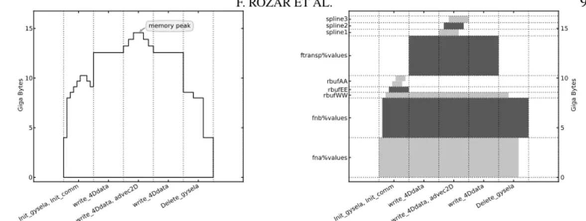
Figure 2 plots the dynamic memory consumption in GB along time for the MPI process 0. The X axis represents the chronological entry/exit of instrumented subroutines. The Y axis gives memory consumption in GB. The number of subroutines plotted on the graph has been shortened in order to improve the readability. In Figure 3, the X axis remains identical to the previous Figure, while the Y axis corresponds to the names of the array. Each array is associated with a horizontal line of the picture. The allocation of an array matches a rectangle, filled in dark or light
Figure 2. Evolution of the dynamic memory consumption during GYSELAexecution
Figure 3. Allocation and deallocation of arrays used in different GYSELAsubroutines
grey color in its corresponding line. The width of rectangles depends on the subroutines where allocation/deallocation happens.
In Figure 2 one can locate in which subroutine the memory peak is reached. In Figure 3 one can then identify the arrays that are actually allocated when the memory peak is reached. Thanks to these information, we exactly know where to modify the code in order to reduce the global memory consumption.
5.3. Prediction tool
To anticipate the memory requirements when running a given simulation, we need to predict the memory consumption with any given input parameter set. Thanks to the expressions of array size and the value or expression of numerical parameters contained in the trace file, we can model the memory behavior off-line. The idea here is to reproduce allocations from the trace file with a given input set of parameters.
Sometimes, a parameter value cannot be expressed as a one line arithmetical expression (e.g. multi criteria optimization loop to determine the value). To manage this case and in order to be faithful, the FORTRANpiece of code which returns the value is called from the PYTHONscript. This is possible thanks to a compilation of the needed FORTRANsources with f2py [Pet09].
By changing the value of input parameters, our PYTHON prediction tool offers the possibility to precisely establish the GYSELAmemory consumption for a MPIprocess on greater meshes. It also gives the possibility to calibrate the quantity of computational ressources required by a given simulation case. The prediction tool allows us to explore machine configurations which do not exist yet, such as the Exsacale ones. The results of this tool are presented in section 7.1.
6. REDUCING THE MEMORY FOOTPRINT IN GYSELA STEPWISE 6.1. Achieving memory reduction step by step
In order to reduce the memory footprint of GYSELA, we follow the IMPR Method. We are willing to cut down the memory peak at each iteration of this Method. The code changes we consider consist of moving allocations/deallocations of a set of data structures and in changing some algorithms. To track the changes concerning the location of the memory peak and the amount of memory usage after each optimization step, a reference run has been defined that uses64MPIprocesses and16
threads per process, leading to a total of1024cores. In this subsection, we will use for our analysis the maximum of memory consumption given for one MPIprocess. The mesh of the reference case is set to
Nr= 512, Nθ= 1024, Nϕ= 128, Nvk= 128, Nµ= 2 . (3)
Originally, a large fraction of the data structure allocations in GYSELAare done at application startup. These persistent data structures are allocated in the initialization step and deallocated in the exit step (as above mentioned in section 4). In this original setting, a GYSELAspecific wrapper logs
some of the allocate function calls. The name, the size and the dimensions of each allocated data structure are recorded in a trace file during the GYSELAinitialization. In this persistent allocation approach, these informations are added up to give directly the maximum of memory consumption soon after the application launch. However, this is no longer true when we insert the dynamic management of the data structure allocations. Starting with the persistent allocation trace file, we obtain Table I. It appears that 1D and 2D structures represent a large amount of the memory usage for a large run. With this original version, GYSELAexhibits a maximum memory consumption of
14.14GB. In the following, we will observe and reduce this peak memory consumption focusing on the reference case.
Let us consider a first optimization looking at data structures allocated that appear in trace files. Several 1D and 2D data structures that store intermediate computations take most of the memory space. We remove the initial allocation for these data and bring the allocation/deallocation combination closer to the usage of these data structures. The aim is to move the allocations of these data structures as close as possible to their utilization. We keep in mind that frequent calls to allocation/deallocation primitives can lead to execution time overheads. In the framework of GYSELA application, we have performed some measurements of the total execution time considering several choices for the allocation/deallocation calls; we conclude that the locations which do not introduce too much overhead are those that are just outside the OPENMP areas. This approach allows us to keep an execution time of the version with dynamic management of allocations for 1D and 2D data structures close to the static management version. As we introduce a set of arrays that are now allocated/deallocated from time to time, a memory peak appears (i.e it is a dynamic memory peak which is not known from the beginning). In this new version, the maximum memory consumption is then13.53GB.
Subsequently, we investigate a second memory optimization looking at data structures allocated at the memory peak. We notice that some 2D arrays which store the spline coefficients are allocated during the whole run while they are used only during the Vlasov solving step (the main computation kernel). In the same way than the previous optimization, we move the allocations/deallocations of the spline coefficients closer to their effective use, in order to decrease the memory peak (not located in the Vlasov solver). This modification reduces the memory peak down to11.89GB.
In the third phase of IMPR Method, we again list the data structures allocated at the memory peak. In this list, some 2D arrays store matrices that are used in the subroutines that compute the gyroaverage operator. Those matrices store precomputed values to accelerate the computation of the gyroaverage operator (precomputations are done at each GYSELAstartup). Two changes are performed: moving the allocations/deallocations of those 2D arrays near their usage and setting these arrays to their correct values just before use. Although the dynamic management of allocation and the setting of these structures introduce a small overhead in execution time, this allows us to decrease the memory peak to11.63GB.
After these successive improvements, we have reduced the memory peak by17% on the reference case. As our goal is to deal with larger meshes, we expect to provide a way to reach a better reduction. The next step described in the following subsection will highlight part of the data dependencies of GYSELA. We will identify an array that can be deallocated during a slot time to shift the memory peak location.
6.2. Further memory optimizations using data dependencies
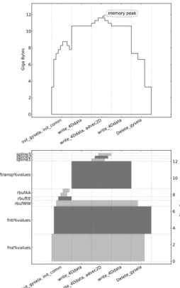
The optimizations of the previous subsection have lowered the memory consumption. We again consider the IMPR Method to investigate memory scalability. The visualization tool generates the pictures of Figure 4. These pictures are intentionally simplified to improve readability. The curves (upper part) that give memory consumption along with the time help the developer to locate the memory peak in the advec2D subroutine (a part of the Vlasov solver). In the lower part of Figure 4, the biggest allocated data structures are shown. One can wonder which of these data can be deallocated.
After an accurate analysis of the advec2D subroutine, we notice that inside the 2D advection step, a transposition of the main unknown (4D distribution function) is done to achieve the
computation of splines coefficients on the poloidal plane. By the way, we noticed that at the memory peak, the transposed data structure (named ftransp%values) and the original distribution function (named fnb%values) contain the same information stored into two different containers. Then we manage to deallocate fnb%values temporarily during the memory peak. No extra computations is required here, but the readability of the code is altered a little bit with this change. We then obtain the outputs of Figure 5. Practically, the memory peak is reduced to10.66GB. This improvement is characterized by a move of the memory peak. If one compares Figures 4 and 5, it is noticeable that the memory peak is located in a different subroutine. This detail is crucial, as it may imply to focus on another part of the code for the next iteration of the IMPR Method.
Our visualization tool gives a new point of view on the possible bottlenecks related to memory consumption. This tool helped us to iteratively reduce the memory overheads and also to improve the memory scalability.
7. RESULTS
In this section, some experimental results about the memory scalability of GYSELAare presented by a strong scaling study. In a second part, we show how the prediction tool can be used to design the configuration of a production simulation.
7.1. Memory scalability
Table II details the strong scaling test using the latest stable release-v5.0 of GYSELAthat includes the new dynamic allocation scheme and the algorithmic improvements detailed in section 6. The prediction tool allows us to reproduce the Table I on the initially targeted mesh Nr= 1024, Nθ= 4096,Nϕ= 1024,Nvk= 128,Nµ= 2.
Figure 4. Visualization of the memory trace on 1024 cores
Figure 5. After improvement, visualization of the memory trace on 1024 cores
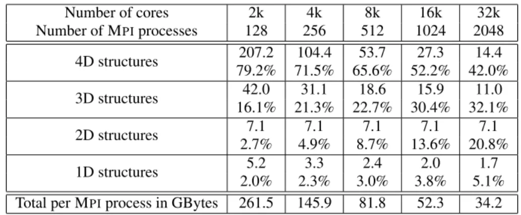
Table II. Strong scaling: memory allocation size and percentage with respect to the total for each kind of data at the memory peak
Number of cores 2k 4k 8k 16k 32k Number of MPIprocesses 128 256 512 1024 2048 4D structures 207.2 104.4 53.7 27.3 14.4 79.2% 71.5% 65.6% 52.2% 42.0% 3D structures 42.0 31.1 18.6 15.9 11.0 16.1% 21.3% 22.7% 30.4% 32.1% 2D structures 7.1 7.1 7.1 7.1 7.1 2.7% 4.9% 8.7% 13.6% 20.8% 1D structures 5.2 3.3 2.4 2.0 1.7 2.0% 2.3% 3.0% 3.8% 5.1%
Total per MPIprocess in GBytes 261.5 145.9 81.8 52.3 34.2
Table II outputs the memory consumption at the memory peak. It is obtained by keeping the mesh size constant and changing the number of MPIprocesses. For this strong scaling study in the GYSELAframework, we have to modify the domain decomposition setting in therandθdirections to increase the number of MPIprocesses. Our prediction script replays the allocations/deallocations of the trace file by recomputing the size of each array considering the new domain decomposition. The numbers given in Table II are obtained thanks to the prediction tool and moreover, they were checked with different test cases such as the bigger one that uses 32k cores.
As one can see on the biggest case (32k cores), the consumption of the 2D structures is reduced to 20.8%. Also the memory gain on this case is of 50.8% on the global consumption compared to Table I. The 4D structures contain the most relevant data used during the computation and they consume most of the memory as they should. The memory overheads have been globally reduced, this improves the memory scalability of GYSELAand allows us to run larger simulations.
Based on the feedback of different runs, the tools integrated in GYSELAand detailed in this paper
do not introduce too much execution time overheads. Nevertheless, the origin of these overheads can be identified as, firstly the cost of input/output activities on disk, and secondly the more and more frequent calls to the allocate subroutine. The second point is certainly the most important one, because to continue to decrease the memory footprint, more arrays should be allocated dynamically. The study and reduction of overheads due to dynamic allocators will be the purpose of future works. 7.2. Using prediction tool for production runs
Before launching a simulation on a supercomputer, it is helpful to know how to check the set of important parameters for a given parallel application. Indeed, the time to wait before the run can start be quite long (several days) if one asks for a lot of computing resources. Therefore, one may wonder if the application will start with well-designed parameters and if it will exceed the available memory. With the prediction tool, it is possible to evaluate for a given mesh size and an input parameter file if a GYSELAsimulation can be run (i.e fit into the available memory) or not.
To illustrate this point, we have made a larger reference run on the Juqueen§ machine and saved the associated memory trace file. The Juqueen machine is an IBM BlueGene/Q with 16 GB of memory per node. Moreover to be able to exploit most of the computational capacity of this machine, we commonly use64threads per node (16 cores).
In this large reference run, we use256MPIprocesses and64OPENMP threads (4k cores). Usually a GYSELArun is set such that a single MPIprocess is launched per node; we choose this setting
also for the other tests described in this subsection. The mesh for this run is given by
Nr= 256, Nθ= 256, Nϕ= 128, Nvk= 64, Nµ= 4 . (4)
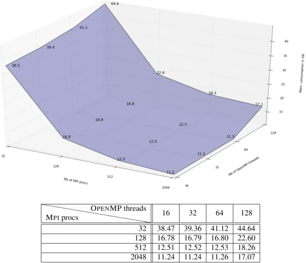
hhhhhh hhhhhh hhh MPIprocs OPENMP threads 16 32 64 128 32 38.47 39.36 41.12 44.64 128 16.78 16.79 16.80 22.60 512 12.51 12.52 12.53 18.26 2048 11.24 11.24 11.26 17.07
Figure 6. The memory peak (in GB) depending on the number of MPIprocs and of OPENMP threads
Using the trace file of this run, the behavior of the memory consumption of GYSELAcan be predicted. We would like to know a list of possible deployments that can handle the following target mesh:
Nr= 1024, Nθ= 1024, Nϕ= 128, Nvk= 64, Nµ= 4 . (5)
We change the parameters of the mesh directly in the trace file and also the number of MPI
processes and the number of OPENMP threads. Scanning a set of values, we output the memory peak per MPIprocess with the prediction tool. The obtained results are plotted on Figure 6. With the 16GB available on a Juqueen node, one can observe that from512 processes and below 64
threads, the GYSELAcode fit into the memory and can handle the targeted mesh.
Some data structure used by application for which the parallelism is induiced by the domain decomposition of the mesh can take avantage of this decomposition. This means that the cost of this kind of structure decreases as the number of process increases. On Figure 6, one can notice that the behavior of the memory consumption along the MPIprocess axis is consistent with the expected behavior. While the application uses a larger number of processes, the memory costs tend to diminish. But, a saturation effect arises between128and2048MPIprocesses. This is due to some arrays that do not scale along with the number of subdomains in(r, θ).
Along the thread axis, it is noteworthy that the number of threads has less impact on the memory peak than the number of processes. A gradual increase of the memory peak along with the number of threads is clear for32processes. Considering other numbers of processes and below64threads, the number of threads has a negligible effect on the memory peak. But we notice a sudden increase of memory consumption for all cases in between64and128threads. After an analysis of the memory
consumption along time, it appears that the memory peak is not located in the same subroutine for both cases. In the128threads setting, the memory peak depends strongly on the number of threads, whereas for64threads and below this is not the case. The move of the memory peak appears only for128threads and the prediction tool helps to detect that kind of behavior.
One of the contributions of the prediction tool that mimics accurately the real execution of the code is to quantify accurately the memory consumption and to be able to observe the move of memory peak in the offline mode. This cannot be done with an empirical model of the memory consumption as shown in the NESTapplication for example (section 3.2).
8. CONCLUSION
The work described in this paper focuses on a memory modeling and tracing module and some post processing tools which enable us to improve the memory scalability of GYSELA. With this framework, the understanding of the memory footprint behavior along time is achievable. Also, the generated trace file can be reused to extrapolate the memory consumption for different input sets of parameters in offline mode; this aspect is important both for end-users who need greater resolutions or features with greedy memory needs, and for developers to design algorithms for Exascale machine.
With these tools, a reduction of 50.8% of the memory peak has been achieved and the memory scalability of the GYSELA has been improved. Our next objective is to implement a versatile C/Fortran library. This library will provide an API to replace the standard calls to allocation/deallocation instructions in C/Fortran. It will also provide the post processing scripts to visualize the trace file and to perform predictions. As said in section 4, to use the prediction feature, the pattern of the memory footprint must depend only on an input set of parameters, not on computed values during the execution. However the visualization script does not require this assumption. An objective of the library is to prevent introducing too large execution time overhead and to be able to be used over large configurations. This next step will outsource the features we developed for tracking memory consumption in GYSELA. As our IMPR Method leads the developer to allocate his data structures dynamically, a study of the different allocators in the user space to optimize the execution time overhead should be done. Finally, the work presented in this paper is a first step towards building a general method that will help developers to improve the memory scalability of parallel applications.
REFERENCES
[ ˚ACH+13] . J. A. ˚Astr¨om, A. Carter, J. Hetherington, K. Ioakimidis, E. Lindahl, G. Mozdzynski, R. W. Nash,
P. Schlatter, A. Signell, and J. Westerholm. Preparing scientific application software for exascale computing. In Proceedings of the 11th International Conference on Applied Parallel and Scientific Computing, PARA’12, pages 27–42. Springer-Verlag, Berlin, Heidelberg, 2013.
[AMGRT13]. C. Aulagnon, D. Martin-Guillerez, F. Ru´e, and F. Trahay. Runtime function instrumentation with EZTRACE. In Euro-Par 2012: Parallel Processing Workshops, pages 395–403. Springer, 2013. [BGA03] . D. Bruening, T. Garnett, and S. Amarasinghe. An infrastructure for adaptive dynamic optimization. In
[CGO 2003], pages 265–275. IEEE, 2003.
[DBC+05] . L. Djoudi, D. Barthou, P. Carribault, C. Lemuet, J. Acquaviva, W. Jalby, et al. MAQAO: Modular
assembler quality analyzer and optimizer for itanium 2. In The 4th Workshop on EPIC architectures and compiler technology, San Jose, 2005.
[GBB+06] . V. Grandgirard, M. Brunetti, P. Bertrand, N. Besse, X. Garbet, P. Ghendrih, G. Manfredi, Y. Sarazin,
O. Sauter, E. Sonnendrucker, J. Vaclavik, and L. Villard. A drift-kinetic Semi-Lagrangian 4D code for ion turbulence simulation. Journal of Computational Physics, 217(2):395 – 423, 2006.
[GIVW10] . X. Garbet, Y. Idomura, L. Villard, and T.H. Watanabe. Gyrokinetic simulations of turbulent transport. Nuclear Fusion, 50(4):043002, 2010.
[GSG+08] . V. Grandgirard, Y. Sarazin, X. Garbet, G. Dif-Pradalier, P. Ghendrih, N. Crouseilles, G. Latu,
E. Sonnendrucker, N. Besse, and P. Bertrand. Computing ITG turbulence with a full-f semi-Lagrangian code. Communications in Nonlinear Science and Num. Sim., 13(1):81 – 87, 2008.
[GWW+10]. M. Geimer, F. Wolf, B. JN Wylie, E. ´Abrah´am, D. Becker, and B. Mohr. The SCALASCA performance
toolset architecture. CCPE, 22(6):702–719, 2010.
[Hah88] . T. S. Hahm. Nonlinear gyrokinetic equations for tokamak microturbulence. Physics of Fluids, 31(9):2670–2673, 1988.
[KPE+12] . S. Kunkel, T. C Potjans, J. M. Eppler, H. E. Plesser, A. Morrison, and M. Diesmann. Meeting the memory
challenges of brain-scale network simulation. Frontiers in neuroinformatics, 5:35, 2012.
[LCGS07] . G. Latu, N. Crouseilles, V. Grandgirard, and E. Sonnendrucker. Gyrokinetic semi-Lagrangian parallel simulation using a hybrid OpenMP/MPI programming. In Recent Advances in PVM and MPI, volume 4757 of Lecture Notes in Computer Science, pages 356–364. Springer, 2007.
[LCM+05] . C. Luk, R. Cohn, R. Muth, H. Patil, A. Klauser, G. Lowney, S. Wallace, V. J. Reddi, and K. Hazelwood.
PIN: building customized program analysis tools with dynamic instrumentation. In ACM SIGPLAN Notices, volume 40, pages 190–200. ACM, 2005.
[LGCDP11]. G. Latu, V. Grandgirard, N. Crouseilles, and G. Dif-Pradalier. Scalable quasineutral solver for gyrokinetic simulation. In PPAM (2), LNCS 7204, pages 221–231. Springer, 2011.
[NS07] . N. Nethercote and J. Seward. VALGRIND: a framework for heavyweight dynamic binary instrumentation. In ACM Sigplan Notices, volume 42, pages 89–100. ACM, 2007.
[Pet09] . P. Peterson. F2PY: a tool for connecting FORTRAN and PYTHON programs. International Journal of Computational Science and Engineering, 4(4):296–305, 2009.
[RLR14] . F. Rozar, G. Latu, and J. Roman. Achieving memory scalability in the gysela code to fit exascale constraints. In Roman Wyrzykowski, Jack Dongarra, Konrad Karczewski, and Jerzy Waniewski, editors, Parallel Processing and Applied Mathematics, Lecture Notes in Computer Science, pages 185–195. Springer Berlin Heidelberg, 2014.
[SDM11] . J. Shalf, S. Dosanjh, and J. Morrison. Exascale computing technology challenges. In High Performance Computing for Computational Science – VECPAR 2010, LNCS 6449, pages 1–25. Springer, 2011.