HAL Id: halshs-03040260
https://halshs.archives-ouvertes.fr/halshs-03040260
Preprint submitted on 4 Dec 2020
HAL is a multi-disciplinary open access archive for the deposit and dissemination of sci-entific research documents, whether they are pub-lished or not. The documents may come from teaching and research institutions in France or abroad, or from public or private research centers.
L’archive ouverte pluridisciplinaire HAL, est destinée au dépôt et à la diffusion de documents scientifiques de niveau recherche, publiés ou non, émanant des établissements d’enseignement et de recherche français ou étrangers, des laboratoires publics ou privés.
Estimation of threshold distributions for market
participation
Mattia Guerini, Patrick Musso, Lionel Nesta
To cite this version:
Mattia Guerini, Patrick Musso, Lionel Nesta. Estimation of threshold distributions for market par-ticipation. 2020. �halshs-03040260�
ESTIMATION OF THRESHOLD
DISTRIBUTIONS FOR MARKET
PARTICIPATION
Documents de travail GREDEG
GREDEG Working Papers Series
Mattia Guerini
Patrick Musso
Lionel Nesta
GREDEG WP No. 2020-21
https://ideas.repec.org/s/gre/wpaper.htmlLes opinions exprimées dans la série des Documents de travail GREDEG sont celles des auteurs et ne reflèlent pas nécessairement celles de l’institution. Les documents n’ont pas été soumis à un rapport formel et sont donc inclus dans cette série pour obtenir des commentaires et encourager la discussion. Les droits sur les documents appartiennent aux auteurs.
Estimation of Threshold Distributions for Market
Participation
Mattia Guerinia,b,c Patrick Mussoa Lionel Nestaa,b,d
aUniversité Côte dAzur, CNRS, GREDEG bOFCE, SciencesPo
cSant’Anna School of Advanced Studies dSKEMA Business School
GREDEG Working Paper No. 2020–21
Abstract
We develop a new method to estimate the parameters of threshold distributions for market participation based upon an agent-specific attribute and its decision outcome. This method requires few behavioral assumptions, is not data demanding, and can adapt to vari-ous parametric distributions. Monte Carlo simulations show that the algorithm successfully recovers three different parametric distributions and is resilient to assumption violations. An application to export decisions by French firms shows that threshold distributions are generally right-skewed. We then reveal the asymmetric effects of past policies over different quantiles of the threshold distributions.
Keywords:Parametric Distributions of Thresholds, Maximum Likelihood Estimation, Fixed Costs, Export Decision.
JEL Codes:C40, D01, F14.
B Mattia Guerini –mattia.guerini@univ-cotedazur.fr. B Patrick Musso –patrick.musso@univ-cotedazur.fr. B Lionel Nesta –lionel.nesta@univ-cotedazur.fr.
Mattia Guerini has received funding from the European Union’s Horizon 2020 research and innovation programme under the Marie Sklodowska-Curie grant agreement No 799412 (ACEPOL). This work is supported by a public grant overseen by the French National Research Agency (ANR) as part of the “Investissements davenir ” program (reference : ANR-10-EQPX-17 Centre daccès sécurisé aux données CASD). The usual disclaimers apply.
1
Introduction
Most economic activities entail sunk and fixed costs stemming from the existence of technical, regulatory and information barriers. Such barriers hinder the participation of agents in market activities and bear serious welfare implications. From a static viewpoint, these may artificially protect incumbents over potential entrants, thereby augmenting firm market power, increasing prices and/or lowering quantities. From a dynamic viewpoint, participation costs may allow incumbents to embark on uncertain and risky investments with potentially substantial sunk costs, such as research and development activities. In all circumstances, knowledge of the costs associated with market participation has immediate policy implications.
Whether agents decide to participate in a specific market – be it the product, labor, technol-ogy or financial market – depends on their ability to cover such costs. Past contributions have attempted to estimate the costs of market participation. Das et al.(2007) develop a structural model that allows the empirical estimations of sunk and fixed costs of exporting for Colombian manufacturing firms. They find that sunk entry costs into export markets amount to, on aver-age, $400 thousand, while the fixed costs appear to be negligible. Using a dynamic model of optimal stock market participation,Khorunzhina(2013) estimates that stock market participa-tion costs for consumers amount to 4-6% of labor income. More recently, Fan and Xiao(2015) estimate that entry costs in the US local telephone industry reach $6.5 million.
In this paper, we focus on market participation thresholds, not on participation costs. Thresh-olds can be defined as unobservable barriers that condition the market participation of an eco-nomic actor. An agent will participate in the market only if some of her attribute – say produc-tivity – exceeds the required threshold value of producproduc-tivity. Conversely if an agent’s attribute falls short of the threshold, she will choose not to participate in the market – or to exit it. Hence, it is the gap between the agent-specific attribute and the threshold value that ultimately dictates the decision.
Thresholds are thus well suited to represent, in a concise fashion, the arbitrage underlying market participation for one chief reason. Because they are different from costs, thresholds can be expressed in various dimensions and can be easily adapted to different settings.1 Possible examples include, inter alia, the presence of a minimum efficiency for a firm to participate in foreign markets (Eaton et al.,2011); the existence of a minimum efficient plant size to enter an
1The difference between thresholds and costs is that the former are measured over a conditioning attribute
industry (Lyons,1980); a required level of absorptive capacity for a firm to efficiently assimi-late new technologies (Cohen and Levinthal,1989); the availability of sufficient collateral for a bank to grant a loan (Jiménez et al.,2006); and the presence of a wage offer above the reserva-tion wage for a worker to accept it (DellaVigna et al.,2017). In all these instances, thresholds represent a minimum value above (below) which an economic agent decides (not) to partici-pate in a given market.
The major problem is that thresholds are empirically unobservable to social scientists or policy makers. When an economic agent truly makes her participation decisions according to a threshold problem, the external observer can only witness the decision outcome itself, and certainly not the threshold per se. Most often, thresholds appear as a theoretical parameter that firms must overcome to participate in market activities (e.g.,Melitz and Ottaviano,2008, for ex-port markets). In some instances, specific surveys may explicitly focus on particular thresholds. In their analysis of wage formation and unemployment, Brown and Taylor(2013) exploit in-formation on individual-specific reservation wages obtained from the British Household Panel Survey (BHPS), a nationally representative random sample survey of more than 5000 private households to elicit participation thresholds. However because of the setup costs for data gen-eration, existence of such information remains necessarily limited in size and scope.
This paper presents a new method to estimate the parameters of an underlying distribution of thresholds that hinder market participation. Key to our approach is the intuition that such thresholds are agent-specific rather than common to all or a group of agents. The immedi-ate consequence is that rather than estimating one threshold only, we estimimmedi-ate the parameters underlying threshold distributions. Specifically, we develop a parametric method where the observation of (i) the agents’ decision outcomes and (ii) some individual characteristics of the decision makers fostering market participation are sufficient information for recovering the statistical properties of the underlying threshold distribution. The distinctive feature of our method lies in the absence of strong requirements: it needs few behavioral assumptions, it is not data demanding, and it can adapt to various parametric distributions, institutional contexts and, more important, markets.
Knowledge of threshold distributions is important for policy makers. Imagine two dis-tributions with similar average values; however, one is symmetric, while the other exhibits right skewness. In the symmetric distribution, all agents cluster around the mean with a given standard deviation. In the asymmetric distribution, most agents cluster around the mode, but
some agents face particularly high thresholds inhibiting market participation. The policy re-sponses to these two distributions may vary substantially. In the former case, nondiscrimina-tory/general policies designed to affect the common factors of all individual thresholds should presumably be favored. In the latter case, discriminatory/targeted policies focusing on specific agents might instead be privileged. Therefore, decisions on whether to implement discrimina-tory or nondiscriminadiscrimina-tory policies should be grounded on a knowledge of the entire shape of the threshold distribution that goes beyond the first two moments.
Our contribution is fourfold. First, we develop a parametric maximum likelihood esti-mation (MLE) method to reveal the underlying parameters characterizing threshold distribu-tions. Conditional on the agent’s decision outcome and a critical variable called the θ-attribute, we derive a likelihood function that allows the recovery of the concealed threshold distribu-tion. Importantly, we make use ofVuong(1989) procedure to select the most qualified density among the various candidate distribution laws. Second, we use stochastic Monte Carlo simu-lations to study the reliability of our approach when two important underlying assumptions – one distributional and one behavioral – are violated, and we broadly define the boundaries of its application. Third, we provide a primer empirical application to the problem of export thresholds. The existing literature on international trade generally assumes the existence of fixed/sunk costs associated with export activities. We detect and estimate threshold distri-butions at the sectoral level documenting significant right-skewness and leptokurtosis within most industries. Fourth, we employ year by year estimates to investigate the possible effects of policy shocks on different quantiles of threshold distributions. Overall, our results indicate that accounting for agents’ heterogeneity and for higher order moments allows one to gain valuable information regarding the discriminatory aspect of policies.
This paper is structured as follows. Section2 formally describes the economic problem under consideration and the tool employed to solve it. Section 3 presents the rationale for Monte Carlo exercises and their results. An empirical application of our strategy to the export decision problem of French firms is presented in Section4, together with an exercise designed to explain participation rates through the moments of the threshold distributions. Section 5
2
Econometric Strategy
2.1 The intuition
We consider a series of agents i = 1, . . . , N making an economic decision, the outcome of which can be encoded as a binary variable χi ∈ {0, 1} representing their market participation.
Each agent is characterized by a specific attribute θithat affects the decision outcome. This
θ-attribute can be considered a single characteristic or a combination of several distinct features that ease or hinder the realization of a positive outcome χi = 1. We assume that an agent
decides to participate only when the θ-attribute is sufficiently large that it exceeds threshold
ci. Conversely, if an agent’s attribute falls short of the threshold, the agent will choose not to
participate in the market. Thresholds can thus be defined as unobservable barriers that dictate the market participation of an economic agent. What we call the perfect sorting hypothesis can be formalized as follows: χi= 1 if θi≥ ci χi= 0 if θi< ci (1)
The theoretical economic literature typically assumes homogeneous thresholds across agents – i.e., ci ∼ δ, with δ representing the Dirac delta distribution (seePissarides,1974;McDonald
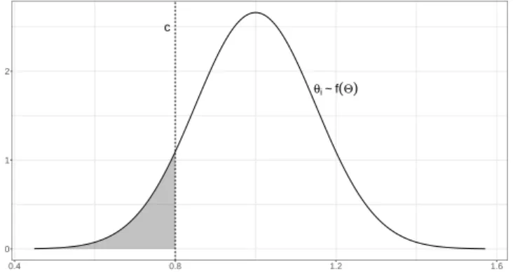
and Siegel,1986;Dixit,1989, as early developers of such an approach).2 Figure1describes this particular case by assuming an agent-specific, normally distributed θi and a unique threshold
c. The shaded area highlights the part of the distribution where all the agents withdraw from the market (χi = 0) over the θ-attribute domain (θi < c). This representation implies a
com-plete separation of agents, where only those whose θi values exceed threshold c participate in
the market.
[Figure 1 about here.]
From an empirical perspective, the issue is that the social scientist observes the decision outcome χiand the agent’s θ-attribute. However, in most situations, the threshold variable ciis
the private information of the decision maker and is thus unobservable to the external observer. This is why the empirical literature has instead focused on the probability of an agent’s market
2To the best of our knowledge,Cogan(1981) is the sole work to have estimated heterogeneous thresholds in the
participation, conditional on her θ-attribute (e.g., Kau and Hill, 1972;Wei and Timmermans,
2008, among a large series of papers). This type of exercise is technically straightforward using, for example, a simple probit model. This approach matches the fraction of actors with a positive (negative) decision outcome with the θ-attribute and produces the probability of participation conditional on the θ-attribute: P (χ = 1|θi). The caveat is that such a modeling approach cannot
reveal the threshold distribution per se.
Furthermore, evidence in several empirical fields – in particular those on the efficiency of exporters (Bernard and Jensen, 2004) and the efficiency of labor market bargaining processes (Alogoskoufis and Manning,1991) – generally contradicts the simple implication that nonpar-ticipating agents locate in the left tail of the θ distribution, whereas parnonpar-ticipating agents locate in the right tail. The rule appears to be that some agents well-endowed in their θ-attribute do not participate in a given market, and conversely, some poorly endowed agents nevertheless choose to participate. In other words, the supports of the two populations significantly overlap. To account for this persistent overlap, one must relax the assumption of a unique threshold and favor the converse assumption that thresholds are, instead, agent-specific, as is done, for ex-ample, in the theoretical work ofMayer et al.(2014). This makes it possible that well-endowed agents choose to withdraw from a market, given that their specific threshold ci exceeds their
own θ-attribute or, conversely, that poorly endowed agents choose to participate.
Assuming away the homogeneity of thresholds represents an opportunity to shift the tradi-tional perspective of Figure1. Our perspective inverts the representation proposed by Figure1
of the θ distribution and a unique threshold c. Figure2now takes the observed, agent-specific
θ-attribute as given and locates it in an unknown distribution of agent-specific thresholds ci.3
The left panel represents the case where an agent participates in a given market. Given θi,
ob-serving a positive decision outcome χi = 1implies that agent-specific threshold ci is located
somewhere to the left of θi, as indicated by the shaded area. The right panel represents the
converse: given the attribute θi, observing a negative decision outcome χi = 0implies that
agent-specific threshold ciis located to the right of θi, as indicated by the shaded area.
[Figure 2 about here.]
Our framework does not change the fundamental mechanism at work, since Equation1
holds. However, it allows the implementation of a new strategy that can estimate threshold
3
distributions by means of maximum likelihood estimation, where the parameters of interest are those that define the whole threshold distribution.
2.2 The formal model
We define the probability of an agent participating in the market as the probability that the unobserved, agent-specific threshold ciis lower than the agent-specific attribute θi:
p(χ = 1|θi) = F (θi; Ω), (2)
where F represents the cumulative density function of the probability distribution f and Ω is the vector of distribution-specific parameters to be estimated. In turn, the probability that the unobserved, agent-specific threshold ciis higher than the agent-specific attribute θiis:
p(χ = 0|θi) = 1− F (θi; Ω). (3)
The likelihood function L(Ω) then takes the generic form:
L(Ω; θi, χi) = N
∏
i=1
[F (θi; Ω)]χi× [1 − F (θi; Ω)]1−χi (4)
The log-likelihood ℓ function reads:
ℓ(Ω; θi, χi) = N
∑
i=1
χilog [F (θi; Ω)] + (1− χi) log [1− F (θi; Ω)] (5)
The decision for the social scientist is to choose a given parametric density function f (Ω), where Ω is the vector of parameters characterizing the distribution f . Given f , the objective function is that of estimating Ω such that ˆΩ = arg max
Ω ˆ
L(Ω; χi, θi).
We have two remarks. First, an important ingredient of our framework is the monotonic-ity of the relationship between the probabilmonotonic-ity of participating in a given market and the θ-attribute. If monotonicity is not empirically verified, then our behavioral assumption formal-ized in Equation1does not hold, and the corresponding likelihood function L(Ω) will prove difficult to converge. Besides, the case in which the θ-attribute is a limiting rather than an en-hancing factor can easily be envisaged. The formal model simply becomes the complement of Equation1.4
4
Second, in the case in which the cumulative distribution function is Gaussian, Equation4
resembles a traditional probit model. However, it differs from it in two important aspects. On the one hand, in a probit model, one assumes specific values for Ω by setting µ = 0 and σ = 1, whereas in our case, our aim is to estimate Ω. On the other hand, while in our framework, the domain of the support is fully observed with the vector of agent-specific attribute θi, in
a probit model, the support of the distribution is an unobserved domain. Given a vector of explanatory variables Z and a decision variable yi, the objective function of the probit model is
then to choose a vector β such that ˆβ = arg max
β
ˆ
L(β; Z, yi|µ = 0, σ = 1).5
Taking stock of the above, our framework relies on the following core assumptions:
• Assumption A1. Agents are heterogeneous in their θ-attribute θi.
• Assumption A2. Thresholds are agent-specific (ci) and follow a density distribution f
with unknown vector of parameters Ω: C ∼ F (Ω).
• Assumption A3. The relationship between the probability of participating in a market
and the θ-attribute is either monotonically increasing p(χ = 1|θi) > p(χ = 1|θj),∀θi > θj,
as in the case of an enhancing θ-attribute, or monotonically decreasing p(χ = 1|θi) <
p(χ = 1|θj),∀θi > θj, as in the case of a limiting θ-attribute.
• Assumption A4. Agents decide to participate if and only if their specific attribute θi
exceeds (is below) threshold ci(perfect sorting hypothesis).
Provided that Assumptions A1-A4 hold, the observation of vector χ = (χ1, . . . , χi, . . . , χN)
stacking all decision outcomes χiand vector θ = (θ1, . . . , θi, . . . , θN)of agent-specific attributes
θi is sufficient information to estimate the vector of parameters Ω defining the underlying
threshold distribution F . Hence the distinctive feature of our method resides in the absence
ℓ(Ω) = N ∑ i=1 (1− χi) log [F (θi; Ω)] + χilog [1− F (θi; Ω)] 5
In fact, the probit model is often presented as being derived from an underlying latent variable model similar to Equation1. Using our notation and modelling strategy in the context of a latent variable, the decision outcome χi
is set to unity if threshold c∗i < 0, and to zero otherwise. This implies that agent i participates only if the threshold
is negative. Variable c∗i is unobserved but defined as a linear function of – in our case – the θ-attribute such that
c∗i = β0+ β1θi+ zi. If ziis modelled as a standard normal, then the model reads: p(χ = 1|θi) = p(c∗i < 0|θ) =
p(zi < −(β0+ β1θi)). If z ∼ N (0, 1), then p(zi < −(β0+ β1θi)) = Fz(−(β0+ β1θi)), where Fz is the standard
normal cumulative function, and p(χ = 1|θi) = F (θi|µ = 0, σ = 1). The corresponding likelihood function is
equivalent to our Equation4, the only difference being in the parameter vector Ω. The direct implication of this is that our framework, when using the normal distribution function as our prior density, and the probit model yield exactly the same log-likelihood value. This is not surprising given that we exploit the same information in the data.
of strong requirements: it needs few behavioral assumptions, it is not data demanding, and it can adapt to various parametric distributions.
2.3 Model selection
The critical choice concerns the distribution of thresholds, as the scientist may choose among a large series of data generating processes. In the absence of prior information about the true distribution of thresholds, we rely on Vuong’s test (Vuong,1989) for the selection of non-nested models. The attractive features of Vuong’s test in our framework is twofold: (i) it does not require preexisting knowledge of the true density; (ii) it is directional, allowing one to arbitrate between any pair of assumed density functions.
The starting point is to select, among two candidate densities fp and fq, the model that is
closest to the true, unknown, density f0. The statistic tests the null hypothesis H
0that the two
models (fpand fq) are equally close to the true data generating process, against the alternative
that one model is closer. We write:
H0 :E0 [ logfp(χi|θi, Ω ∗ fp) fq(χi|θi, Ω∗fq) ] = 0, (6)
whereE0 is the expectation indicator, and Ω∗
f is the candidate, pseudo-value of the true vector
Ω. Interestingly, Equation 6 does not necessitate knowledge of the true the true density f0,
but it provides information about the best model between the alternatives fp and fq. Under
the null hypothesis, the distributions Fp and Fqare equivalent (Fp ∼ Fq). The two directional
hypotheses read: HFp :E 0 [ logfp(χi|θi, Ω ∗ fp) fq(χi|θi, Ω∗fq) ] > 0, (7)
meaning that Fpis a better fit than Fq(F1 ≻ Fq), and:
HFq :E 0 [ logfp(χi|θi, Ω ∗ fp) fq(χi|θi, Ω∗fq) ] < 0, (8)
meaning that Fqis a better fit than Fp(Fp ≺ Fq).Vuong(1989) shows that the indicatorE0 can
log LR( ˆΩfp, ˆΩfq) = ℓp( ˆΩfp)− ℓq( ˆΩfq) = N ∑ i=1 ( ℓp,i(χi|θi, ˆΩfp)− ℓq,i(χi|θi, ˆΩfq) ) = N ∑ i=1 dℓi, (9)
where ℓp,i(χi|θi, ˆΩfp)(resp. ℓq,i(χi|θi, ˆΩfq)) is observation i’s contribution to the log likelihood
ℓp (resp. lq) using density fp (resp. fq). The ratio dℓi simply represents the difference in the
log-contributions of the ith observation. In addition, Vuong (1989) suggests to account for
differences in the number of parameters in the two models as the in the Akaike Information Criterion such that:
log ˜LR( ˆΩfp, ˆΩfq) = log LR( ˆΩfp, ˆΩfq)− (kp− kq)
log N
2 (10)
where kpand kqrepresent the number of parameters in density functions fpand fq, respectively.
Given the above setting, Vuong’s z statistic reads:
Vuong’s z = (σdl
√
N )−1log ˜LR( ˆΩfp, ˆΩfq) (11)
where σdl is the standard deviation of dl. Vuong test statistic is asymptotically normally
dis-tributed by the central limit theorem. In other words, cumulative function Fp is preferred over
cumulative density function Fqif Vuong’s z exceed the (1− α)thpercentile of the standard
nor-mal distribution. Setting a 5% significance level, the corresponding z statistic in a bilateral test is|z| >= 1.96.
A last attractive feature of Vuong’s test for the selection of non-nested models is that the ranking between any pair of models is transitive. This implies that if Fp is preferred over Fq,
and Fqis preferred over Fr, then Fpis preferred over Fr.6 This is relevant in that our method can
envisage a large number of density functions and then recover a complete rank order between the competing models. If Nf densities are being tested, Nf× (Nf− 1)/2 pairwise comparisons
will allow one to recover a complete rank order of preferences across the competing density functions.
6
This is true for what concerns the comparisons of l scores. In few cases, the transitivity may be affected by the denominator of Vuong’s z, that is, the standard deviation of individual log difference σdl.
3
Monte Carlo Simulations
3.1 Monte Carlo settings
The first choice concerns the candidate parametric densities to fit to the data. The number of candidate distribution being virtually infinite, we arbitrarily choose parametric densities with two parameters only. Remember, however, that our framework can easily adapt to parametric density functions which include a higher number of parameters.
We simulate the heterogeneous threshold distribution F as extracted from three distribu-tion densities: the normal distribudistribu-tionN , the gamma distribution Γ, and the beta distribution
B: F ∈ {N ; Γ; B}. The choice of the normal, gamma and beta distributions for thresholds is
motivated by the fact that they allow us to compare a symmetric distribution in the case of the normal and asymmetric distributions of thresholds in the case of the gamma and the beta. In addition, the gamma, being very flexible, envisages various distributional shapes that may prove empirically relevant in the presence of right-skewness. The choice of the gamma also implies that we constrain the support of θ-attributes to be strictly positive: θ ∈ R+. The beta distribution is by far the most flexible, as it encapsulates all sorts of distribution shapes, ranging from left-skewed, symmetric or right-skewed distribution. The inclusion of the beta distribu-tion implies that the support lies over the 0-1 segment: θ ∈ (0, 1). This is extremely binding, because it implies that the cumulative distribution function be unity when θ exceeds one.
Following the description in Appendix A, we fix the number of agents to N = 50, 000, the number of Monte Carlo simulations to M = 1, 000, and impose a normally distributed θ-attribute θ ∼ N (.5, .15).7 In our simulation, threshold C is random variable drawn from: (i) a normal distribution with µ = .7 and σ = .2, i.e. C ∼ N (.7, .2); (ii) a right-skewed gamma distribution with shape and scale parameters αΓ = .1.5and βΓ = .5, i.e. C ∼ Γ(1.5, .5); (iii) a
left-skewed beta distribution with shape-one and shape-two parameters αB = 5and βB = 2, i.e.
C ∼ B(5, 2). For all three threshold distributions, given the vector of θ-attribute, we computed
the vector of decision outcomes χ according to Equation1.8
In what follows, we conduct several Monte Carlo simulation exercises to investigate whether the estimation of Equation5holds when Assumptions A1-A4 hold. We then explore the
robust-7We verified that our results are qualitatively robust to alternative distributions of θ
i. We tested Θ ∼
U(min, max), Θ ∼ B(α, β), and Θ ∼ P(min, α) where U, B, P represent the uniform, beta and Pareto type-II
distributions, respectively. The results are available from the authors upon request.
ness of the estimator under violations of certain assumptions.
3.2 Baseline results
We begin with a perfect scenario, where all Assumptions A1-A4 hold. Using only limited information θ and χ, we then apply our MLE algorithm to estimate the vector of parameters Ω = {µ, σ} for the Gaussian case, Ω = {αΓ, βΓ} for the gamma case and Ω = {αB, βB} for
the beta case.9 The distributions of the estimated parameters across M = 1000 Monte Carlo simulations are displayed in the different panels of Figures 3for the normal, the gamma and the beta scenarios, respectively.
[Figure 3 about here.]
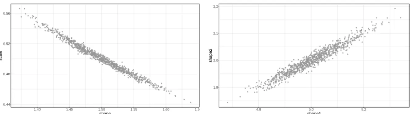
Figure3shows that, on average, our estimation strategy accurately estimates the true pa-rameters. In fact, a simple t-test never rejects the null hypothesis of equality of the estimated parameters with the target, true, parameter. However, the MLE approach provides evidence that our framework can sometimes be off target, i.e., it over- or underestimates the true pa-rameters in a magnitude reaching approximately 10% of the true parameter, especially for the gamma and beta cases. A closer inspection of the results suggests that this is due to a strong – respectively negative and positive for the gamma and the beta distributions – correlation be-tween the parameters α and β. As shown in Figure 4, there is a tight negative relationship linking the estimates of the two parameters in the gamma case (left panel) and for the beta case (right panel). Thus in the gamma case, when one of the two parameters is underestimated with respect to the true value, the other compensates and becomes overestimated. In the beta case the compensation effect goes instead in the same direction.
[Figure 4 about here.]
This compensation mechanism is a positive feature of the two asymmetric distributions. The depicted correlation between α and β simply signifies that there are several parameter combinations that allow us to unravel the density function f sufficiently close to the true one.
In Section3.3we move towards imperfect scenarios, testing the robustness of the estimation when at least one of the assumptions fails. We focus on Assumptions A2 and A4, which may prove hard to meet.
9Note that estimations of α and β for the gamma and the beta distributions allow one to analytically retrieve the
3.3 Violations of assumptions
3.3.1 Violation of A2
Assumption A2 concerns the functional form f of the threshold distribution. Since thresholds are unobservable, we need a prior concerning the density function. A specification error occurs when a functional form f assumed by the scientist is different from the true one. Without a strong prior, any probability distribution is eligible. Given this uncertainty, understanding the consequences of a violated Assumption A2 is of crucial importance. Our intuition is that the probability density function f must be sufficiently flexible to encompass a variety of shapes, so that it can adapt from case to case.
We set N = 50, 000 agents and run M = 1, 000 Monte Carlo simulations, comparing three alternatives for the likelihood function where the cumulative distribution function F may be either a normal, a gamma or a beta distribution F = {N (µ, σ), Γ(αΓ, βΓ),B(αB, βB)}. This
represents our prior about the threshold distribution. In turn, the true distribution of thresholds
C may alternatively follow a normal, a gamma or a beta distribution. For the gamma case, we consider a parametric configuration giving rise to a right-skewness with a fat right tail. For the beta distribution instead, we choose a left-skewed distribution. We set the θ-attribute such that it follows a normal distribution: θ ∼ N (.5, .0225). The set of parameters for threshold distributions is the following: (i) C ∼ N (.7, .04); (ii) C ∼ Γ(1.5, .5); and (iii) C ∼ B(5, 2).10 Combining all the possible choices for the prior F and the true distribution of C, we obtain nine different cases. In three of them, Assumption A2 is satisfied and give rise to the situations observed in the previous section. In six of them, Assumption A2 is violated.
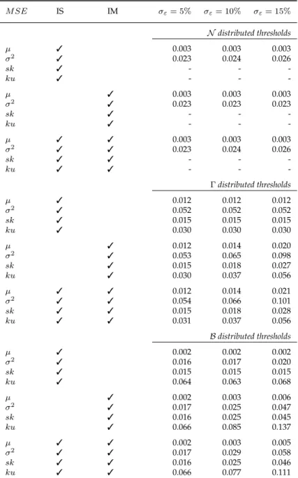
To evaluate the performance of our framework under a violation of Assumption A2, we are restricted to compare the moments estimated by our densities, since one cannot estimate the parameters of the normal distribution (µ and σ) using a gamma or an beta prior. Instead, we compute the root mean squared errors (RMSEs) of the estimated first four moments (the mean
µ; the variance σ2; the skewness sk; and the excess kurtosis k) and compare the estimated
val-ues with their true counterparts. We do this for all the scenarios combining our prior, assumed, density for the MLE exercise and the true densities. The results displayed in Table1thoroughly corroborate the results of the previous section. Absent a misspecification, the true moments are
10The guidelines for the algorithm followed for this Monte Carlo exercise are presented in the AppendixA.
Values for the variance σ2
in the normal distribution stem from setting σ to .15 for θ and .2 for the threshold normal distributions.
consistently recovered. However, when the false prior is used, a significant error is always present.
The first three rows of the bottom panel display the performance of the three priors (F =
{N (µ, σ), Γ(αΓ, βΓ),B(αB, βB)}) when the normal density is true. Consistently with Section3.2,
it shows that the normal prior performs well at recovering the first two moments of the true normal, with errors amounting to only .3% and 2.3% of the true mean and variance, respec-tively. Under violation of Assumption A2, the beta prior (with 2% and 24% errors for mean and variance, respectively) outperforms the gamma prior (with errors amounting to 5% and 53%, respectively). Our interpretation is that the beta prior outperforms the gamma one due to the impossibility of the latter to recover symmetric distributions.
We then investigate the case where thresholds are gamma distributed. Not surprisingly, the gamma prior properly recovers the first four moments. The largest RMSE concerns the second moment and reaches 5.2% of the true variance. Instead, both the normal and beta priors deteriorate when applied to a gamma distribution. This observation spans over all investigated moments: errors amounting to 20% and 23% of the true mean, and errors for all higher order moments exceed 100% of the true moments. This is due to two conditions. First, it is impossible for the normal prior to recover asymmetric and fat tailed distributions. Second, it is impossible for a beta prior to recover distribution outside the 0-1 support. The final three rows presents the results under a true beta distribution of thresholds. Our previous observation also prevail in this case. The beta prior under a true beta distribution performs well, whereas the normal and gamma priors fail in accurately estimating the first four moments of the distribution.
[Table 1 about here.]
The conclusion of the simulation exercise is clear: without proper knowledge about the true threshold distribution, misspecification can generate off-target predictions, leading to a wrong inference about participation threshold distributions. In this context,Vuong(1989) likelihood ratio test for model selection is fully advocated in order to recover a complete ranking of the candidate densities.
Table2presents the relative frequencies of each ranking of distributions, according to the
Vuong(1989) test using the simulations used above. Similarly to the sensitivity (detecting true positives) and specificity (detecting true negatives) of a test, this exercise investigates whether Vuong’s procedure correctly discriminates between the three alternative densities. Table2
re-ports the results. We observe that the test is successful at pointing to the correct true density, with the exception of only two cases in the 3, 000 simulation runs. Besides, the ranking of the two remaining alternatives are, in the vast majority of cases, consistent with the percentage errors reported in Table 1. When the true distribution of thresholds is normal, the order of preference isN ≻ B ≻ Γ in the majority of cases; when the thresholds are gamma distributed, then Γ ≻ N ≻ B is the typical ranking; and when the true density of thresholds is the beta distribution, then B ≻ N ≻ Γ is the emerging ranking. In all instances, the sensitivity and specificity of Vuong’s test hold under violations of Assumption A2.
[Table 2 about here.]
Confident that: (i) in the absence of a specification error, one can use the MLE to consistently recover the true parameters, and (ii) Vuong’s test for model selection successfully discriminates between competing prior densities, our procedure allows one to estimate participation thresh-olds in various empirical setups.
3.3.2 Violation of A4
Assumption A4 concerns the decision process of economic agents and relates to the information set available either to the entrepreneur or to the external investigator. We examine two potential sources that may affect the robustness of the estimation framework.
The first source of imperfect sorting arises when economic agents have limited information about either their own threshold ci or their own θ-attribute.11 The immediate consequence is
that agents base their decision on an erroneous inference, violating the perfect sorting hypoth-esis. We define a sorting error as a situation in which agent i, characterized by θi > ci (resp.
θi < ci), selects the negative (resp. positive) outcome χi due to agent i having an imperfect
evaluation of her threshold ci. With respect to Figure2, a sorting error implies that by observing
χi = 0 (resp. χi = 1), we wrongly assign a threshold ci to the right (resp. to the left) of the
observed θi. To generate a sorting error in our Monte Carlo exercise, we modify the problem in
Equation1as follows: χi = 1 if θi≥ ci+ εci χi = 0 if θi< ci+ εci (12)
11The contributions ofJovanovic(1982) andHopenhayn(1992) on the dynamics of industries are examples of
where we assume that cirepresents the true threshold and εci iid
∼ N (0, σε)measures instead the
erroneous information of the agent, which is summarized by σε.
The second source of imperfect sorting is due to measurement errors of the θ-attribute by the observer. The quality of an agent’s decision is not at stake but this issue may harm the estima-tion due to a measurement error in the support of the threshold distribuestima-tion. With respect to Figure2, a measurement error yields a noisy location of the θ-attributes for all agents. To simulate it, we hold the original decision problem of Equation1fixed, but we use the noisy measure of the θ-attribute when maximizing the likelihood, defined as θi+ εθi, where again εθi
iid
∼ N (0, σε)
is a mean-preserving spread.
Both the sorting and measurement errors may occur simultaneously within an empirical exercise.12 For all these scenarios exploring the robustness of the method under the violation of Assumption A4, we instead set Assumption A2 to be valid: no specification error can therefore arise. Combining the possibility of imperfect sorting (IS) or/and imperfect measurement (IM) give rise to three possible scenarios (labeled as IS-PM, PS-IM and IS-IM). We also discriminated for different sizes of the errors, characterized by σεwhich lies in 5%, 10% and 15% of the original
variance of the θ-attribute (σθ). This exercise is performed for all the three (i.e. normal, gamma
and beta) threshold densities.13
Each scenario gives rise to 1,000 Monte Carlo simulation, allowing us to compute the RMSE for the estimated first four moments. We express each RMSE relatively to the true moments, i.e. as percentage errors, in Table 3. We observe that, as long as the informational error is small or medium sized (i.e. 5% or 10%) the moments are recovered without the generation of large errors for all the three densities. The largest error is a 8.5% deviation from the true value in the estimate of the kurtosis for the beta case in the PS-IM scenario. When the size of the shock reaches its 15%, the central moment is typically precisely estimated, however, for the IS-IM scenario both the gamma and the beta distribution commit errors a sizeable 10% for the variance and the kurtosis.
[Table 3 about here.]
In general, we observe that the normal is more resilient to shocks, the gamma follows and
12Details of the algorithmic guidelines are presented in AppendixA. 13
Unreported results show that for the gamma and beta distributions, a pattern similar to Figure4on the corre-lation between estimates of α and β is found in each of the three scenarios. A downward bias in the estimates of αΓ
is compensated by an upward bias in the estimates of βΓfor the gamma case; and downward bias in the estimates
eventually might inconsistently estimate the variance. The beta distribution seems instead the least resilient to violations of A4, possibly leading to errors of higher magnitude when both the θ-attribute is badly measured and a significant fraction of the firms do not take decisions according to Equation1.
3.3.3 Joint violation of A2 and A4
We have observed in Section3.3.1that, in the absence of measurement and sorting errors, the true density function is correctly recovered and its true parameters consistently estimated. Sec-tion3.3.2has documented that, with the correct prior density, sorting and measurement errors mildly impact the estimation precision. We now turn to investigating the effect of a joint vio-lation of Assumptions A2 and A4. This amounts to questioning the capacity of Vuong’s test to correctly identify the true density in the presence of measurement and sorting errors. This is an empirically relevant issue, as in most cases: (i) a researcher does not have any prior knowledge about the true underlying density function (hence Assumption A2 is violated); (ii) some firms do not behave according to Equation 1 and/or the θ-attribute is measured only imperfectly (hence also Assumption A4 is violated).
We perform 1,000 Monte Carlo simulations combining the settings performed in the two previous subsections. In particular, we use the three threshold distributions – namely the nor-mal, the gamma, and the beta – with the joint presence of imperfect sorting and imperfect measurement (the IS-IM scenario). For each simulation run, we confront the predicted density as identified by Vuong’s procedure for model selection with the true density. The results are presented in Table4. They suggest that the Vuong’s test is successful at identifying the proper density, even in presence of a joint violation of the Assumption A2 and Assumption A4. If the true underlying density is normal, the test always excludes the gamma and beta alternatives. Similarly, if thresholds are distributed gamma, the test predicts the correct density in virtually all cases (99.9% of the performed simulations).
The only issue concerns the beta case. In 32% of the simulation runs, Vuong z statistics points to a normal density, whereas the true density is the beta. The excess presence of false normal in lieu of the beta one casts doubts on the reliability of Vuong’s test in the presence of sorting and measurement errors. However, by truncating the normal distribution over the (0, 1) support, we notice that the pattern of the estimated normal distribution has a shape similar to the one of the true beta distribution. More generally, over the (0; 1) support, truncation of the
normal distribution yields distribution similar extremely close to the beta case. We therefore conclude that the prediction of a gamma or a beta distribution according to the Vuong’s test is reliable. When estimating a normal distribution instead, there remains a substantial degree of uncertainty about the true underlying density function.
[Table 4 about here.]
Collecting all results obtained by means of Monte Carlo simulations, we conclude that our estimation strategy is robust under Assumptions A1-A4. Violations of Assumption A2 might lead to severe errors in the predicted moments, but Vuong’s test for model selection allows one to correctly select among the set of competing densities. When Assumption A4 does not hold, both imperfect sorting and the imperfect measurement have similar effects on the robustness of the framework. We found that estimation errors reflect the magnitude of the shock, i.e. they increase with the shock size and that, in general, the estimation of the symmetric normal distribution seems more resilient than the asymmetric ones. Applications to situations where Assumptions A2 and A4 are violated leads to satisfactory results, although caution must be taken when the normal law is identified as the correct density.
4
Empirical Application to International Trade
We apply our framework to the case of firm export decisions. Following the seminal contri-butions by Melitz(2003) andMelitz and Ottaviano(2008), the recent international trade liter-ature has modeled the export decision as being conditional on a unique export productivity threshold called the export productivity cutoff. Only the most productive firms, which have a productivity level that exceeds the homogeneous threshold, enter foreign markets. The as-sumption of a unique threshold is extremely restrictive and is at odds with robust empirical evidence about the coexistence of high-efficiency firms that do not export and inefficient firms that export (Bernard and Jensen,2004;Eaton et al.,2011;Impullitti et al.,2013).14
Based on Assumptions A1-A4, we estimate the export threshold distribution for French manufacturing firms using firm-specific productive efficiency as the θ-attribute. Our frame-work allows us to reconcile the appearing empirical paradox with the theory.
14
The authors of the theoretical literature also recognize this limitation, but for reasons of analytical tractability, they cannot leave this assumption aside. Only recent versions of these models overcome this issue by accounting for product variety and a heterogeneous product mix. Thresholds are equal within varieties, but product mixes are firm specific and, in turn, generate firm-specific productivity cutoffs (Mayer et al.,2014).
4.1 Choice of support
We use a panel database of French manufacturing firms covering the period 1990–2007 found in the annual survey of companies (Enquête annuelle d’entreprises) led by the statistical department of the French Ministry of Industry. The survey covers all firms with at least 20 employees in the manufacturing sectors (excluding food and beverages), and the data provide information about their income statements and balance sheets. The complete dataset gathers the financial statements of 43 thousand companies, yielding 350 thousand firm-year observations. We use information on sales, exports, value added, the wage bill, the number of employees and hours worked, capital stock, investment, and intermediate inputs as the main variables used to com-pute the firm-specific θ-attribute.
We have two eligible measures for θ, namely apparent labor productivity (ALP) or total factor productivity (TFP), as these two measures are used interchangeably in the empirical literature.15 The choice between the two can, in principle, be based according to which variable is most tightly associated with export decision. Based on footnote 5, one could compare the log-likelihood value stemming from the use of rival variables as the support and simply choose the one yielding the highest likelihood. Alternatively, one could tailor a statistical procedure where a preliminary step would embed the choice of the most appropriate support. One can argue, instead, that this choice be theoretically grounded, and not exclusively data-driven, or say, information-content driven. Here, we decide to use TFP as θ-attribute. Although it is prone to some measurement error, TFP accounts for more inputs and firm characteristics than mere ALP.16 The fact that TFP is prone to mismeasurement is also a test for the robustness of our framework.
The top panel of Table5provides the preliminary descriptive statistics for market partici-pation. In our sample, the export participation rate reaches 74%. This is a relatively large par-ticipation rate, which is due to the fact that our dataset comprises larger firms, which are more likely to export vis-à-vis smaller firms. Table5 also displays the export premium, that is, the productivity differential between exporters and non-exporters. Consistent with the economic literature, exporters are on average more productive than non-exporters, with a
productiv-15
AppendixCprovides the details of the industry-wide deflators used and the computations that yield labor and total factor productivity.
16There are various reasons underlying mismeasurement in TFP. We mainly think of the potential misspecification
of the production function, measurement errors in capital stocks, or assumptions on the endogeneity of production factors. See, among others,Atkinson and Stiglitz(1969),Wooldridge(2009),Ackerberg et al.(2015) andDe Loecker
and Goldberg(2014) for a thorough discussion on these issues. AppendixDhowever, provides all the robustness
ity differential of 4.2% for all manufacturing. Although we observe significant cross-industry variation, all sectors display a positive productivity premium, with the exception of Wood and
Paper.
[Table 5 about here.]
4.2 Export participation thresholds
We set the outcome decision variable χi to unity if we observe positive exports by firm i, 0
otherwise: χ = (χ1, . . . , χi, . . . , χN). In our framework, total factor productivity represents
the θ-attribute: θ = (θ1, . . . , θi, . . . , θN). Given vectors χ and θ, we estimate Equation5for all
manufacturing firms. Because the support must be strictly positive for the gamma density and below unity for the beta density, we transform θ (whether ALP or TFP) such that θi ∈ (0; 1), as
follows: ˜ θi = ( θi′− min θ′ max θ′− min θ′ ) ,
where θ′ represents the labor productivity measure net of sector-year fixed effects, θ′i = θi −
¯
θsy + ¯θ, and where subscript sy indicates the sector× year identifier. We also estimate Ω for
each sector: ˆ Ωs= arg max Ωs ˆ L(Ωs; χi, θi) ∀s ∈ S
where subscript s stands for sector s. We have no prior about the functional form of the density distribution for export thresholds. Therefore, we perform the estimation exercise using the normal, the gamma and the beta densities. The results are reported in the top panel of Tables6
for the goodness of fit and 7for the estimated first two moments (µ and σ2). For the gamma and beta densities, we also report the estimated median to provide initial insights into the presence of skewness. We have four major observations.
First, the algorithm converges rapidly with an average of 5 iterations when assuming nor-mal and beta densities. The number of iterations increases substantially when we assume gamma distributed thresholds, reaching 27 iterations for Metallurgy, Iron and Steel, versus 5 and 6 iterations for normal and beta densities. This is evidence that assuming gamma distributed thresholds introduces some computational complexity in the search grid. We find one instance of no convergence of the algorithm, regardless of the prior about the functional form of the
distribution (see Table 6) for Wood and Paper, where all three densities fail to converge. Our interpretation is that this is due to a specification or measurement error. As a matter of fact, Ta-ble5shows that the export premium is negative (−1.4%) for this industry. This implies that, on average, Equation 1does not hold, which may stem either from the absence of monotonicity between the θ-attribute and the probability of exporting (Assumption A3) or from measure-ment errors by the entrepreneur or the social scientist (Assumption A4). Although the gamma density needs a larger number of iteration, it also yields the largest likelihood in the majority of industries (8 out of 13), whereas the normal outperforms other densities in the remaining 5 industries. Hence the number of iterations is not a reliable proxy for the goodness of fit.
[Table 6 about here.] [Table 7 about here.]
Second, a clear pattern emerges in the mean and variance of the three densities. The nor-mal density systematically estimates the lowest mean, whereas the gamma estimated mean is systematically the largest. Conversely, the normal density yields the largest variance (with the exception of Metallurgy, Iron and Steel, whereas the beta distribution produces the lowest one. Hence, the choice of the underlying density is a choice which predetermines the ultimate distribution shape. This reinforces the need for Vuong’s procedure for model selection.
Third, most estimated mean export thresholds lie within the (0; 1) interval. This is especially true when we assume gamma or beta distributed thresholds. This is consistent with the idea that the participation rates are generally high, exceeding 70% in most industries. When we focus on the assumption of normally distributed thresholds, we also observe negative mean values when we impose normally distributed thresholds on the data, for Automobile, Chemicals,
Metallurgy, Iron and Steel and Pharmaceuticals. Although this is at odds with the positive support
for the θ-attribute, it reflects an interesting feature of the normal law. In fact, a negative mean implies that the shape of the distribution is truncated normal onR+, allowing for the presence of right skewness and fat right tails in threshold distributions.
Fourth, the gamma and beta densities discard the possibility of normally distributed thresh-olds. In fact, we observe positive skewness in most, if not all sectors, including All
Manufac-turing, and the estimated median is significantly below the estimated average. Metallurgy, Iron and Steel and Pharmaceuticals stand out with median values which are extremely low. These
Iron and Steel) and highest export participation rates (Pharmaceuticals). Looking at the
param-eter estimates for these two sectors suggests that searching for alternative densities may be advocated.
Altogether, we find heterogeneity in two dimensions. We find cross-density heterogeneity and cross-sectoral heterogeneity in the shapes of the threshold distributions, their mean values, their variances, their medians and their (unreported) higher moments.
4.3 Threshold distributions for entry and remaining into export markets
Our method also applies to decisions about market entry and exit, conditional on the avail-ability of a time dimension in the data. We now exploit this time dimension and condition the decision on the export status observed the preceding year. We define (i) the pool of potential entrants into export markets as the firms that do not export at time t− 1 and (ii) the pool of potential remaining firms as those that already exported at time t− 1. We then define actual entering and actual remaining firms those that decide to start exporting or remain exporters at time t. We now estimate entry and remaining threshold distributions.17
We first focus on results for threshold distributions for entry into export markets. Table5
shows that the share of firms entering into export markets reaches 23% for all manufacturing. This suggests that, although export market participation is pervasive in the data, entry into export market reflects a fiercer selection process. The estimation results are reported in the middle panel of Tables6and7. The most immediate observation is the poor performance of the beta prior but this is not surprising. Entry thresholds are presumably higher than mere market participation as it focuses on pure entry, incorporating sunk entry costs which are otherwise not born. Hence one should expect entry thresholds to significantly increase, notably above the maximum value of the θ-attribute. Remember, however, that the beta distribution imposes an upper limit for the support at unity. This imposes that the cumulative distribution of beta be unity when θ = 1. In practice, this is very unlikely to hold. On the contrary, when focusing on entry, we should expect the threshold distribution to go well beyond the θ support.
This is confirmed when looking at the estimated mean values for the normal and the gamma entry threshold distributions. When using the normal prior instead, we find convergence for all industries with the exception of Clothing and Footwear, Pharmaceuticals and Wood and Paper. This
17
Whether we focus on remaining or exit thresholds is essentially a matter of semantic. By setting χi = 1if
the firm exits export markets and 0 otherwise would become an exit decision. In this case, we would need to adapt Equation4as presented in footnote4. The likelihood function is ultimately the same maximization problem, yielding an identical vector of parameter ˆΩ.
is not surprising for Pharmaceuticals and Wood and Paper, due to their negative export premia (−.039% for the former, −.019% and for the latter), implying that Equation1, on average, does not hold for these two sectors. There is less convergence with the gamma density, although the algorithm seem successful in industries where the normal density fails to converge.
We now turn to threshold distributions for remaining in export markets. Table5shows that the share of firms remaining in export markets reaches almost 93% for all manufacturing. This suggests that exit from export market is a relatively rare phenomenon, and that the associated threshold distribution must allow for the vast majority of firm to remain in export market, once overcome the entry hurdle. The estimation results are reported in the bottom panel of Tables 6 and7. Looking at All Manufacturing, the average threshold for remaining in export markets is substantially lower than that for market entry. This result is valid across all sectors and irrespective of the prior MLE densities. Since entry costs are essentially sunk, one would expect higher thresholds for entering firms than for remaining firms. Previous exporters have already borne any sunk entry costs and only have to cope with fixed and variable costs. It suggests that whereas the entry thresholds are substantial, the remaining thresholds are of a much lower magnitude. This is consistent with Das et al. (2007), who find that fixed costs borne each period are negligible, whereas sunk entry costs are of a considerable magnitude.
The normal density yields systematically negative mean values for thresholds for market remaining. In fact, this reflects the flexibility of the normal distribution whose support spans over the entire spectrum for real numbers. This search for the maximum likelihood produces a distribution that easily accommodates for a truncation at zeros. In all instances, all densities estimate low mean thresholds with a low variance. This suggests that for the vast majority of companies, remaining into export markets is far less challenging than market entry into export markets.
4.4 Vuong’s test for model selection of export markets
The key question is to discriminate between the candidate densities. We perform Vuong’s model selection procedure testing the best fit among the three selected densities. Any pairwise comparison can be interpreted as evidence of a specification error when we find evidence that a tested density provides less information than a rival density. Vuong’s test for model selection provides us with a tool to detect specification error, it cannot confirm that the selected model is indeed the optimal fit for our data. However, the sign and magnitude of Vuong’s z allow for a
direct interpretation of the better model, among the finite set of alternatives, on the basis of the following hypotheses testing:
Fp ∼ Fq if |zFp,Fq| < +1.96
Fp ≻ Fq if zFp,Fq ≥ +1.96
Fq≻ Fp if zFp,Fq ≤ −1.96
where F represent the cumulation distribution function, p, q ∈ {N , Γ, B}, and p ̸= q. Table8
displays all pairwise Vuong’s z: zN ,Γcomparing the normal and the gamma density, zN ,B com-paring the normal and the beta density, and zΓ,B comparing the gamma and the beta density.
The last two columns of Table8provide the overall ranking of densities and the conclusion of model selection, where the proper density is displayed with the associated vector of parameter estimates.
The most immediate observation is that the gamma density outperforms the normal and the beta densities for All Manufacturing and for market participation, market entry and mar-ket remaining. This is evidence of the presence of right-skewness and leptokurtosis in export thresholds. For market participation and remaining, this implies that most firms cope relatively low export thresholds, whereas a minority of them cope with higher export thresholds. As for market entry, the presence of right-skewness is secondary. Bearing in mind that the average thresholds exceeds 6, that the median thresholds locates at almost 3, whereas the θ support ranges from 0 to unity, the policy recommendation is to act upon those firms located in the left part of the threshold distributions. In this case, most firms are excluded from international trade.
[Table 8 about here.]
The second observation concerns the cross-sectoral heterogeneity in the best density func-tions among the three alternatives. Although the gamma distribution dominates the overall in-dustry threshold distribution, sector-specific threshold distributions do not necessarily follow a gamma density. We find evidence of beta densities for market remaining in Transportation
Ma-chinery and Wood and Paper. In many instances, the normal distribution is the advocated better
and Electric and Electronic Equipment for example, the normal density is systematically selected as the best fit among the three, irrespective of the type of market participation (participation, entry, remaining). More generally, caution is needed when the diagnosis is dominance of the normal over the gamma
[Figure 5 about here.]
Figure5plots the estimated density functions for All Manufacturing and for three selected 2-digits industries: Clothing and Footwear; Electric and Electronic Components; and Printing and
Pub-lishing. It is important to notice the difference in the magnitude of the support when
consider-ing alternatively mere market participation, market entry or market remainconsider-ing, as it underlines the different types of costs to be borne for participation in general, entry, and remaining. The top two panels provide examples of the variety of possible shapes for threshold distributions that stem from a gamma density: whether the mode is located at the minimum and higher values, whether there exist fat tails, etc. The three distributions for Electric and Electronic
Com-ponents are instead example of normal distributions truncated at zero. For market remaining,
we observe that the mode of the distribution is located at the left of the minimum θ-attribute, corroborating that for the vast majority of already exporting firms, remaining thresholds are virtually nil. The threshold distributions for Printing and Publishing displays various densities.
[Table 9 about here.]
Last, we estimate the vector of parameters for the normal, gamma and the beta densities at the industry×year level such that:
ˆ
Ωst = arg max
Ωst
ˆ
L(Ωst; χi, θi) ∀s ∈ S and t ∈ T
where subscripts s and t stand for sector s at time t. This amounts to running 13 industries
× 18 years Vuong’s procedures for model selection for market participation, yielding various
ranking in densities. We proceed similarly for market entry and market remaining. Accounting for entry or remaining imply the loss of the first year of observation due to the use of a lagged year in identifying firm market entry and/or remaining. Table9presents the various rankings obtained and the associated count.
Of the 234 estimations performed for market participation (221 for market remaining), con-vergence is achieved in 204 (respectively 194) cases for all three candidate densities. In 22
(respectively 19) cases only, none of the candidate densities succeed in estimating the densi-ties. This is in contrast with market entry, where no convergence is achieved for 67 of the 221 industry-year estimations, whereas all three candidate densities can be estimated in only 37 cases. The lack of convergence for market entry may stem from: (i) a violation of Assump-tion A2 on the proper density and the need for alternative densities with possibly more pa-rameters; (ii) a violation of Assumption A3 on the monotonicity of the relationship between the support and the probability of export; (iii) a strong violation of Assumption A4 on perfect sorting, stemming from either wrong decisions by firms or measurement errors in the support. In fact, entry into export markets involves a host of factors that may stem well beyond mere productivity. This suggests that a possible development of our framework is to consider more than one support to accurately estimate the thresholds hindering entry decisions by agents.
Table9illustrates the various rankings and arbitrage in the better fit. Of all the three can-didate densities, the gamma distribution dominates in all type of market decision. However, there is a need for alternative densities. We see, for example, that the beta distribution repre-sents a better fit in a seizable number of occurrences. TableD.5of AppendixDshows that one shall not conclude that the gamma density is the best prior, irrespective of the support. In fact, it reveals that when using labor productivity as the θ-attribute, the normal density (left-truncated at 0) is the dominating density. TableD.5also implies that all three densities are relevant when using the alternative support.
4.5 Threshold dynamics and globalization
We use our method to evaluate the impact of policy shocks on export thresholds between 1990 and 2007. This period is characterized by major structural shocks, all intended to reduce ex-port barriers: the establishment of the single market in 1993; the birth of the euro in 1999; the implementation of the single currency for all transactions in 2002; and the entry of China, In-dia, and more generally the BRICS countries as major players on the international trade scene. Much has been written about the pro-competitive consequences of European integration (e.g.,
Boulhol,2009, amongst a large series of contributions) or globalization (De Loecker and Gold-berg,2014) on markups, but evidence of decreased export thresholds has yet to emerge. One should expect a significant decrease in thresholds overall. However, we remain agnostic about the effect of the aforementioned shocks on higher moments of the distribution. We explore this issue by estimating the threshold distribution for market participation as follows: