HAL Id: halshs-01168670
https://halshs.archives-ouvertes.fr/halshs-01168670
Preprint submitted on 26 Jun 2015
HAL is a multi-disciplinary open access archive for the deposit and dissemination of sci-entific research documents, whether they are pub-lished or not. The documents may come from
L’archive ouverte pluridisciplinaire HAL, est destinée au dépôt et à la diffusion de documents scientifiques de niveau recherche, publiés ou non, émanant des établissements d’enseignement et de
Heuristic voting under the Alternative Vote: the
efficiency of “sour grapes” behavior
Jean-François Laslier
To cite this version:
Jean-François Laslier. Heuristic voting under the Alternative Vote: the efficiency of “sour grapes” behavior. 2015. �halshs-01168670�
WORKING PAPER N° 2015 – 18
Heuristic voting under the Alternative Vote: the efficiency of “sour
grapes" behavior
Jean-François Laslier
JEL Codes: D72
Keywords: Alternative vote, Manipulation, Behavioral voting
PARIS
-
JOURDAN SCIENCES ECONOMIQUES48, BD JOURDAN – E.N.S. – 75014 PARIS TÉL. : 33(0) 1 43 13 63 00 – FAX : 33 (0) 1 43 13 63 10
Heuristic voting under the Alternative Vote:
the efficiency of “sour grapes” behavior
Jean-Fran¸cois Laslier
CNRS, Paris School of Economics∗ June 20, 2015
Abstract
This theoretical paper contrasts two voting heuristics: overstating and replacing. Under the Alternative Vote, overstatement is inefficient but replacement is efficient. The paper argues that the “replacing” manipulation corresponds to a psychologically and politically plausible voter behavior.
JEL code: D72
Key words: Alternative vote, Manipulation, Behavioral voting.
1
Introduction
The voting rule called the Alternative Vote is a system for electing a sin-gle candidate from (complete or incomplete) rankings, through a successive elimination process. During this process, candidates receiving the fewest first-place votes are iteratively eliminated from the ballots, and these votes are transferred to the second-best, third-best,... candidate. This rule has been studied under various names and variants (Lijphart 1994, Farrell & McAllister 2006). The denomination Single Transferable Vote is used in the Social Choice and Welfare literature and probably better reflects the process of ballot counting, but this name usually refers to the use of similar ballot-ing process for proportional representation in multi-seats elections (Bowler & Grofman 2000, Nurmi 2006). The name Alternative Vote is the stan-dard in Political Science, when only one candidate has to be elected (Farrell
∗
2001) as, for instance is done in Ireland for the presidential election. Elimi-nating the candidates who are least often top-ranked is the Hare process of transfers and I shall refer to this voting rule as the Alternative Vote with Hare transfers, in short AV, rule1. These rules bear some common feature with the two-round majority rule used in most countries for single-winner elections, and variants of AV are sometimes referred to as Instant Runoff.
The literature has early proposed various examples in which, if all voters but one vote sincerely, the last voter can, by submitting a non-sincere rather than a sincere ballot, change the outcome in way favorable to her (Doron & Kronick 1977), what is called “manipulability”. But an argument often put forward in favor of these kind of rules is that they are, in practice, immune to manipulation from the side of the voters (White 2010). Two reasons are invoked by the defenders of this view: the frequency of instances in which AV is manipulable is low, and manipulation, when theoretically doable, is too complex and too computationally demanding (Chamberlain 1985, Tideman 2006, Bartholdi & Orlin 1991, Walsh 2010). The aim of this note is to challenge this view; in practice AV should not be considered immune to manipulation.
Instead of taking an abstract point of view, the next section contrasts two kinds of strategic reasoning that can be of some importance for the analysis of voting rules: overstating and replacing. I will argue that both are psychologically and cognitively sound mental processes, and thus plausible models of political behavior.
Then application is done to one-dimensional Politics, using both analyt-ical arguments and computer simulations. The framework is essentially the traditional Left-Right model Politics, with candidates and voters on a sin-gle line, voters having sinsin-gle-peaked preferences, and the majority-winning candidate at the median of the voters’ location.
The one-dimentional model of Politics is by far the main intellectual ref-erence in contemporary Political Science, and the most used model. But it has obvious limits, and simulations are also presented for the multi-dimensional case.
I find that AV is not sensitive to the overstatement tactics, in contrast with other voting rules. But I also find that AV is sensitive to the replacement tactics, so that this rule should be considered as prone to tactical votes.
1That is the commonly used variant. Eliminating the candidate who is most often
ranked last defines another rule, called the Coombs rule (Coombs 1964; Grofman & Feld 2004), which turns out to be totally different. In particular the Coombs rule is Condorcet consistent in single-peaked domains of preferences whereas AV is not. This paper only considers the AV rule.
Incidentally I also find that this should not be considered as bad news since, in many cases, social welfare improves when voters strategize. The conclusion that AV is manipulable is opposed to received knowledge on the matter and in particular contrasts with analysis published in the Computational Social Choice literature (Walsh 2010). The last section of this paper discusses that point.
In the framework where the voters’ opinions are represented by ordi-nal preferences (rankings) on the set of alternative candidates, the logical possibility of many counter-intuitive effects of voting rules (usually called “paradoxes”) which open the possibility of “manipulation” is well-known. For instance, Felsenthal & Tideman (2014) go into the details of the possi-bility of monotonicity failures for several voting rules and Green-Armitage (2014) consider extreme variations of overstatement of the following form: all the voters who prefer a candidate (A) to an other candidate (B) give the worst possible rank to A (“burrying”) or the best possible rank to B (“compromising”).
A more pragmatic approach aims at going into the details of what kinds of manipulation are feasible in which context, in order to assess the practical importance of the phenomena highlighted by the theory. This can be done by simulation and experimentally.
For simulations, early work was done with symmetrical data-generating processes (often called “cultures”in this literature) such as the “impartial culture.” See for instance Nitzan (1985), or Favardin & Lepelley (2006). Laslier (2010) stresses the importance of the voters’ responsive behavior and of the choice of the culture (“Rousseauist”, impartial, spatial, conflicting, redistributive,...) for mimicking various real-world problems, but does not study the Alternative Vote.
As to experiments, the seminal experiments were realized by Forsythe et al. (1993, 1996) who prove that voters act in reaction to the information they have about the respective chances of candidates. Van der Straeten et al. (2010, 2015), in a similar framework, try to detect, in the laboratory what kinds of strategies voters use or not. They confirm that voters are responsive to polls, and find that voters rely on heuristics and do vote strategically, as far as manipulations are straightforward enough; unfortunately, their main focus is not on the Alternative Vote.
This note is organized as follows: The next section presents what I mean by the “overstating” and the “replacing” strategies, Section 3 presents the results and Section 4 concludes.
2
Heuristic responses
2.1 Overstating
Strategic voting under most voting rules amounts to overstate preferences (N´u˜nez & Laslier 2014): if you are not satisfied with the election of A and you consider electing B instead, then you should give as much strength as possible in your vote against A and in favor of B. When ballots are rankings or grades, one would pretend that she ranks B first and A last, or would give B the best possible grade and A the worst.
This logic does not operate for 2-round majority voting, nor for AV. The important case is the following. One candidate, say A, is winning in the last round against another candidate B. Suppose that this result was obtained from sincere votes, and suppose now that voters who prefer B to A modify their votes as described above, with the intention of having B, rather than A, elected. I claim that, in most cases, this manipulation will not change the result of the election: the two candidates in the last round will still be A and B and, since the comparison between A and B is obviously not altered, A will still be elected. This claim can be formally demonstrated in the case of three candidates:
Proposition 1 With three candidates, overstating true preferences with re-spect to the two last-round candidates does not change the outcome
Proof. Let A, B, and C be the three candidates, with A winning to B at the second round, C being eliminated at the first round. Suppose that some voters overstate their preference between A and B: those who prefer B to A now may rank B first and A last, and those who prefer A to B now may rank A first and B last. Then notice that all voters who sincerely rank A or B at first place still do it, therefore the vote count at first round for A and B can only increase. Since C was eliminated before the manipulation, it still is. QED
The same result does not hold for more than 3 candidates and ad hoc examples of successful “overstating” manipulation under AV can be imag-ined for 4 candidates or more. Such a tricky example is provided in the Appendix but, from the preceding proposition, one can see that these votes cannot alter only the three candidates who remain last, because in the pref-erence profile restricted to these three candidates, the proposition applies. The manipulation has thus to alter earlier elimination of other candidates
whose early elimination happens to later cause the elimination of the win-ning candidate and his replacement by another candidate, weaker than the targeted challenger.
This means that, unlike what happens under other voting rules, the jus-tification of the overstating strategy, even when it works, is indirect, giving a strategic role to relatively weak candidates. This point might be important in practice. Notice that even in countries that use sequential voting rules (most often two-round majority) the perceived competition is most often between the two, and only two, main candidates. A third candidate may from time to time have a important role too (in which case the proposition applies), but strategizing on further candidates in the way described above has, up to my knowledge, never been documented in real political elections. Furthermore, notice that, for any number of candidates, if all voters overstate their preferences between the two remaining candidates A, B, and rank them either first and last or last and first, then, obviously, all other candidates are immediately eliminated and nothing changes as to the elec-tion of A. Therefore, the overstating strategy under AV, when it works, can only be justified under the assumption that not every voter uses it.
Finally, in the simulations which are reported below, one never observed any instance where the use of the overstating strategy by the disappointed voters who prefer the second-ranked candidate to the winner was successful. It may thus be that examples like the one provided in the Appendix should be considered as academic curiosity.
The conclusion is that, in theory and in practice, the overstating tactic is not important for AV.
2.2 Replacing
The previous section has shown that a tactic which is natural in other set-tings does not operate for AV. This does not mean that AV should be con-sidered as difficult to manipulate. In the remaining of this article will be demonstrated that there is a very simple and natural logic of manipulation, which applies to AV (and two-round voting) and provides successful heuris-tics. The key idea is that if B is losing against A in the final round of an AV or 2-Round majority election, and if you are not satisfied with this outcome, then you should try to replace B by another challenger to A. Contrary to the overstatement logic, this replacement logic implies lowering your appre-ciation of B. I will show the effects of using such a tactic, in the case of one-or two-dimensional preferences.
change in the ballot has the form of lowering the rank of some candidates and improving the rank of some others. The replacement idea specifically targets the candidate who is eliminated last in the ballot count. It is therefore defined given the other voters’ votes, or at least given a guess, for instance a pre-election poll, about who are the two front-runners.
As a heuristic for this idea, suppose that, starting from a profile of sincere votes in the one-dimensional setting, voters who prefer the last-eliminated candidate, B, to the winner of the election, A, lower by a fixed amount δ the utility attached to B, and vote according to this “manipulated” preference. Depending on the positions of the voter and of the candidates, this manipulation can have no effect, or it can lower the position of B in the voter’s ranking. It will have a real impact on the vote if there is another candidate not far below B according to the voter’s utility, and it will have no impact if B is much better than the next-preferred candidate.
This manipulation may be seen as a preference change, reflecting a penalty for not being able to win. By disaffection, B supporters lower their support to B. This is quite far from a sophisticated strategic reasoning; indeed, in some cases it may even cause a preference reversal in favor of A against B. But it sounds plausible from a psychological point of view that some voters depart from their a priori evaluation of the merit of a candidate because they realize that this candidate is going to lose.
The logic which is at work here is independent of the fact that the above “manipulation” is done consciously or not. It can as well (and maybe better) be interpreted as a “sour grapes” reaction2 of voters who sincerely say about a loser that “This candidate is not actually all that good to me” but who would, still sincerely, say something else if the candidate was to win. “Conscious” and “sour grapes” manipulations are different and cannot be detected all the same in surveys about preferences and votes, but they are captured by the same mathematics, which simply describes preference changes.
We thus have reasons to believe that the replacement tactic is not un-reasonable from the psychological point of view. It is also meaningful from the political point of view. In political elections, the electorate is usually large and preference changes, or “manipulations,” should not be conceived as simply one voter changing her preference ranking of the candidates. To be significant, such a move should rather be conceived as changes in the political status of some candidates, for a non-negligible fraction of the pop-ulation. With this point in mind the replacement move can be understood
as follows.
The election process is to select two candidates who will be decided, at the end of the elimination process, according to majority rule. These two candidates are the most important ones, in the sense that they certainly focus the attention of the media and the voters. In a sense, this is how the rule itself presents them because in practice the rule comes to split the electorate in two, according to these two candidates. What is labeled as “replacement” here is the fact that voters on the losing side in this duel, might lower the support for the loser. The political translation might be for instance that it is more difficult for the loser than for the winner to run again next time.
The same logic is at work, and well documented, in the pre-election context. For instance, dealing with the US primaries, Bartels (1988) explains how republican and democrat supporters dynamically adjust their support to their party candidates. Typically, those voters who are not satisfied with the announced party winner because he (or she) would not win at the end will look for a substitute.
Such pattern of change in stated preferences I label “Heuristic” voting, a term which leaves open the question of how these changes are decided. One may note the parallel with evolutionary game theory, which imports concepts and results usually ascribed to conscious rational behavior and applies to animal or vegetable populations. Studying the “replacement heuristics” I will show that in the case of AV some systematic “sour grapes” response can be as effective as coordinated strategic behavior.
3
Results
3.1 Framework: the preference profile
An example will convey the idea better than a general statement. Consider 5 parties (1,2,3,4,5) located at positions:
x1= 0, x2= .4, x3= .5, x4 = .6, x5 = 1
and N voters, located on the real line. Voters’ positions yi, i = 1, ..., N
are chosen randomly and independently according to a normal distribution with mean .5 and standard deviation .25. This distribution as well as the parties’ positions are symmetric around .5. A voter located at position yi
derives utility:
from the election of party k. Under sincere voting, a voter thus votes for the party closest to her position. In expectation the percentage of votes for the different parties are respectively
F (.2) ' 11.51% F (.45) − F (.2) ' 30.57% F (.55) − F (.45) ' 15.85% F (.8) − F (.55) ' 30.57% 1 − F (.8) ' 11.51%,
where F denotes the CDF of the above normal distribution. The centrist party k = 3 is (in expectation) a Condorcet winner: the number of voters who prefer 3 to 1 (or 5) is 1 − F (.25) ' 84.13% and the number of voters who prefer 3 to 2 (or 4) is 1 − F (.45) ' 57.92%.
3.2 Sincere Voting
If voters vote sincerely under AV one can expect that in the first two rounds of elimination, the extremist candidates 1 and 5 are eliminated. One of them, say 1, is eliminated at the first round because he has the smallest fractions of first-place votes. But in the one-dimensional setting, no voter who has candidate 1 as her first choice, has candidate 5 as their second choice, therefore the vote count of 5 does not increase and 5 is eliminated at the second round. Voters who have 1 as their first choice all have 2 as their second choice so all 1 votes are transferred to 2 and, likewise, 5 votes are transferred to 4. It follows that at the third round, candidate 3, the centrist candidate, has received no transfer and is eliminated. Notice that this would be true even if the centrist had more first-place votes than the moderates, provided that he has less first votes than the sum of the votes for moderate and extremist candidates on each side. Notice also that the same phenomenon would hold as well with more than 5 candidates, provided that moderate candidates are not eliminated first.
This mechanical effect of elimination of the extremes, transfers to the moderates, and squeezing of the center is a characteristic feature of the Hare process under sincere voting3. The few observations of AV in the laboratory by Van der Straeten et al. (2010) systematically conform to it.
3
Remark that things would be totally different with the Coombs rule: the principle of eliminating the candidate who is most often ranked last is favorable to the centrist candidate in the one-dimensional setting, and to consensual candidates in general. One can check that in one-dimensional profiles with a Condorcet winning, centrist candidate, the Coombs process systematically elects this candidate, unlike the Hare process.
k = 1 k = 2 k = 3 k = 4 k = 5 initial 11.51 30.57 15.85 30.57 11.51
round 1 0 42.08 15.85 30.57 11.51
round 2 0 42.08 15.85 42.08 0
round 3 0 50 0 50 0
Table 1: Counting sincere votes
Sincere Responsive #
(CM)C (CM)C 2
(CE)C 1
(mM)M (CM)M 99
(CM)C 898
Table 2: Hare transfers with sincere and tactical votes
3.3 Computer simulations
3.3.1 In a one-dimensional model
Computer simulations were done for 99 voters whose positions are randomly drawn according to the model presented above. For 1, 000 such electorates, I computed the result of the election under sincere voting, and in particular the last two remaining candidates, say A and B, with A winning. Then I modify the utilities of all the voters who prefer B to A, by subtracting δ = .2 to the utility they attach to B. Recall that utilities are counted as distance between points on the line, with a political spectrum ranging from 0 to 1. The value δ = .2 thus corresponds to an important, but not overwhelming change.
Table 2 shows the result of the simulations and should be read as fol-lows. In two instances it is observed that sincere votes result in the centrist candidate (C) winning against a moderate (M ) candidate, the same out-come being observed when voters respond to this result the way described above. In the 998 other instances, sincere votes result in a moderate (say M ) winning against the other moderate (m). Then responsive voting results in 1 case in a completely different final, with the centrist winning against an extremist. In all other cases the final round is played between C and M , with M winning 99 times and C winning 898 times.
Indeed the candidate elected with this process of disaffection can only stabilize on a Condorcet winning candidate. If a candidate X is not a Con-dorcet winner, there is a candidate Y who is preferred by a majority of
Number of
candidates 5 10 20
θ = .5 .9163 .8511 .7460
θ = .75 .9156 .8532 .7556
θ = 1 .9105 .8571 .7614
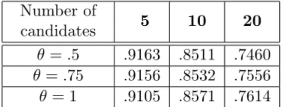
Table 3: Estimated probability of existence of a Condorcet winner in bi-normal profiles with 50 voters.
voters to X At some point, maybe after some other candidates have been tested, Y will be the challenger of X, and this Y will win. This implies that the process cannot stabilize for profiles with no Condorcet-winner. Recip-rocally, if a Condorcet winner exists, then the process will stabilize. This describes what is to happen if all dissatisfied voters simultaneously use the replacement tactic. It is more realistic to imagine that only some voters would do so. If we interpret the above process as a model of how intended votes adjust to anticipations (or pools), then it maybe more appropriate to think that the different voters adjust theirs votes in a sequential, rather than parallel manner. In any case, the argument remains that the replacement tactic, rather than the overstatement one, is efficient, and tends to turn the initial voting rule into a Condorcet-consistent one.
3.3.2 In a two-dimensional model
One may wonder to what extend the above arguments are restricted to the one-dimensional model. I therefore performed simulations4 using a two-dimension model, which may be closer to reality. In order to leave free the possible candidate configurations, which are more complex in two dimensions than in one, I choose at random the candidate positions. The positions of voters and candidates are all independently drawn from a bi-variate normal probability distribution, with standard deviation 1 on the first axis and θ ≤ 1 on the second one (without loss of generality).
To get an idea of the kind of profiles generated by this model, one can note that, with 50 independent voters, the probability of existence of a Condorcet-winner candidate is over 90% for 5 candidates, approximately 85% for 10 candidates, and approximately 75% for 20 candidates. More precisely, simulations on 10,000 random societies provide the figures reported in Table 3.
4
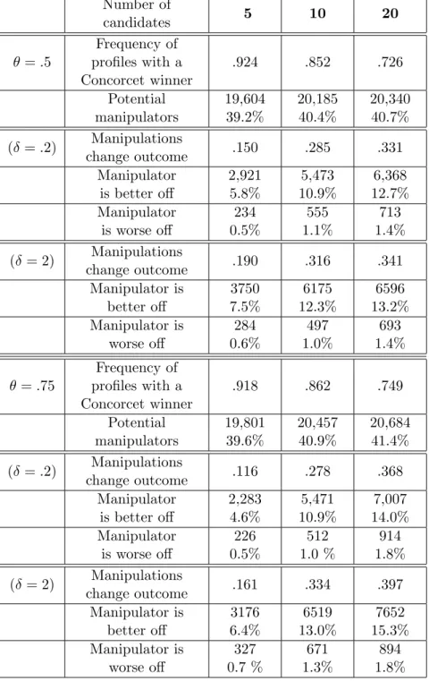
I now present the results of computer simulations with 50 voters and 10 candidates for θ = .75. Out of 1000 such societies, 862 exhibit a Condorcet winner. The Condorcet winner, when it exists is elected by the Hare pro-cess with frequency 467/862 = 54% On average, in the last round of the Hare elimination process, the winning candidate is supported by approx-imately 60% of the voters, so that when it comes to the “manipulation” studied in this paper, that is lowering the evaluation of the loser, there is on average 40% of potential manipulators, precisely 20, 457 out of a total of 50 × 1000 = 50, 000 voters. Let us suppose that these dissatisfied vot-ers modify their views by reporting a lower utility for the losing challenger. With the Euclidean spatial model which is used here, a typical distance be-tween a candidate and a voter isp2 ∗ (1 + (.75)2 ≈ 2.55. I first consider the
case of a slight penalty δ = .2 and then the case of a strong penalty δ = 2. With a slight penalty, the manipulation results in a different outcome in a fraction 278/1, 000 = .278 of the elections. See in Table 4 the fourth column which corresponds to 10 candidates, and the tenth row labeled “Ma-nipulation change outcome”, for θ = .75 and δ = .2. I obtain that, out of 20, 457 voters who distort their preference statements, 5, 471 end up being better off and 512 end up being worse off. Given the total number of vot-ers, these figures represent the respective frequencies indicated in the Table: 40.9%, 10.9% and 1.0%.
Of course, in most cases, the manipulation does not change the result of the election, but the “small understatement” manipulation, when it has an effect, is favorable for the manipulators at 90%. The frequency of election of the Condorcet winner raises from 54% to 569/862 = 66%.
An interesting point is the fact that the effect of the manipulation on the welfare of the whole electorate is also positive. In the 278 elections where the manipulation makes a difference, the sum of voters’ utility is increasing from −61.88 to −59.34 on average per election (figures not shown in the Table). Such will be also the case in all variants presented below.
Variations with the parameters can be seen in Table 4. With a strong penalty, the results are very similar, the manipulation has an effect only slightly more often (334 elections instead of 278), the number of satisfied manipulators slightly goes up (6, 519 instead of 5, 471) and the (small) num-ber of manipulators who regret the manipulation goes up accordingly (671 instead of 512).
The parameter θ is by definition between 0 and 1. The case θ = 0 would correspond to a uni-dimensional euclidean model. The case θ = .5 is intermediate between the case studied in the previous section and the case θ = .75. One can see from the Table that going from .75 to .5 does not
Number of candidates 5 10 20 θ = .5 Frequency of profiles with a Concorcet winner .924 .852 .726 Potential manipulators 19,604 39.2% 20,185 40.4% 20,340 40.7% (δ = .2) Manipulations change outcome .150 .285 .331 Manipulator is better off 2,921 5.8% 5,473 10.9% 6,368 12.7% Manipulator is worse off 234 0.5% 555 1.1% 713 1.4% (δ = 2) Manipulations change outcome .190 .316 .341 Manipulator is better off 3750 7.5% 6175 12.3% 6596 13.2% Manipulator is worse off 284 0.6% 497 1.0% 693 1.4% θ = .75 Frequency of profiles with a Concorcet winner .918 .862 .749 Potential manipulators 19,801 39.6% 20,457 40.9% 20,684 41.4% (δ = .2) Manipulations change outcome .116 .278 .368 Manipulator is better off 2,283 4.6% 5,471 10.9% 7,007 14.0% Manipulator is worse off 226 0.5% 512 1.0 % 914 1.8% (δ = 2) Manipulations change outcome .161 .334 .397 Manipulator is better off 3176 6.4% 6519 13.0% 7652 15.3% Manipulator is worse off 327 0.7 % 671 1.3% 894 1.8% Table 4: Simulation results for bi-normal profiles with 50 voters.
change much the results.
The most important parameter is the number of candidates. The ma-nipulations under consideration change the outcome more often when the number of candidates is large, as can be seen by reading the lines “Manipula-tions change outcome” in Table 4. Intuitively, it seems that the manipulation should work more often in cases where there are no Condorcet candidates. Therefore the observation may be linked to the fact that the Condorcet win-ner frequency decreases when the umber of candidates increases. Remark however that, with 50 voters and up to 20 candidates, one remains far away from theoretical continuous models that predict emptiness of the core; in fact the probability of existence of a Condorcet winner remains, in these finite models, above .7. In any case, the simulations show that the phe-nomenon highlighted in this paper is not restricted to the one-dimensional model.
4
Conclusion
It is often said that the systems of transferable votes like the Alternative Vote are resistant to manipulation. Analytical arguments put forth in favor of this thesis are of two kinds but can be phrased in the same game-theoretical setting: an n-player game, where n is the number of voters, in which a player is looking for its optimal ballot choice knowing exactly the other voters choices (so that the player knows when his personal vote will make a difference, at any point in the process of elimination).5
First the Computer Science literature has scrutinized the complexity of finding optimal responses in AV games and found that any algorithm designed to perform such a task would necessarily be very slow in some cases (Bartholdi & Orlin 1991). But these kind of results are obtained under worst-case analysis and that may be a too extreme stand, as to the study of voting rules (Walsh 2010). The perspective adopted here is quite different: even if it is very difficult to compute a best response, it may be relatively easy to find a response simply better than the sincere one.
Moreover following the game-theoretical classical model, the social choice and welfare literature usually considers manipulation as one and only voter changing her vote (Aleskerov & Kurbanov 1999). But in practice, in large elections, voting strategies, if any, are followed by several voters simulta-neously. Therefore in order to study the manipulability of voting rules for political elections, it is probably more realistic to imagine, that some
26 25 15 10 23 1
a b c c d d
c c d d a b
b d a b c a
d a b a b c
Table 5: A preference profile
tion of the electorate engage in one tactic or the other, as was done in this paper.
The remark made in this paper about AV invites to deepen the notion of correct voting for multi-candidate elections. Lau & Redlawsk (1997) defined correct voting as the vote for the candidate or party that the voter would have cast under full information. This definition is operational in the specific US context (Lau et al. 2008) but preferential voting like the Alternative Vote raises new problems. In that case, under full information, in particular as concern the chances of the various candidates, the voter may wish to cast a ballot which takes the form of a ranking of candidates and is different from her own preference ranking. Whether this should be labeled as “correct” voting or not is a matter of definition, but reading word for word the usual definition as “the vote that the voter would cast under full information” leads to consider as “correct” a vote that reflects the citizen’s true preferences in a distorted way.
A
Appendix
A.1 A successful “overstating” manipulation under AV
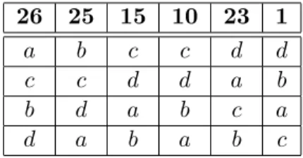
There are 100 voters, whose preference profile is provided in Table 5. The first collum states that 26 voters rank a first, c second, b third, and d last.
At such a profile, with the Hare system of elimination, d is eliminated first, with 23 transfers to a and one transfer to d. Then c is eliminated second but these votes are not transferred to d but to a and b. In the last round, a wins against b by 64 votes against 36.
Suppose now that the 10 voters with preference c > d > b > a overstate their preferences between a and b and put b at their first position. They thus announce b > c > d > a and the new profile is the one in Table 6.
In that case c is eliminated first, giving votes to d. Then a is eliminated second, and b wins against d in the last round by a 61 − 39 margin.
26 35 15 23 1
a b c d d
c c d a b
b d a c a
d a b b c
Table 6: A modified preference profile
References
[1] Fuad Aleskerov and Eldeniz Kubanov (1999) “Degree of manipulabil-ity of social choice procedures”. In S.Aliprantis, A.Alkan, N.Yannelis (Eds.), Studies in Economic Theory, Vol.8, Current Trends in Eco-nomics: Theory and Applications (pp. 13—28). Berlin: Springer. [2] Parimal Bag, Hamid Sabourian, and Eyal Winter (2009) “Multi-stage
voting, sequential elimination and Condorcet consistency”. Journal of Economic Theory 144: 1278—1299.
[3] Larry M. Bartels (1988) Presidential Primaries and the Dynamics of Public Choice. Princeton: Princeton University Press.
[4] John J. Bartholdi III and James B. Orlin (1991) “Single Transferable Vote Resists Strategic Voting” Social Choice and Welfare 8(4): 341— 354.
[5] Shaun Bowler and Bernard Grofman (eds.) (2000) Elections in Aus-tralia, Ireland, and Malta under the Single Transferable Vote. Ann Ar-bor: The University of MIchigan Press.
[6] John R. Chamberlin (1985) “An investigation into the relative manip-ulabiliy of four voting systems” Behavioral Science 30: 195—203. [7] Clyde H. Coombs (1964) Theory of Data. New York: John Wiley &
Sons.
[8] Gideon Doron and Richard Kronick (1977) “Single Transferable Vote: an example of a perverse social choice function” American Journal of Political Science 21: 303—311.
[9] David M. Farrell (2001) Electoral Systems: A comparative Introduction. London: Palgrave.
[10] David M. Farrell and Ian McAllister (2006) The Australian Electoral System: Origins, Variations, and Consequences. Sydney: University of New South Wales Press.
[11] Pierre Favardin and Dominique Lepelley (2006) “Some Further Results on the Manipulability of Social Choice Rules” Social Choice and Wel-fare 26: 485—509.
[12] Dan S. Felsenthal and Nicolaus Tideman (2014) “Interacting double monotonicity failure with direction of impact under five voting meth-ods” Mathematical Social Sciences 67: 57—66.
[13] Robert Forstythe, Roger Myerson, Thomas Rietz and Roberto Weber (1993) “An experiment on coordination in multicandidate elections: the importance of polls and election histories” Social Choice and Welfare 10: 223—247.
[14] Robert Forstythe, Roger Myerson, Thomas Rietz and Roberto Weber (1996) “An experimental study of voting rules and polls in three-way elections” International Journal of Game Theory 25: 355—383. [15] James Green-Armytage (2014) “Strategic Voting and Nomination”
So-cial Choice and Welfare 42: 111—138.
[16] Bernard Grofman and Scott L. Felds (2004) “If you like the alternative vote (a. k. a. the instant runoff), then you ought to know about the Coombs rule” Electoral Studies 23: 641—659.
[17] Jean-Fran¸cois Laslier (2010) “In Silico voting experiments” (2010) in the Handbook on Approval Voting (J.-F. Laslier and R. Sanver, eds.) Heidelberg: Springer. Chapter 13, pp. 311—335.
[18] Richard R. Lau, David J. Andersen, and David P. Redlawsk (2008) “An Exploration of Correct Voting in Recent U.S. Presidential Elections” American Journal of Political Science, 52: 395—411.
[19] Richard R. Lau and David P. Redlawsk (1997) “Voting Correctly” American Political Science Review 91: 585—99.
[20] Arend Lijphart (1994) Electoral Systems and Party Systems: A Study of Twenty-Seven Democracies, 1945-1990. Oxford: Oxford University Press.
[21] Herv´e Moulin (1979) “Dominance solvable voting schemes” Economet-rica 47: 1337—1351.
[22] Shmuel Nitzan (1985) “The vulnarability of point-voting schemes to preference variation and strategic manipulation” Public Choice 47: 349—370.
[23] Mat´ıas N´u˜nez and Jean-Fran¸cois Laslier (2014) “Preference intensity representation: Strategic overstating in large elections” Social Choice and Welfare 42: 313—340.
[24] Hannu Nurmi (2006) Models of Political Economy. London: Routledge. [25] Nicolaus Tideman (2006) Collective Decisions and Voting: The
Poten-tial for Public Choice Ashgate Publishing.
[26] Karine Van der Straeten, Jean-Fran¸cois Laslier, Nicolas Sauger and Andr´e Blais (2010) “Sincere, strategic, and heuristic voting under four election rules” Social Choice and Welfare 35(3): 435—472.
[27] Karine Van der Straeten, Andr´e Blais and Jean-Fran¸cois Laslier (2015) “Patterns of strategic voting in run-off electionss”. In Voting Exper-iments, edited by A. Blais, J.-F. Laslier and K. Van der Straeten, Springer.
[28] Toby Walsh (2010) “Manipulability of Single Transferable Vote” Computational Foundations of Social Choice, Dagstuhl Sem-inar Proceedings 10101, edited by F. Brandt, V. Conitzer, L. A. Hemaspaandra, J.-F. Laslier, W. S. Zwicker. LZI (http://drops.dagstuhl.de/opus/volltexte/2010/2558).
[29] Andy White (2010). “Tactical voting isn’t a practical strategy in Alternative Vote elections” British Policy and Politics at LSE, http://blogs.lse.ac.uk/politicsandpolicy/archives/3915