Vol.9(2010) No.3,pp.276-284
Analytic Approximate Solutions to The Coupled Lotka-Volterra
Equations with Fractional Derivatives
Zoubir Dahmani
∗, Ahmed Anber, Yasmina Khati Bouraoui
Department of Mathematics, Faculty of Sciences, University of Mostaganem, Mostaganem 27000 Algeria.
(Received 6 June 2009, accepted 19 January 2010)
Abstract:
By introducing the fractional derivative in the sense of Caputo, we apply the Adomian decompo-sition method for the coupled Lotka-Volterra equations with time-and space-fractional derivative. As a result, numerical solutions are obtained in a form of rapidly convergent series with easily computable components. The behavior of Adomian solutions are shown graphically for some examples.Keywords:
Adomian method; caputo fractional derivative; coupled Lotka-Volterra equations1
Introduction
Since Adomian firstly proposed the decomposition method [4, 5] at the begin of 1980s, the algorithm has been widely used for obtaining analytic solutions of physically significant equations [6, 15, 25–30]. With this method, we can easily obtain approximate solutions in the form of a rapidly convergent infinite series with each term computed conveniently[1, 2, 8, 13]. As we all know, for the nonlinear equations with derivatives of integer order, many methods are used to derive ap-proximation solutions [3–5, 7, 11, 18, 23, 24]. However, for the fractional differential equations, there are only limited approaches, such as Laplace transform method [20], the Fourier transform method [16], the iteration method [22] and the operational method [19].
In recent years, considerable interest in fractional differential equations has been stimulated due to their numerous appli-cations in the area of physics and engineering [9, 14, 31], like phenomena in electromagnetic theory, acoustics, electro-chemistry and material science [10, 12, 20, 22, 31].
We introduce Caputo fractional derivative and apply the ADM to derive numerical solutions of the coupled Lotka-Volterra equations with time and space fractional derivatives:
{ 𝐷𝛼 𝑡𝑢 = ( 𝐷𝛽 𝑥𝑢 )2+ 𝑢𝑢 𝑥𝑥+ 𝑏1𝑢2+ 𝑎1𝑢 + 𝑐1𝑣 + ℎ1 𝐷𝛼 𝑡𝑣 = ( 𝐷𝛽 𝑥𝑣 )2 + 𝑣𝑣𝑥𝑥+ 𝑏2𝑣2+ 𝑎2𝑣 + 𝑐2𝑢 + ℎ2, (1.1)
where𝑎1, 𝑎2, 𝑏1, 𝑏2, 𝑐1, 𝑐2, ℎ1, ℎ2are arbitrary constants such that𝑏1𝑏2∕= 0 and 𝑐1𝑐2∕= 0. When𝛼 = 𝛽 = 1, the fractional equations reduce to the coupled Lotka–Volterra equations :
{
𝑢𝑡= (𝑢𝑢𝑥)𝑥+ 𝑢 (𝑎1+ 𝑏1𝑢) + 𝑐1𝑣 + ℎ1
𝑣𝑡= (𝑣𝑣𝑥)𝑥+ 𝑣 (𝑎2+ 𝑏2𝑣) + 𝑐2𝑢 + ℎ2. (1.2)
The paper is organized as follows: In Sec. II, some necessary details on the fractional calculus are provided. In Sec. III, the coupled Lotka-Volterra equations with time-and-space-fractional derivatives are studied with the Adomian method and figures are used to show the efficiency as well as the accuracy of the approximate results are achieved. Finally, conclusions are followed.
∗+Corresponding author. E-mail address: [email protected].
Copyright c⃝World Academic Press, World Academic Union IJNS.2010.06.15/347
2
Description of Fractional Calculus
There are several mathematical definitions about fractional derivative[20, 22]. Here, we adopt the two usually used definitions: the Caputo and its reverse operator Riemann-Liouville. That is because Caputo fractional derivative allows traditional initial condition assumption and boundary conditions. More details one can consults [20]. In the following, we will give the necessary notation and basic definitions.
Definition 1 A real valued function𝑓(𝑥), 𝑥 > 0 is said to be in the space 𝐶𝜇, 𝜇 ∈ 𝑅 if there exists a real number 𝑝 > 𝜇
such that𝑓(𝑥) = 𝑥𝑝𝑓1(𝑥) where 𝑓1(𝑥) ∈ 𝐶([0, ∞)).
Definition 2 A function𝑓(𝑥), 𝑥 > 0 is said to be in the space 𝐶𝜇𝑛, 𝑛 ∈ 𝑁, if 𝑓(𝑛)∈ 𝐶𝜇.
Definition 3 The Riemann-Liouville fractional integral operator of order𝛼 ≥ 0, for a function 𝑓 ∈ 𝐶𝜇, (𝜇 ≥ −1) is defined as 𝐽𝛼𝑓(𝑥) = 1 Γ(𝛼) ∫𝑥 0(𝑥 − 𝑡)𝛼−1𝑓(𝑡)𝑑𝑡; 𝛼 > 0, 𝑥 > 0 𝐽0𝑓(𝑥) = 𝑓(𝑥). (2.1)
For the convenience of establishing the results for the fractional Lotka-Volterra equations, we give the properties
𝐽𝛼𝐽𝛽𝑓(𝑥) = 𝐽𝛼+𝛽𝑓(𝑥) (2.2)
and
𝐽𝛼𝑥𝛽 = Γ(𝛽+1)
Γ(𝛼+𝛽+1)𝑥𝛼+𝛽. (2.3)
Definition 4 The fractional derivative of𝑓 ∈ 𝐶−1𝑛 in the Caputo’s sense is defined as
𝐷𝛼𝑓(𝑡) = { 1 Γ(𝑛−𝛼) ∫𝑡 0(𝑡 − 𝜏)𝑛−𝛼−1𝑓(𝑛)(𝜏)𝑑𝜏, 𝑛 − 1 < 𝛼 < 𝑛, 𝑛 ∈ 𝑁∗, 𝑑𝑛 𝑑𝑡𝑛𝑓(𝑡), 𝛼 = 𝑛. (2.4)
According to the Caputo’s derivative, we can easily obtain the following expressions:
𝐷𝛼𝐾 = 0; 𝐾 is a constant, (2.5) 𝐷𝛼𝑡𝛽= { Γ(𝛽+1) Γ(𝛽−𝛼+1)𝑡𝛽−𝛼, 𝛽 > 𝛼 − 1, 0, 𝛽 ≤ 𝛼 − 1. (2.6)
Details on Caputo’s derivative can be found in [20].
Remark 1 In this paper, we consider equations (1.1) with time-and space-fractional derivative. When𝛼 ∈ 𝑅+, we have: 𝐷𝛼 𝑡𝑢(𝑥, 𝑡) =∂ 𝛼𝑢(𝑥, 𝑡) ∂𝑡𝛼 = { 1 Γ(𝑛−𝛼) ∫𝑡 0(𝑡 − 𝜏)𝑛−𝛼−1 ∂ 𝑛𝑢(𝑥,𝜏) ∂𝜏𝑛 𝑑𝜏, 𝑛 − 1 < 𝛼 < 𝑛 ∂𝑛𝑢(𝑥,𝑡) ∂𝑡𝑛 , 𝛼 = 𝑛. (2.7)
The form of the space fractional derivative is similar to the above.
3
The Analysis of the ADM Method
Consider the coupled equations with time-and space-fractional derivatives Eq.(1.1). Take the initial condition as {
𝑢 (𝑥, 0) = 𝑓 (𝑥)
𝑣 (𝑥, 0) = 𝑔 (𝑥) . (3.1)
Applying the operator𝐽𝛼, the inverse of𝐷𝛼in (1.1) and using the initial condition (3.1), yields: ⎧ ⎨ ⎩ 𝑢(𝑥, 𝑡) = 𝑓 (𝑥) + 𝐽𝛼(𝑃 1(𝑢 (𝑥, 𝑡))) + 𝐽𝛼(𝑃2(𝑢 (𝑥, 𝑡))) + 𝑏1𝐽𝛼(𝑃3(𝑢 (𝑥, 𝑡))) +𝑎1𝐽𝛼(𝑢) + 𝑐1𝐽𝛼(𝑣) + 𝐽𝛼(ℎ1) , 𝑣(𝑥, 𝑡) = 𝑔 (𝑥) + 𝐽𝛼(𝑄 1(𝑢 (𝑥, 𝑡))) + 𝐽𝛼(𝑄2(𝑢 (𝑥, 𝑡))) + 𝑏1𝐽𝛼(𝑄3(𝑢 (𝑥, 𝑡))) +𝑎2𝐽𝛼(𝑣) + 𝑐2𝐽𝛼(𝑢) + 𝐽𝛼(ℎ2) , (3.2)
where𝑃1(𝑢 (𝑥, 𝑡)) = (𝐷𝛽𝑥𝑢)2, 𝑃2(𝑢 (𝑥, 𝑡)) = 𝑢𝑢𝑥𝑥, 𝑃3(𝑢 (𝑥, 𝑡)) = 𝑢2, 𝑄1(𝑣 (𝑥, 𝑡)) = (𝐷𝑥𝛽𝑣)2, 𝑄2(𝑣 (𝑥, 𝑡)) =
𝑣𝑣𝑥𝑥 and 𝑄3(𝑣 (𝑥, 𝑡)) = 𝑣2.
The solution of Eq.(1.1) is represented as infinite series like ⎧ ⎨ ⎩ 𝑢 (𝑥, 𝑡) = ∑∞ 𝑛=0𝑢𝑛(𝑥, 𝑡) , 𝑣 (𝑥, 𝑡) = ∑∞ 𝑛=0𝑣𝑛(𝑥, 𝑡) . (3.3)
The nonlinear operators𝑃1(𝑢) , 𝑃2(𝑢) , 𝑃3(𝑢) , 𝑄1(𝑣) , 𝑄2(𝑣) and 𝑄3(𝑣) are decomposed in these forms
𝑃1(𝑢) = ∞ ∑ 𝑛=0𝐴𝑛, 𝑄1(𝑣) = ∞ ∑ 𝑛=0𝐷𝑛, 𝑃2(𝑢) = ∞ ∑ 𝑛=0𝐵𝑛, 𝑄2(𝑣) = ∞ ∑ 𝑛=0𝐸𝑛, 𝑃3(𝑢) = ∞ ∑ 𝑛=0𝐶𝑛, 𝑄3(𝑣) = ∞ ∑ 𝑛=0𝐹𝑛, (3.4)
where𝐴𝑛, 𝐵𝑛, 𝐶𝑛, 𝐷𝑛, 𝐸𝑛 and 𝐹𝑛are the so-called Adomian polynomials and have the form
𝐴𝑛=𝑛!1 𝑑 𝑛 𝑑𝜆𝑛 [ 𝑃1 (∑∞ 𝑘=0𝜆 𝑘𝑢 𝑘 )] 𝜆=0 = 1 𝑛! 𝑑 𝑛 𝑑𝜆𝑛 [( 𝐷𝛽 𝑥 (∑∞ 𝑘=0𝜆 𝑘𝑢 𝑘 ))2] 𝜆=0 , 𝐵𝑛= 𝑛!1 𝑑𝜆𝑑𝑛𝑛 [ 𝑃2 (∑∞ 𝑘=0𝜆 𝑘𝑢 𝑘 )] 𝜆=0 = 1 𝑛! 𝑑 𝑛 𝑑𝜆𝑛 [(∑∞ 𝑘=0𝜆 𝑘𝑢 𝑘 ) (∑∞ 𝑘=0𝜆 𝑘𝑢 𝑘𝑥𝑥 )] 𝜆=0 , 𝐶𝑛= 𝑛!1 𝑑 𝑛 𝑑𝜆𝑛 [ 𝑃3 (∑∞ 𝑘=0𝜆 𝑘𝑢 𝑘 )] 𝜆=0 = 1 𝑛! 𝑑 𝑛 𝑑𝜆𝑛 [(∑∞ 𝑘=0𝜆 𝑘𝑣 𝑘 )2] 𝜆=0 , 𝐷𝑛= 𝑛!1 𝑑𝜆𝑑𝑛𝑛 [ 𝑄1 (∑∞ 𝑘=0𝜆 𝑘𝑣 𝑘 )] 𝜆=0 = 1 𝑛! 𝑑 𝑛 𝑑𝜆𝑛 [( 𝐷𝛽 𝑥 (∑∞ 𝑘=0𝜆 𝑘𝑣 𝑘 ))2] 𝜆=0 , 𝐸𝑛 =𝑛!1 𝑑𝜆𝑑𝑛𝑛 [ 𝑄2 (∑∞ 𝑘=0𝜆 𝑘𝑣𝑘 )] 𝜆=0 = 1 𝑛! 𝑑 𝑛 𝑑𝜆𝑛 [(∑∞ 𝑘=0𝜆 𝑘𝑣𝑘 ) (∑∞ 𝑘=0𝜆 𝑘𝑣𝑘𝑥𝑥 )] 𝜆=0 , 𝐹𝑛= 𝑛!1 𝑑𝜆𝑑𝑛𝑛 [ 𝑄3 (∑∞ 𝑘=0𝜆 𝑘𝑣 𝑘 )] 𝜆=0 = 1 𝑛! 𝑑 𝑛 𝑑𝜆𝑛 [(∑∞ 𝑘=0𝜆 𝑘𝑣 𝑘 )2] 𝜆=0 . (3.5)
We give the first four components of these polynomials:
𝐴0=(𝐷𝑥𝛽𝑢0)2, 𝐴1= 2(𝐷𝛽𝑥𝑢0) (𝐷𝛽𝑥𝑢1), 𝐴2= 2(𝐷𝛽𝑥𝑢0) (𝐷𝑥𝛽𝑢2)+(𝐷𝑥𝛽𝑢1)2,
𝐴3=(𝐷𝑥𝛽𝑢0) (𝐷𝛽𝑥𝑢3)+(𝐷𝛽𝑥𝑢1) (𝐷𝛽𝑥𝑢2). (3.6)
The first four components of𝐵𝑛are:
𝐵0= 𝑢0𝑢0𝑥𝑥, 𝐵1= 𝑢0𝑢1𝑥𝑥+ 𝑢1𝑢0𝑥𝑥, 𝐵2= 𝑢0𝑢2𝑥𝑥+ 𝑢1𝑢1𝑥𝑥+ 𝑢2𝑢0𝑥𝑥,
𝐵3= 𝑢0𝑢3𝑥𝑥+ 𝑢1𝑢2𝑥𝑥+ 𝑢2𝑢1𝑥𝑥+ 𝑢3𝑢0𝑥𝑥. (3.7)
The first four components of𝐶𝑛are given by:
𝐶0= (𝑢0)2, 𝐶1= 2𝑢0𝑢1, 𝐶2= 2𝑢0𝑢2+ (𝑢1)2, 𝐶3= 𝑢0𝑢3+ 𝑢1𝑢2. (3.8)
The first four components of𝐷𝑛are:
𝐷0=(𝐷𝛽𝑥𝑣0)2, 𝐷1= 2(𝐷𝛽𝑥𝑣0) (𝐷𝛽𝑥𝑣1), 𝐷2= 2(𝐷𝛽𝑥𝑣0) (𝐷𝛽𝑥𝑣2)+(𝐷𝑥𝛽𝑣1)2,
𝐷3=(𝐷𝛽𝑥𝑣0) (𝐷𝛽𝑥𝑣3)+(𝐷𝑥𝛽𝑣1) (𝐷𝑥𝛽𝑣2), (3.9)
and those of𝐸𝑛and𝐹𝑛are given by:
𝐸0= 𝑣0𝑣0𝑥𝑥, 𝐸1= 𝑣0𝑣1𝑥𝑥+ 𝑣1𝑣0𝑥𝑥, 𝐸2= 𝑣0𝑣2𝑥𝑥+ 𝑣1𝑣1𝑥𝑥+ 𝑣2𝑣0𝑥𝑥,
𝐹0= (𝑣0)2, 𝐹1= 2𝑣0𝑣1, 𝐹2= 2𝑣2𝑣0+ (𝑣1)2, 𝐹3= 𝑣0𝑣3+ 𝑣1𝑣2. (3.11)
Substituting the decomposition series (3.3) and (3.4) into Eq(1.1), yields the following recursive formula:
𝑢0(𝑥, 𝑡) = 𝑓 (𝑥) , 𝑣0(𝑥, 𝑡) = 𝑔 (𝑥) ,
𝑢𝑛+1(𝑥, 𝑡) = 𝐽𝛼(𝐴𝑛) + 𝐽𝛼(𝐵𝑛) + 𝑏1𝐽𝛼(𝐶𝑛) + 𝑎1𝐽𝛼(𝑢𝑛) + 𝑐1𝐽𝛼(𝑣𝑛) + 𝐽𝛼(ℎ1) ,
𝑣𝑛+1(𝑥, 𝑡) = 𝐽𝛼(𝐸𝑛) + 𝐽𝛼(𝐹𝑛) + 𝑏´𝑒𝐽𝛼(𝐺𝑛) + 𝑎2𝐽𝛼(𝑣𝑛) + 𝑐2𝐽𝛼(𝑢𝑛) + 𝐽𝛼(ℎ2) .
(3.12)
The Adomian decomposition method converges generally very quickly. Details on its converegence and the conver-gence speed can be found in [1, 2, 8, 13]. Here according to the above steps, we will derive the numerical solutions for the coupled Eq(1.1) in details.
3.1
Numerical Solutions of Time-Fractional Lotka-Volterra Equations
Consider the following form of the time-fractional equations {
𝐷𝛼
𝑡𝑢 = (𝑢𝑥)2+ 𝑢𝑢𝑥𝑥+ 𝑏1𝑢2+ 𝑎1𝑢 + 𝑐1𝑣 + ℎ1
𝐷𝛼
𝑡𝑣 = (𝑣𝑥)2+ 𝑣𝑣𝑥𝑥+ 𝑏2𝑣2+ 𝑎2𝑣 + 𝑐2𝑢 + ℎ2 , 0 < 𝛼 ≤ 1, (3.13)
with the initial conditions ⎧ ⎨ ⎩ 𝑢 (𝑥, 0) = 𝑓 (𝑥) = 2 𝑡0 − 6𝑐1+ ( 2 𝑡0 − 6𝑐1+ 2𝑐1 𝑏 ) cos(√𝑏 2𝑥 − 𝛽0 ) , 𝑣 (𝑥, 0) = 𝑔 (𝑥) = 2 𝑡0 − 6𝑐1+ 4𝑐1 𝑏 +∣𝑐𝑐11∣ ( 2 𝑡0 − 6𝑐1+ 2𝑐1 𝑏 ) sin(√𝑏 2𝑥 − 𝛽0 ) , (3.14)
where𝑎1, 𝑎2, 𝑏1, 𝑏2, 𝑐1, 𝑐2, ℎ1, ℎ2, 𝛽0and𝑡0are arbitrary constants such that,𝑏 = 𝑏1= 𝑏2> 0, 𝑎1= 3𝑐1, 𝑎2= 𝑎1−6𝑐1,
𝑐2= −𝑐1.
The exact solution of the system (3.13) for the special case𝛼 = 1 is ⎧ ⎨ ⎩ 𝑢 (𝑥, 𝑡) = 𝜑0(𝑡) ±(𝜑0(𝑡) +2𝑐𝑏1)cos (√ 𝑏 2𝑥 ∓ ∣𝑐1∣ 𝑡 − 𝛽0 ) , 𝑣 (𝑥, 𝑡) = 𝜑0(𝑡) +4𝑐𝑏1 ±∣𝑐𝑐11∣(𝜑0(𝑡) +2𝑐𝑏1)sin (√ 𝑏 2𝑥 ∓ ∣𝑐1∣ 𝑡 − 𝛽0 ) , (3.15) where 𝜑0(𝑡) =3𝑏1 { 2 𝑡0−𝑡− 6𝑐1; 𝑎1= 3𝑐1 ∣3𝑐1− 𝑎1∣ tanh ( ∣3𝑐1−𝑎1∣ 2 (𝑡0− 𝑡) ) − 𝑎1− 3𝑐1; 𝑎1∕= 3𝑐1,
𝑎1, 𝑎2, 𝑏1, 𝑏2, 𝑐1, 𝑐2, ℎ1, ℎ2, 𝛽0and𝑡0are arbitrary constants such that,𝑏 = 𝑏1 = 𝑏2> 0, 𝑎2 = 𝑎1− 6𝑐1, 𝑐2 = −𝑐1,
ℎ1=(2𝑐1𝑎1−6𝑐
2 1)
𝑏 andℎ2= ℎ1+4𝑐𝑏1 (3𝑐1− 𝑎1) .
In order to obtain numerical solution of Eq.(3.13), substituting the initial conditions (3.14) and using the Adomian polynomial (3.6)-(3.11) into the expression (3.12), we can compute the results. For simplicity, we only give the first few
terms of series: 𝑢0= 𝑓 (𝑥) , 𝑣0= 𝑔 (𝑥) , 𝑢1= 𝐽𝛼(𝐴0) + 𝐽𝛼(𝐵0) + 𝑏1𝐽𝛼(𝐶0) + 𝑎1𝐽𝛼(𝑢0) + 𝑐1𝐽𝛼(𝑣0) + 𝐽𝛼(ℎ1) = 𝐽𝛼((𝑢 0𝑥)2 ) + 𝐽𝛼(𝑢 0𝑢0𝑥𝑥) + 𝑏1𝐽𝛼 ( (𝑢0)2 ) + 𝑎1𝐽𝛼(𝑢0) + 𝑐1𝐽𝛼(𝑣0) + 𝐽𝛼(ℎ1) = 𝑓1Γ(𝛼+1)𝑡𝛼 , 𝑣1= 𝐽𝛼(𝐷0) + 𝐽𝛼(𝐸0) + 𝑏2𝐽𝛼(𝐹0) + 𝑎2𝐽𝛼(𝑣0) + 𝑐2𝐽𝛼(𝑢0) + 𝐽𝛼(ℎ2) = 𝐽𝛼((𝑣 0𝑥)2 ) + 𝐽𝛼(𝑣 0𝑣0𝑥𝑥) + 𝑏2𝐽𝛼 ( (𝑣0)2 ) + 𝑎2𝐽𝛼(𝑣0) + 𝑐2𝐽𝛼(𝑢0) + 𝐽𝛼(ℎ2) = 𝑔1Γ(𝛼+1)𝑡𝛼 , 𝑢2= 𝐽𝛼(𝐴1) + 𝐽𝛼(𝐵1) + 𝑏1𝐽𝛼(𝐶1) + 𝑎1𝐽𝛼(𝑢1) + 𝑐1𝐽𝛼(𝑣1) + 𝐽𝛼(ℎ1) = 𝐽𝛼(2𝑢 0𝑥𝑢1𝑥) + 𝐽𝛼(𝑢0𝑢1𝑥𝑥+ 𝑢1𝑢0𝑥𝑥) + 𝑏1𝐽𝛼(2𝑢0𝑢1) + 𝑎1𝐽𝛼(𝑢1) + 𝑐1𝐽𝛼(𝑣1) + 𝐽𝛼(ℎ1) = 𝑓2Γ(2𝛼+1)𝑡2𝛼 , 𝑣2= 𝐽𝛼(𝐷1) + 𝐽𝛼(𝐸1) + 𝑏2𝐽𝛼(𝐹1) + 𝑎2𝐽𝛼(𝑣1) + 𝑐2𝐽𝛼(𝑢1) + 𝐽𝛼(ℎ2) = 𝐽𝛼(2𝑣 0𝑥𝑣1𝑥) + 𝐽𝛼(𝑣0𝑣1𝑥𝑥+ 𝑣1𝑣0𝑥𝑥) + 𝑏2𝐽𝛼(2𝑣0𝑣1) + 𝑎2𝐽𝛼(𝑣1) + 𝑐2𝐽𝛼(𝑢1) + 𝐽𝛼(ℎ2) = 𝑔2Γ(2𝛼+1)𝑡2𝛼 , 𝑢3= 𝐽𝛼(𝐴2) + 𝐽𝛼(𝐵2) + 𝐽𝛼(𝐶2) + 𝑎1𝐽𝛼(𝑢2) + 𝑏1𝐽𝛼(𝑣2) + 𝐽𝛼(ℎ1) = 𝐽𝛼(2𝑢0𝑥𝑢2𝑥+ (𝑢1𝑥)2)+ 𝐽𝛼(𝑢0𝑢2𝑥𝑥+ 𝑢1𝑢1𝑥𝑥+ 𝑢2𝑢0𝑥𝑥) + 𝑏1𝐽𝛼(2𝑢0𝑢2+ (𝑢1)2) +𝑎1𝐽𝛼(𝑢2) + 𝑐1𝐽𝛼(𝑣2) + 𝐽𝛼(ℎ1) = 𝑓3Γ(3𝛼+1)𝑡3𝛼 , 𝑣3= 𝐽𝛼(𝐷2) + 𝐽𝛼(𝐸2) + 𝑏2𝐽𝛼(𝐹2) + 𝑎2𝐽𝛼(𝑣2) + 𝑐2𝐽𝛼(𝑢2) + 𝐽𝛼(ℎ2) = 𝐽𝛼(2𝑣 0𝑥𝑣2𝑥+ (𝑣1𝑥)2 ) + 𝐽𝛼(𝑣 0𝑣2𝑥𝑥+ 𝑣1𝑣1𝑥𝑥+ 𝑣2𝑣0𝑥𝑥) + 𝑏2𝐽𝛼 ( 2𝑣0𝑣2+ (𝑣1)2 ) +𝑎2𝐽𝛼(𝑣2) + 𝑐2𝐽𝛼(𝑢2) + 𝐽𝛼(ℎ2) = 𝑔3Γ(3𝛼+1)𝑡3𝛼 , (3.16) where 𝑓1 = 𝑓𝑥2+ 𝑓𝑓𝑥𝑥+ 𝑏1𝑓2+ 𝑎1𝑓 + 𝑐1𝑔 + ℎ1, 𝑔1 = 𝑔𝑥2+ 𝑔𝑔𝑥𝑥+ 𝑏2𝑔2+ 𝑎2𝑔 + 𝑐2𝑓 + ℎ2, 𝑓2 = 2𝑓𝑥𝑓1𝑥+ 𝑓𝑓1𝑥𝑥+ 𝑓1𝑓𝑥𝑥+ 2𝑏1𝑓𝑓1+ 𝑎1𝑓1+ 𝑐1𝑔1+ ℎ1, 𝑔2 = 2𝑔𝑥𝑔1𝑥+ 𝑔𝑔1𝑥𝑥+ 𝑔1𝑔𝑥𝑥+ 2𝑏2𝑔𝑔1+ 𝑎2𝑔1+ 𝑐2𝑓1+ ℎ2, 𝑓3 = 2𝑓𝑥𝑓2𝑥+ 𝑓1𝑥2 + 𝑓𝑓2𝑥𝑥+ 𝑓1𝑓1𝑥𝑥+ 𝑓2𝑓𝑥𝑥+ 𝑏1(2𝑓𝑓2+ 𝑓12 ) + 𝑎1𝑓2+ 𝑐1𝑔2+ ℎ1, 𝑔3 = 2𝑔𝑥𝑔2𝑥+ 𝑔1𝑥2 + 𝑔𝑔2𝑥𝑥+ 𝑔1𝑔1𝑥𝑥+ 𝑔2𝑔𝑥𝑥+ 𝑏2(2𝑔𝑔2+ 𝑔12 ) + 𝑎2𝑔2+ 𝑐2𝑓2+ ℎ2, (3.17)
and so on in the same manner, the rest of the components of the recursive formulas (3.12) are obtained. Then we have the numerical solution of Eq.(3.13) under the series form
𝑢 (𝑥, 𝑡) = 𝑓 (𝑥) + 𝑓1Γ(𝛼+1)𝑡𝛼 + 𝑓2Γ(2𝛼+1)𝑡2𝛼 + 𝑓3Γ(3𝛼+1)𝑡3𝛼 + ...
𝑣 (𝑥, 𝑡) = 𝑔 (𝑥) + 𝑔1Γ(𝛼+1)𝑡𝛼 + 𝑔2Γ(2𝛼+1)𝑡2𝛼 + 𝑔3Γ(3𝛼+1)𝑡3𝛼 + ...
(3.18)
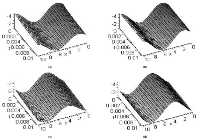
In order to verify the efficiency and accuracy of the proposed ADM method for the time-fractional Lotka-Voltera equations, we draw figures for the numerical solutions (3.18) with𝛼 = 1/2, as well as the exact solution (3.15) when
𝛼 = 1.
Remark 2 The accuracy of the numerical solution depend on how many terms we choose. In order to reduce the overall
errors, what we need is to add new terms to the decomposition series.
3.2
Numerical Solutions of Space-Fractional Lotka–Volterra Equations
Considering the operator form of the space-fractional equations { 𝑢𝑡=(𝐷𝑥𝛽𝑢 )2+ 𝑢𝑢 𝑥𝑥+ 𝑏1𝑢2+ 𝑎1𝑢 + 𝑐1𝑣 + ℎ1 𝑣𝑡=(𝐷𝛽𝑥𝑣 )2+ 𝑣𝑣 𝑥𝑥+ 𝑏2𝑣2+ 𝑎2𝑣 + 𝑐2𝑢 + ℎ2, (3.19)
with the initial conditions {
𝑢 (𝑥, 0) = 𝑓 (𝑥) = 𝑥2,
(a) (b)
(c) (d)
Figure 1: Representing time-fractional solutions of Eq.(3.13). In(a): the numerical solution u(x,t)-(3.18). In(b), the exact solution u(x,t)-(3.15) of Syst.(3.13). In(c): the numerical solution v(x,t)-(3.18). In(d), the exact solution v(x,t)-(3.15) of Eq.(3.13).𝑎1= 3/2; 𝑏1= 1; 𝑐1= 1/2; ℎ1= 1; 𝑎2= −3/2; 𝑏2= 1; 𝑐2= −1/2; ℎ2= 1; 𝛽0= 1; 𝑡0= 10; 𝛼 = 1/2;
In order to estimate the numerical solution of equations (3.19), substituting (3.3), (3.4) and using the initial conditions (3.20) into the expression (3.12), we get the Adomian solution. We give the first few terms of series:
𝑢0= 𝑓 (𝑥) , 𝑣0= 𝑔 (𝑥) , 𝑢1= 𝐽 (𝐴0) + 𝐽 (𝐵0) + 𝑏1𝐽 (𝐶0) + 𝑐1𝐽 (𝑣0) + 𝑎1𝐽 (𝑢0) + 𝐽 (ℎ1) = 𝐽((𝐷𝛽 𝑥𝑢0)2 ) + 𝐽 (𝑢0𝑢0𝑥𝑥) + 𝑏1𝐽 ( (𝑢0)2 ) + 𝑐1𝐽 (𝑣0) + 𝑎1𝐽 (𝑢0) + 𝐽 (ℎ1) =(𝑓2 1𝑥4−2𝛽+ 𝑏1𝑥4+ 𝑐1𝑥3+ (2 + 𝑎1) 𝑥2+ ℎ1)𝑡, 𝑣1= 𝐽 (𝐷0) + 𝐽 (𝐸0) + 𝑏2𝐽 (𝐹0) + 𝑐2𝐽 (𝑢0) + 𝑎2𝐽 (𝑣0) + 𝐽 (ℎ2) = 𝐽((𝐷𝛽 𝑥𝑣0)2 ) + 𝐽 (𝑣0𝑣0𝑥𝑥) + 𝑏2𝐽 ( (𝑣0)2 ) + 𝑐2𝐽 (𝑢0) + 𝑎2𝐽 (𝑣0) + 𝐽 (ℎ2) =(𝑔2 1𝑥6−2𝛽+ 𝑏2𝑥6+ 6𝑥4+ 𝑎2𝑥3+ 𝑐2𝑥2+ ℎ2)𝑡, 𝑢2= 𝐽 (𝐴1) + 𝐽 (𝐵1) + 𝑏1𝐽 (𝐶1) + 𝑐1𝐽 (𝑣1) + 𝑎1𝐽 (𝑢1) + 𝐽 (ℎ1) = 𝐽(2(𝐷𝛽 𝑥𝑢0) (𝐷𝑥𝛽𝑢1))+ 𝐽 (𝑢0𝑢1𝑥𝑥+ 𝑢1𝑢0𝑥𝑥) + 𝑏1𝐽 (2𝑢0𝑢1) + 𝑐1𝐽 (𝑣1) + 𝑎1𝐽 (𝑢1) + 𝐽 (ℎ1) = (𝑓2𝑥8−5𝛽+ 𝑓3𝑥8−3𝛽+ 𝑓4𝑥7−3𝛽+ 𝑓5𝑥6−3𝛽+ 𝑓6𝑥4−3𝛽+ 𝑓7𝑥6−2𝛽+ 𝑓8𝑥4−2𝛽+ 𝑓9𝑥2−2𝛽 +𝑓10𝑥6+ 𝑓11𝑥5+ 𝑓12𝑥4+ 𝑓13𝑥3+ 𝑓14𝑥2+ 𝑓15𝑥 + 𝑓16)𝑡22, 𝑣2= 𝐽 (𝐷1) + 𝐽 (𝐸1) + 𝑏2𝐽 (𝐹1) + 𝑐2𝐽 (𝑢1) + 𝑎2𝐽 (𝑣1) + 𝐽 (ℎ2) = 𝐽(2(𝐷𝛽 𝑥𝑣0) (𝐷𝑥𝛽𝑣1))+ 𝐽 (𝑣0𝑣1𝑥𝑥+ 𝑣1𝑣0𝑥𝑥) + 𝑏2𝐽 (2𝑣0𝑣1) + 𝑐2𝐽 (𝑢1) + 𝑎2𝐽 (𝑣1) + 𝐽 (ℎ2) . = (𝑔2𝑥9−4𝛽+ 𝑔3𝑥9−2𝛽+ 𝑔4𝑥8−2𝛽+ 𝑔5𝑥7−2𝛽+ 𝑔6𝑥6−2𝛽+ 𝑔7𝑥3−2𝛽+ 𝑔8𝑥4−2𝛽+ 𝑔9𝑥7 +𝑔10𝑥9+ 𝑔11𝑥5+ 𝑔12𝑥6+ 𝑔13𝑥4+ 𝑔14𝑥3+ 𝑔15𝑥2+ 𝑔16𝑥 + 𝑔17)𝑡22. (3.21)
where 𝑓 (𝑥) = 𝑥2, 𝑓 1= ( Γ(3) Γ(3−𝛽) ) , 𝑓2= 2𝑓12Γ(5−2𝛽)Γ(5−3𝛽), 𝑓3= 2𝑏1𝑓12Γ(5−𝛽)Γ(5) , 𝑓4= 2𝑐1𝑓12Γ(4−𝛽)Γ(4) , 𝑓5= 2 (2 + 𝑎1) 𝑓13, 𝑓6=(2𝑏1𝑓12+ 𝑐1𝑔21 ) , 𝑓7=((4 − 2𝛽) (3 − 2𝛽) 𝑓1+ 𝑎1𝑓12 ) , 𝑓8= (2 (4 − 2𝛽) (3 − 2𝛽) 𝑓1) , 𝑓9=(2𝑏21+ 𝑏2𝑐1), 𝑓10= (2𝑏1𝑐1) , 𝑓11= (12𝑏1+ 4𝑏1+ 2𝑏1𝑎1+ 6𝑐1+ 2𝑏1) , 𝑓12= (6𝑐1+ 𝑎2𝑐1+ 𝑎1𝑐1) , 𝑓13=(4𝑎1+ 24𝑏1+ 2𝑏1ℎ1+ 𝑐21+ 𝑎21+ 4 ) , 𝑓14= 12𝑐1, 𝑓15= 4𝑎1+ 𝑐1ℎ2+ 𝑎1ℎ1+ 8, 𝑔 (𝑥) = 𝑥3, 𝑔 1= ( Γ(4) Γ(4−𝛽) ) , 𝑔2= 2𝑔1Γ(7−2𝛽)Γ(7−3𝛽), 𝑔3= ( 2𝑏2𝑔1Γ(6−𝛽)Γ(6) + 2𝑏2𝑔21 ) , 𝑔4= ( 12𝑔1Γ(5−𝛽)Γ(5) ) , 𝑔5=(2𝑎2𝑔12+ 6𝑔12+ (6 − 2𝛽) (5 − 2𝛽) 𝑔12 ) , 𝑔6=(2𝑔2𝑐2𝑓1+ 𝑎2𝑔22 ) , 𝑔7= 𝑐2𝑓12, 𝑔8= 48𝑏2, 𝑔9= 2𝑏22, 𝑔10= (108 + 2𝑐2𝑏2) , 𝑔11= 3𝑎2𝑏2, 𝑔12= (18𝑎2+ 𝑐2𝑏2) , 𝑔13=(8𝑐2+ 2ℎ2𝑏2+ 𝑐1𝑐2+ 𝑎22 ) , 𝑔14= (2𝑐2+ 2𝑐2𝑎1) , 𝑔15= 6ℎ2, 𝑔16= ℎ1𝑐2+ 𝑎2ℎ2, (3.22)
Then we obtain a numerical solution of space-fractional equations (3.16) in series form ⎧ ⎨ ⎩ 𝑢 (𝑥, 𝑡) = 𝑓 (𝑥) +(𝑓2 1𝑥4−2𝛽+ 𝑏1𝑥4+ 𝑐1𝑥3+ (2 + 𝑎1) 𝑥2+ ℎ1)𝑡 + (𝑓2𝑥8−5𝛽 +𝑓3𝑥8−3𝛽+ 𝑓4𝑥7−3𝛽+ 𝑓5𝑥6−3𝛽+ 𝑓6𝑥6−2𝛽+ 𝑓7𝑥4−2𝛽+ 𝑓8𝑥2−2𝛽 +𝑓9𝑥6+ 𝑓10𝑥5+ 𝑓11𝑥4+ 𝑓12𝑥3+ 𝑓13𝑥2+ 𝑓14𝑥 + 𝑓15)𝑡22 + ... 𝑣 (𝑥, 𝑡) = 𝑔 (𝑥) +(𝑔2 1𝑥6−2𝛽+ 𝑏2𝑥6+ 6𝑥4+ 𝑎2𝑥3+ 𝑐2𝑥2+ ℎ2)𝑡 + (𝑔2𝑥9−4𝛽 +𝑔3𝑥9−2𝛽+ 𝑔4𝑥8−2𝛽+ 𝑔5𝑥7−2𝛽+ 𝑔6𝑥6−2𝛽+ 𝑔7𝑥4−2𝛽+ 𝑔8𝑥7+ 𝑔9𝑥9 +𝑔10𝑥5+ 𝑔11𝑥6+ 𝑔12𝑥4+ 𝑔13𝑥3+ 𝑔14𝑥2+ 𝑔15𝑥 + 𝑔16)𝑡22 + ... (3.23)
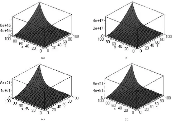
The figures below show the numerical solution (3.23) for the space-fractional Lotka-Voltera Eq.(3.19) with𝛼 = 𝛽 = 1/2 as well as the numerical solution of Eq.(3.19) with 𝛼 = 𝛽 = 1.
(a) (b)
(c) (d)
Figure 2: Representing space-fractional solutions of Eq.(3.19). In(a) and (c) solution obtained by the Adomian method of u(x,t) and v(x,t) for𝛽= 1 . In(b) and (d), solution obtained by the Adomian method of u(x,t) and v(x,t) for 𝛽= 1 /2 .
4
Conclusion
In this paper, the ADM has been successfully applied to derive explicit numerical solutions for the coupled Lotka-Volterra equations with time-and-space fractional derivatives. The above procedure shows that the ADM method is efficient and powerful in solving wide classes of equations in particular evolution fractional order equations.
References
[1] K. Abbaoui and Y. Cherruault. Convergence of Adomian’s method applied to differnetial equations. Comput. Math.
Appl., 28(5):(1994),103-109.
[2] K. Abbaoui and Y. Cherruault. New ideas for proving convergence of decomposition method. Comput. Math. Appl., 29:(1995),103-108.
[3] M. J. Ablowitz and P.A. Clarkson. Solitons, nonlinear evolution equations and inverse scatting. Cambridge
Univer-sity Press, New York (1991).
[4] G. Adomian. Nonlinear stochastic Systems theory and applications to Physics. Kluwer Academic Publishers,
Dor-drecht,(1989).
[5] G. Adomian. Solving frontier problems of Physics: The decomposition method. Kluwer Academic Publishers,
Boston,(1994).
[6] E. BABOBLIAN, A. DAVARI, Numerical implementation of Adomian decomposition method for linear Volterra integral equation of the second kind, Appl. Math. Comput., 165 :(2005), 223-227.
[7] Y. Chen and Y. Z. Yan. Weierstrass semi rational expansion method and new doubly periodic solutions of the gener-alized Hirota-Satsuma coupled KdV system. Appl. Math. Comput., 177:(2006),85-91.
[8] Y. Cherruault.Convergence of Adomian’s method.Kybernetes, 18:(1989),31-38.
[9] V. Daftardar-Gejji, H. Jafari. Adomian decomposition: a tool for solving a system of fractional differential equations.
J. Math. Anal. Appl., 301:(2005), 508-518.
[10] Z. Dahmani, M. M. Mesmoudi and R. Bebbouchi. The foam-drainage equation with time and space fractional deriva-tive solved by the ADM method. E. J. Qualitaderiva-tive Theory of Diff. Equ., 30:(2008),1-10.
[11] E. Fan. Extended tanh function method and its applications to nonlinear equations. Phys. Lett. A.,277:( 2000), 212-218.
[12] J. H. He. Some applications of nonlinear fractional differential equations and their approximations. Bull. Sci. Techno., 15(2):(1999),86-90.
[13] N. Himoun, K. Abbaoui and Y. Cherruault. New results of convergence of Adomian’s method. Kybernetes, 28(4-5):(1999),423-429.
[14] H. Jafari and V. Daftardar-Gejji. Solving a system of nonlinear fractional differential equations using Adomian decomposition. J. Comput. Appl. Math., 196:(2006),644-651.
[15] D. Kaya and S. M. El Sayad. A numerical implementation of the decomplosition method for the Lienard equation.
Appl. Math. Comput., 171:(2005),1095-1103.
[16] S. Kemple and H. Beyer. Global and causal solutions of fractional differential equations in : Transform Method and Special Functions. Varna96, Proceding of the 2nd International Workshop (SCTP), Singapore,(1997).
[17] B. A. Kupershmidt. Mathematics of dispersive water waves. Communications in Mathematical Physics, 99:( 1995),51-73.
[18] Y. Luchko and R. Gorenflo. The initial value problem for some fractional differential equations with the Caputo derivaitve. Preprint Series A 08-98, Fachbereich Mathematik und Informatik, Freie Universitat Berlin,(1998). [19] Y. Luchko and H. M. Srivastava. The exact solutions of certain differential equations of fractional order by using
operational calculus. Comput. Math. Appl., 29:(1995),73-85 .
[20] I. Podlubny. Fractional Differential Equations. Academic Press, San Diego.,(1999).
[21] M. Rafei and H. Daniali. Application of the variational iteration method to the Whitham–Broer–Kaup equations.
Appl. Math. Comput., (2006).
[22] G. Samko, A. A. Kilbas and O. I. Marichev. Fractional integral and derivative: Theory and Applications. Gordon
and Breach, Yverdon,(1993).
[23] S. Momani and Z. Odibat. Numerical approach to differential equations of fractional order. J. Comput. Appl. Math., 207:(2007),96-110.
[24] Q. Wang. Numerical solutions for fractional KdV-Burgers equation by Adomian decomposition method. Appl. Math.
[25] A. M. Wazwaz. A new approch to the nonlinear advection problem. Appl. Math. Comput., 72:(1995),175-181. [26] A. M. Wazwaz. A reliable modification of Adomian decomposition method. Appl. Math. Comput., 102:(
1999),77-86.
[27] A. M. Wazwaz. A new algorithm for calculating Adomian polynomials for nonlinear operators. Appl. Math. Comput., 111:(2000), 53-69.
[28] A. M. Wazwaz. A computational approach to solitons of the Kadomtsev-Petviashvili equation. Appl. Math. Comput., 123:(2001),205-217.
[29] A. M. Wazwaz. Partial differential equations: Methods and Applications. Balkema Publishers. The
Nether-lands,(2002).
[30] A. M. Wazwaz, A. Georguis. An analytic study of Fisher’s equations by using Adomian decomposition method.
Appl. Math. Comput., 154:(2004),609-620.