Renormalized solutions to a class of quasilinear elliptic problems with weak data : existence, uniqueness and homogenization

HAL Id: tel-03228329

https://tel.archives-ouvertes.fr/tel-03228329

Submitted on 18 May 2021

HAL is a multi-disciplinary open access

archive for the deposit and dissemination of sci-entific research documents, whether they are pub-lished or not. The documents may come from teaching and research institutions in France or abroad, or from public or private research centers.

L’archive ouverte pluridisciplinaire HAL, est destinée au dépôt et à la diffusion de documents scientifiques de niveau recherche, publiés ou non, émanant des établissements d’enseignement et de recherche français ou étrangers, des laboratoires publics ou privés.

Renormalized solutions to a class of quasilinear elliptic

problems with weak data : existence, uniqueness and

homogenization

Rheadel Fulgencio

To cite this version:

Rheadel Fulgencio. Renormalized solutions to a class of quasilinear elliptic problems with weak data : existence, uniqueness and homogenization. Analysis of PDEs [math.AP]. Normandie Université, 2021. English. �NNT : 2021NORMR010�. �tel-03228329�

“You must forge your own path for it to mean anything.” -Rick Riordan, The Lost Hero

Abstract

In this thesis, we study a class of quasilinear elliptic equations posed in a two-component domain with an L1 _{data and its asymptotic analysis. More}

precisely, we consider a two-component domain, denoted by Ω, which can be written as the disjoint union Ω = Ω1 [ Ω2 [ Γ, where the open sets Ω1

and Ω2 are the two components of Ω, and Γ is the interface between these

components. We study the following quasilinear elliptic problem posed in Ω: 8 > > > > > > < > > > > > > : div(B(x, u1)ru1) = f in Ω1, div(B(x, u2)ru2) = f in Ω2, (B(x, u1)ru1)⌫1 = (B(x, u2)ru2)⌫1 on Γ, (B(x, u1)ru1)⌫1 = h(x)(u1 u2) on Γ, u1 = 0 on @Ω,

where ⌫1 is the unit outward normal to Ω1, f is an L1 function, and B is

a coercive matrix field which has a restricted growth assumption (B(x, r) is bounded on any compact set of R).

The first part of this thesis is dedicated to existence and uniqueness re-sults for this problem in the framework of renormalized solutions, which was introduced by R.J. DiPerna and P.L. Lions.

In the second part, we study the corresponding homogenization problem for a two-component domain with a (disconnected) periodic second com-ponent by combining the notion of renormalized solutions and the periodic unfolding method, introduced D. Cioranescu, A. Damlamian and G. Griso. It has been successively adapted to two-component domains by P. Donato, K.H. Le Nguyen, and R. Tardieu.

In order to obtain a uniqueness result for the homogenized problem, we study the properties of the corresponding cell problem. In particular, we show that if the matrix field in the cell problem, denoted A(y, t), is local Lipschitz-continuous with respect to t, then the resulting homogenized matrix A0 _keeps

this property. This uniqueness result ensures that the convergences obtained in the homogenization process hold for the whole sequence of the periodicity parameter (and not only a subsequence).

Résumé

Dans cette thèse, nous étudions une classe de problèmes elliptiques quasi-linéaires posés dans un domaine à deux composantes avec une donnée L1 _et

son analyse asymptotique. Plus précisement, on considère un domaine Ω, que l’on écrit comme une réunion disjointe Ω = Ω1[ Ω2[ Γ, où les ensembles

ouverts Ω1 et Ω2 sont les deux composantes de Ω, et Γ est l’interface entre

les composantes. Nous étudions le problème elliptique quasi-linéaire suivant posé dans Ω : 8 > > > > > > < > > > > > > :

div(B(x, u1)ru1) = f dans Ω1,

div(B(x, u2)ru2) = f dans Ω2,

(B(x, u1)ru1)⌫1 = (B(x, u2)ru2)⌫1 sur Γ,

(B(x, u1)ru1)⌫1 = h(x)(u1 u2) sur Γ,

u1 = 0 sur @Ω,

où ⌫1 est le vecteur normal unitaire extérieur à Ω1, f 2 L1(Ω) et B est une

matrice coercitive qui vérifie une hypothèse assez générale (B(x, r) n’est pas uniformément borné mais borné sur tout ensemble compact de R).

La première partie de cette thèse est donc dédiée à des résultats d’existence et d’unicité de ce problème dans le cadre des solutions renormalisées, qui a été introduit par R.J. DiPerna et P.L. Lions.

Dans la deuxième partie, nous étudions l’homogénéisation d’un problème du même type, posé dans un domaine à deux composantes dont la deuxième est une réunion périodique d’ensembles déconnectés, en mélangeant le notion des solution renormalisées et la méthode de l’éclatement périodique. Cette méthode a été introduite par D. Cioranescu, A. Damlamian and G. Griso et adaptée aux domaines à deux composantes par P. Donato, K.H. Le Nguyen, et R. Tardieu.

Pour obtenir un résultat d’unicité pour le problème homogénéisé qui puisse assurer que les convergences obtenues sont valables pour toute la suite du paramètre de périodicité (et non pas à une sous-suite près), nous étudions les propriétés du problème périodique correpondant, posé dans la cellule de référence. En particulier, nous démontrons que si la matrice A(y, t) du prob-lème dans la cellule de référence est localement lipschitzienne par rapport à t, alors la matrice homogénéisée résultante A0_{(t) garde cette propriété.}

Acknowledgments

I would like to express my sincere appreciation to the people and organiza-tions who made this incredible journey possible.

First and foremost, to my PhD thesis supervisors, Prof. Patrizia Donato and Prof. Olivier Guibé, I owe you my deepest gratitude. You are the best supervisors that I could hope for. Discussing with you and learning from your vast knowledge have been great experiences for me. Thank you for being patient and supportive of me during the past 3 years. I know that this is not the end, but just the start of more research collaborations.

To the members of the jury, Prof. Juan Casado-Díaz, Prof. Nicolas Forcadel, Prof. Editha Jose, Prof. Jose Ernie Lope, and Prof. Anna Mercaldo, thank you for taking the time to read my thesis and to attend my defense.

To the members of my follow-up committee, Prof. Forcadel and Prof. Lope, thank you for making time for the yearly meeting to check on my progress and to make sure that everything is fine. I specially thank Prof. Lope, who has been guiding me since my undergraduate years, as both my undergraduate and masters thesis adviser.

To LMRS of University of Rouen Normandy, thank you for your warm wel-come and for being accommodating to my needs. I would also like thank the people I met in the lab, everyone has been very nice to me. Thank you for not letting me feel alone during my stay.

To the Institute of Mathematics of UP Diliman, thank you for letting me have this chance to pursue my PhD in France. I give my special regards to Prof. Marian Roque, who introduced me to Prof. Donato.

To CHED and Embassy of France to the Philippines and Micronesia, thank you for granting me the CHED-PhilFrance scholarship and giving me the means to have this golden opportunity.

To my friends, thank you for always being supportive. Special mention to Arrianne and Thirdie, with whom I shared the same experiences of being a Filipino student in a French environment. You made the hard and confusing times bearable.

To my family, Mama, Papa, Adrian, and AM, thank you for everything. You have been and always will be my inspiration. Thank you for being the best family there is.

Finally, to Aaron, I can’t believe we made it. Thank you for not giving up when I almost did. I’ll see you soon.

Contents

Résumé de la thèse 1

1 Introduction 19

1.1 Renormalized solutions . . . 20

1.1.1 A model case . . . 21

1.1.2 Our renormalized solution results . . . 31

1.2 Homogenization theory . . . 39

1.2.1 Multiple-scales method . . . 43

1.2.2 Tartar’s method of oscillating test functions . . . 45

1.2.3 Two-scale convergence method . . . 47

1.2.4 The periodic unfolding method . . . 50

1.2.5 Our homogenization results . . . 56

I

Existence and uniqueness results

63

2 Quasilinear elliptic problems in a two-component domain with L1 _{data 65} 2.1 Introduction . . . 65

2.2 Assumptions and Definitions . . . 67

2.3 Existence Results . . . 75

3 Uniqueness for quasilinear elliptic problems in a two-component domain with L1 _{data 89} 3.1 Introduction . . . 89

3.2 Assumptions and Definitions . . . 90

3.3 Preliminary Results . . . 94

II

Homogenization results

117

4 Some properties of an elliptic periodic problem with an in-terfacial resistance 119

4.1 Introduction . . . 119

4.2 Statement of the problem . . . 123

4.3 A Meyers type estimate . . . 126

4.4 The rescaled problem . . . 131

4.5 Further properties for a quasilinear case . . . 135

4.6 Boundedness of the solution . . . 140

5 Homogenization results for quasilinear elliptic problems in a two-component domain with L1 _{data 143} 5.1 Introduction . . . 143

5.2 Preliminaries and Position of the Problem . . . 147

5.3 A priori estimates . . . 155

5.4 Homogenization Results . . . 166

Perspectives 189

Résumé de la thèse

Dans cette thèse, nous étudions une classe de problèmes elliptiques quasi-linéaires posés dans un domaine à deux composantes avec une donnée L1 _et

nous en faisons l’analyse asymptotique dans un domaine périodique à deux composantes. Plus précisement, on considère un domaine Ω, que l’on écrit comme une réunion disjointe

Ω = Ω1[ Ω2[ Γ,

où les ensembles ouverts Ω1 et Ω2 sont les deux composantes de Ω, et Γ

est l’interface entre les composantes. Nous étudions le problème elliptique quasi-linéaire suivant posé dans Ω :

8 > > > > > > < > > > > > > :

div(B(x, u1)ru1) = f dans Ω1,

div(B(x, u2)ru2) = f dans Ω2,

(B(x, u1)ru1)⌫1 = (B(x, u2)ru2)⌫1 sur Γ,

(B(x, u1)ru1)⌫1 = h(x)(u1 u2) sur Γ,

u1 = 0 sur @Ω,

(1) où ⌫1 est le vecteur normal unitaire extérieur à Ω1, f 2 L1(Ω) et B est une

matrice coercitive qui vérifie une hypothèse assez générale (B(x, r) n’est pas uniformément borné mais borné sur tout ensemble compact de R).

Observons que sous les hypothèses précédentes sur f et B nous ne pouvons pas, en général, obtenir l’existence d’une solution faible. Même si f 2 L2_(Ω)

sans hypothèse de bornitude sur B(x, r) par rapport à r, on ne sait pas démontrer en général l’existence d’une solution faible (de même si B est borné et f 2 L1_(Ω)).

Rappelons que le problème

div(A(x, u)ru) = f

avec des conditions de Dirichlet sur le bord, si A(x, r) est bornée, elliptique et f appartient à L1_{(Ω) (ou même est une mesure bornée de Radon), il existe}

d’apres Boccardo-Gallouët [18] une solution au sens des distributions (et ces résultats sont valable pour une classe plus général d’opérateurs non linéaires à croissance p). Les auteurs démontrent que u 2 W1,q

0 (Ω), 81 < q < N N 1 et verifie _Z Ω A(x)rur' dx = Z Ω f ' dx, 8' 2 C₀1(Ω).

Cependant, cette solution au sens des distributions ne peut pas avoir, en général, une énergie finie, au sens où u /2 H1

0(Ω). De plus même dans le

cas linéaire, c’est-à-dire A(x, r) = A(x), la solution au sens des distributions n’est pas unique en général d’apres le contre exemple de Serrin [78] (voir aussi [76]).

Pour pallier cet inconvénient, plusieurs notions de solutions ont été dévelop-pées : solutions entropiques (voir [10]), SOLA (solutions obtenues comme limite d’approximation, voir [37]) et solutions renormalisées.

Pour mener à bien notre étude sur le problème (1) (existence, unicité, analyse asymptotique), nous avons besoin d’une notion de solution qui per-met des résultats d’unicité et de stabilité. Nous utiliserons dans cette thèse la notion de solution renormalisée.

La notion de solution renormalisée a été introduite dans [39] par R.J. DiPerna et P.L. Lions pour des équations du premier ordre. Elle a été développée ensuite par F. Murat dans [71], par P.L. Lions et F. Murat dans [63] pour des équations elliptiques avec conditions de Dirichlet et données L1_{, puis par G. Dal Maso et al. dans [36] pour des équations elliptiques}

avec données mesures. La plupart des travaux concernant le développement des solutions renormalisées traite de problèmes elliptiques (ou paraboliques) à données L1 _{et avec des conditions de Dirichlet, mais plus rarement le cas}

d’autres conditions sur le bord (citons [13] pour des conditions de Neumann, [59] pour un domaine perforé). L’existence et l’unicité d’une solution renor-malisée ont été étudiées pour des domaines perforés dans [59], avec une condi-tion de Fourier sur le bord des trous, mais, à notre connaissance les équacondi-tions de type (1) avec donnée L1 _{et saut à l’interface n’ont pas été abordées dans}

la littérature.

La première partie de cette thèse est donc dédiée à des résultats d’existence et d’unicité pour la solution du problème (1). Nous avons donné d’abord une définition appropriée de solution renormalisée du problème. Cette définition, ainsi que le résultat d’existence, sont présentés dans le chapitre 2. L’unicité de cette solution est démontrée dans le chapitre 3, où une hypothése supplé-mentaire de lipschitzianité locale pour la matrice B est nécessaire.

Dans la deuxième partie, nous étudions l’homogénéisation d’un problème du même type, posé dans un domaine à deux composantes dont la deuxième

est une réunion périodique d’ensembles déconnectés, qui est présentée dans le chapitre 5. Dans ce chapitre, nous identifions d’abord, en utilisant les estima-tions a priori obtenues dans la première partie, le problème éclaté (théorème 12). Nous obtenons ensuite le problème homogénéisé dans Ω (théorème 13). Pour y parvenir, nous utilisons la méthode de l’éclatement périodique, qui a été introduite dans [31] pour des domaines fixes et dans [29] pour des domaines perforées. Elle a été étendue successivement au cas de domaines à deux composantes dans [46] et [45] (pour une présentation générale nous renvoyons au livre récent [32]).

Pour obtenir un résultat d’unicité pour le problème homogénéisé qui puisse assurer que les convergences obtenues sont valables pour toute la suite du paramètre de périodicité (et non pas à une sous-suite près), nous étudions dans le chapitre 4 les propriétés du problème périodique correpondant, posé dans la cellule de référence (voir (10)). En particulier, nous démontrons que si la matrice A(y, t) du problème dans la cellule de référence est localement lipschitzienne par rapport à t, alors la matrice homogénéisée résultante A0_(t)

(voir (12)) garde cette propriété. Les résultats obtenus dans cette thèse sont présentés ci-dessous en détails.

Le chapitre 1 est dédié à l’introduction de la thèse en anglais.

Partie I

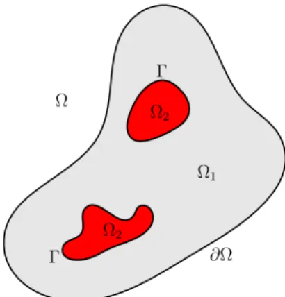
Dans cette partie, nous étudions l’existence et l’unicité de la solution renor-malisée de (1). On définit d’abord le domaine à deux composantes Ω, qui est un ensemble ouvert borné connexe de RN _{de frontière @Ω. Nous}

décom-posons le domaine comme la réunion disjointe Ω = Ω1[ Ω2[ Γ, où Ω2 est un

ensemble ouvert tel que Ω2 ⇢ Ω de frontière lipschitzienne Γ, et Ω1 = Ω \ Ω2

(voir figure 1). Ω Ω2 Γ Ω2 Γ Ω1 ∂Ω

lim n!1 1 n Z Γ (u1 u2)(Tn(u1) Tn(u2)) d = 0; (3b)

et pour tout S1, S2 2 C1(R) (ou S1, S2 2 W1,1(R)) à support compact, u

satisfait Z Ω1 S1(u1)B(x, u1)ru1· rv1dx + Z Ω1 S10(u1)B(x, u1)ru1· ru1v1dx + Z Ω2 S2(u2)B(x, u2)ru2· rv2dx + Z Ω2 S₂0(u2)B(x, u2)ru2 · ru2v2dx + Z Γ h(x)(u1 u2)(v1S1(u1) v2S2(u2)) d = Z Ω1 f v1S1(u1) dx + Z Ω2 f v2S2(u2) dx, (4) pour tout v 2 V \ (L1 (Ω1) ⇥ L1(Ω2)).

Notons que, dans le cadre des solutions renormalisées, une solution u peut ne pas avoir assez de régularité pour avoir un gradient et une trace dans le sens classique des espaces de Sobolev. Nous devons donc d’abord donner une définition appropriée du gradient et de la trace d’une solution renormalisée. Dans ce but, nous démontrons la proposition suivante (qui est une généralisation de [10, Lemma 2.1] et [59, Proposition 2.3]) :

Proposition 2. Soit u = (u1, u2) : Ω \ Γ ! R une fonction mesurable telle

que Tk(u) 2 V pour tout k > 0.

1. Pour i = 1, 2, il existe une fonction mesurable unique Gi : Ωi ! RN

telle que pour tout k > 0,

rTk(ui) = Gi {|ui|<k} p.p. dans Ωi,

où {|ui|<k} dénote la fonction caractéristique de l’ensemble

{x 2 Ωi : |ui(x)| < k}.

On définit Gi comme le gradient de ui et on écrit Gi = rui.

2. Si sup k 1 1 kkTk(u)k 2 V < 1,

alors il existe une fonction mesurable unique wi : Γ ! R, for i = 1, 2,

telle que pour tout k > 0,

i(Tk(ui)) = Tk(wi) p.p. sur Γ,

où i : H1(Ωi) ! L2(Γ) est l’opérateur de trace. On définit la fonction

wi comme la trace de ui sur Γ et on écrit i(ui) = wi, i = 1, 2.

L’originalité de cette définition réside dans la régularité (2b), la décrois-sance d’une énergie sur le bord (3b) ainsi que la présence du terme sur le bord _Z

Γ

h(x)(u1 u2)(v1S1(u1) v2S2(u2)) d .

La régularité (2a), la décroissance de l’énergie (3a) sont classiques et permettent via notamment 1 de la proposition 2 de donner un sens à tous les termes de (4) excepté le terme sur le bord.

En effet, soit Si 2 C1(R), i = 1, 2 à support compact. Pour tout v 2

V \ (L1

(Ω1) ⇥ L1(Ω2)), si supp Si ⇢ [ k, k] (i = 1, 2), alors pour i = 1, 2,

on a

Si(ui)B(x, ui)rui· rvi = Si(ui)B(x, Tk(ui))rTk(ui) · rvi 2 L1(Ωi),

S_i0(ui)B(x, ui)rui· ruivi = Si0(ui)B(x, Tk(ui))rTk(ui) · rTk(ui) vi 2 L1(Ωi),

et

f viSi(ui) 2 L1(Ωi).

Corcernant le terme sur le bord Γ, il est important de remarquer que (2a) et (3a) ne suffisent pas à donner un sens à h(x)(u1 u2)(v1S1(u1) v2S2(u2)).

En général, il n’y a aucune raison d’avoir h(x)(u1 u2)(v1S1(u1) v2S2(u2))

= h(x)(u1 u2)(v1S1(u1) v2S2(u2)) {|u1|n} {|u2|n}

pour n grand.

Pour traiter l’intégrale sur Γ, nous allons utiliser (2b). Pour tout n 2 N, on définit ✓n: R ! R (voir figure 3) par

✓n(s) = 8 > > > > > > > < > > > > > > > : 0, si s  2n, s n + 2, si 2n  s  n, 1, si n  s  n, s n + 2, si n  s  2n, 0, si s 2n. 6

(b) la fonction x 7! B(x, r) est mesurable p.p. r 2 R, et vérifie les hypothèses suivantes :

(A3.1) B(x, r)⇠ · ⇠ ↵|⇠|2_{, avec ↵ > 0,}

pour p.p. x 2 Ω, 8r 2 R, 8⇠ 2 RN_;

(A3.2) pour tout k > 0, B(x, r) 2 L1_{(Ω ⇥ ( k, k))}N ⇥N_.

Alors, il existe une solution renormalisée de (1) dans le sens de définition 1. La preuve du theorème 3 se fait par passage à la limite dans un problème approché. La première étape, si {fε_{} ⇢ L}2_{(Ω) telle que}

fε _{! f fortement dans L}1

(Ω),

et Bε(x, t) = B(x, T1/ε(t)), nous considérons une solution uε 2 V vérifiant

8 > > > > > > < > > > > > > :

div(Bε(x, uε1)ruε1) = fε dans Ω1,

div(Bε(x, uε2)ruε2) = fε dans Ω2,

(Bε(x, uε1)ruε1)⌫1 = (Bε(x, uε2)ruε2)⌫1 sur Γ,

(Bε(x, uε1)ruε1)⌫1 = h(x)(uε1 uε2) sur Γ,

uε

1 = 0 sur @Ω.

La deuxième étape consiste à établir des estimations a priori, puis de con-struire (à l’aide de résultats de compacité de Rellich-Kondrachov) u telle que, à une sous-suite près, 8 > > > < > > > : uε i ! ui p.p. dans Ω, Tk(uεi) * Tk(ui) faiblement dans H1(Ωi), i(uεi) ! i(ui) p.p. dans Γ,

i(Tk(uεi)) ! i(Tk(ui)) fortement dans L2(Γ), p.p. sur Γ.

La nouveauté ici vient une fois encore des termes sur le bord et d’exploiter efficacement, par exemple, dans la troisième étape, l’estimation a priori

8k > 0, (uε 1 uε2)(Tk(uε1) Tk(uε2)) borné dans L1(Γ), et la limite lim n!1lim sup_ε!0 1 n ✓ Z Ω\Γ B(x, Tn(uε))rTn(uε)rTn(uε) dx + Z Γ (uε 1 uε2)(Tn(uε1) Tn(uε2)) d ◆ = 0. 8

Dans la quatrième étape, on passe à la limite avec un choix judicieux de fonction test et on démontre que u est une solution renormalisée de (1). Remarque 4. Pour définir le terme sur le bord, il est possible de remplacer (2b) et (3b) par une condition de régularité, donnée par

u1 u2 2 W1

1

q,q(Γ), avec q > 1. (6)

Ce type de régularité découle des estimations du type Boccardo-Gallouët, mais dépend fortement des constantes de Sobolev. Comme ces constantes de Sobolev peuvent exploser dans l’analyse asymptotique, il n’est pas possible d’utiliser (6). Ajoutons que (6) sera mise en défaut pour des problèmes non linéaires plus généraux. C’est pour ces raisons que nous avons choisi (2b) et (3b) dans la définition de solution renormalisée.

Chapitre 3 : L’unicité de la solution renormalisée

Dans ce chapitre, nous démontrons l’unicité d’une solution renormalisée de (1). Pour cela, nous rajoutons aux hypothèses (A1)-(A3) du théorème 3 la con-dition de lipschitzianité locale suivante sur la matrice B :

(A4) B(x, r) est localement lipschitzienne par rapport à r, c’est-à-dire, pour tout compact K de R il existe MK > 0 tel que

|B(x, r) B(x, s)|  MK|r s|, 8r, s 2 K, p.p. x 2 Ω.

Pour démontrer le résultat d’unicité, nous appliquons la méthode dévelopée dans [16, 38]. Cette méthode utilise l’existence d’une fonction auxiliaire ' 2 C1_{(R) qui vérifie des propriétés intéressantes. Plus précisément, nous}

utilisons la proposition suivante de [38] :

Proposition 5 ([38]). On suppose (A4). Alors, il existe une fonction ' 2 C1_{(R) telle que}

'(0) = 0 et '0 1.

De plus, il existe des constantes > 1/2, 0 < k0 < 1, et L > 0 telles que

'0

(1 + |'|)2δ 2 L 1_(R).

En outre, pour tout r, s 2 R tels que

|'(r) '(s)|  k, pour 0 < k < k0,

B(x, r) '0_(r) B(x, s) '0_(s)  1 '0_(s) Lk (1 + |'(r)| + |'(s)|)δ et 1 L  '0(s) '0_(r)  L.

Une des difficultés vient de l’intégrale sur le bord Γ qui est liée au saut de la solution. La proposition suivante est un outil important pour la démon-stration du théorème d’unicité, liée aux estimations de Boccardo-Gallouët : Proposition 6. Pour i = 1, 2, soit i l’opérateur de trace défini sur H1(Ωi).

Sous les hypothèses de théorème 3, si u est une solution renormalisée de (1), alors i(ui) 2 L1(Γ), i = 1, 2.

La méthode développée dans [16, 38] consiste formellement à utiliser Tk('(u) '(v)) comme fonction test. La justification est très technique

et se fait par passage à la limite à l’aide de la fonction ✓n(u)Tk('(u) '(v))

autorisée dans la définition de solution renormalisée.

Cependant, la non linéarité du terme Tk('(u) '(v)) n’est pas compatible

avec le terme du bord dans le sens où le terme obtenu Z

Γ

h(x)((u1 v1) (u2 v2))(Tk('(u1) '(v1) Tk('(u2) '(v2))) d

n’est pas nécessairement de signe positif.

Pour surmonter cette difficulté, nous démontrons une propriété de signe sur Γ :

Lemme 7. On suppose (A1)–(A4). Si u et v sont deux solutions renormal-isées de (1), alors sgn(u1 v1) = sgn(u2 v2) p.p. sur Γ.

Ce lemme est essentiel pour la démonstration du théorème d’unicité suiv-ant, qui est le résultat principal de ce chapitre :

Théorème 8. Sous les hypothéses (A1)-(A4), la solution renormalisée de (1) est unique.

Une des étapes principales de la démonstration du théorème 8 est de montrer que lim k!0 1 k2 Z Ωi ✓ 1 '0_(u i) + 1 '0_(v i) ◆ |rTk('(ui) '(vi))|2dx = 0, i = 1, 2, (7)

où u = (u1, u2) et v = (v1, v2) sont deux solutions renormalisées de (1) et '

est la fonction introduite dans proposition 5. 10

Pour le démontrer, nous obtenons d’abord, aprés de long calculs, l’inégalité suivante : lim sup k!0 ✓ 1 k2 Z Uk 1 ✓ 1 '0_(u 1) + 1 '0_(v 1) ◆ |r'(u1) r'(v1)|2dx + 1 k2 Z Uk 2 ✓ 1 '0_(u 2) + 1 '0_(v 2) ◆ |r'(u2) r'(v2)|2dx + 1 k2C k ◆  0, où U_ik = {x 2 Ωi : 0 < |'(ui) '(vi)| < k}, i = 1, 2, et Ck= Z Γ

h(x)[(u1 v1) (u2 v2)][Tk('(u1) '(v1)) Tk('(u2) '(v2))] d .

Alors, pour montrer (7), il suffit de montrer que lim sup

k!0

1 k2C

k _{0. (8)}

Comme écrit précédemment à cause de la présence de la fonction ', nous ne connaissons pas en général le signe de Ck_{. Le controle de} 1

k2C

k _quand

k ! 0 est l’une des difficultés principale. Pour ce faire, on utile la propriété de signe sur Γ (lemme 7) et on divise l’ensemble {x 2 Γ ; u1(x) v1(x) > 0}

(défini à un ensemble de mesure nulle près) en 4 sous-ensembles disjoints, {u1 v1 > 0} = P1[ P2[ P3 [ P4, où P1 := {'(u1) '(v1) k} \ {'(u2) '(v2) k}, P2 := {0 < '(u1) '(v1) < k} \ {0 < '(u2) '(v2) < k}, P3 = {'(u1) '(v1) k} \ {0 < '(u2) '(v2) < k}, P4 := {0 < '(u1) '(v1) < k} \ {'(u2) '(v2) k}.

Grâce au lemme 7 et à ce découpage, on démontre (8).

Une fois que (7) est démontrée, on s’inspire de [16, 38] pour obtenir dans un premier temps que u1 = v1 dans Ω1 (car u1 et v1 ont une trace nulle sur

@Ω, ce qui permet d’utiliser l’inégalité de Poincaré). Ainsi u1 = v1 sur Γ, ce

quasi-linéaire suivant : 8 > > > > > > > > > > > < > > > > > > > > > > > : div⇣A⇣x ", u ε 1 ⌘ ruε 1 ⌘ = f dans Ωε 1, div⇣A⇣x ", u ε 2 ⌘ ruε 2 ⌘ = f dans Ωε 2, ⇣ A⇣x ", u ε 1 ⌘ ruε 1 ⌘ ⌫ε 1 = ⇣ A⇣x ", u ε 2 ⌘ ruε 2 ⌘ ⌫ε 1 sur Γε, ⇣ A⇣x ", u ε 1 ⌘ ruε 1 ⌘ ⌫ε 1 = " 1h ⇣x " ⌘ (uε 1 uε2) sur Γε, uε _{= 0 sur @Ω,} (9)

sous les mêmes hypothèses considérées dans la première partie, pour " fixé. On suppose de plus ici la condition de périodicité usuelle pour A et h.

Concernant l’étude de l’homogénéisation de (9) avec f 2 L2

(Ω) (voir par exemple [46, 45]), l’hypothèse de proportionnalité du saut de la solution et du flux sur Γε _{dépend de "}γ _{(au lieu de "} 1_{), où  1 est un paramètre.}

L’homogénéisation est étudiée alors dans les trois cas : 2 ( 1, 1], = 1, et 2 ( 1, 1). La différence principale entre ces cas réside dans le problème périodique posé dans la cellule de réference, qui permet de décrire la matrice homogénéisée. Nous nous bornons ici au cas = 1, dont la particularité est la présence dans le problème elliptique dans la cellule de référence, du saut de la solution sur l’interface de référence Γ.

Chapitre 4 : Propriétés du problème dans la cellule de

référence

Dans ce chapitre, nous étudions le problème elliptique suivant, posé dans la cellule de référence qui est lié au problème homogénéisé de (9) :

8 > > > > > > > > < > > > > > > > > : div(Ar λ 1) = Gλ1 dans Y1, div(Ar λ 2) = Gλ2 dans Y2, Ar λ 1 · n1 = Ar λ2 · n2 sur Γ, Ar λ 1 · n1 = h(y)( λ1 λ2) sur Γ, λ 1 Y périodique, MΓ( λ1) = 0, (10) où 2 RN _{et G}λ

i est défini par

hGλ i, vi =

Z

Yi

qui appartient à (H1_(Y i))0.

Nous nous sommes intéressés aux propriétés de la solution de (10), qui n’étaient pas étudiées dans la littérature. Ceci est motivé par le fait que la matrice homogénéisée A0 _{qui correspond à (9) est définie en fonction de la}

solution λ _{de (10), et pas seulement de A. Plus précisément, la matrice A}0

est définie par

A0(t) = A0₁(t) + A0₂(t), (12) où A0_i(t) = 1 |Y | Z Yi

A(y, t)rywλi(y, t) dy, i = 1, 2, 8 2 RN,

avec

wλ

i(y, t) = · y λi(y, t),

et λ _{= (} λ

1, λ2) solution de (10).

Les propriétés démontrées dans ce chapitre sont, à notre avis, intéres-santes en elles-mêmes.

Nous démontrons, en particulier, que si la matrice A est lipschitzienne par rapport à la deuxième variable, alors A0 _{garde cette propriété. Grâce á}

cette propriété, nous pouvons obtenir un résultat d’unicité pour le problème homogénéisé posé dans Ω (voir théorème 13) correspondant à (9).

Rappelons que dans [23] les auteurs ont démontré un résultat similaire pour l’homogénéisation des problèmes elliptiques dans un domaine perforé, en utilisant une estimation de type Meyers bien connue.

Dans notre cas, où la solution de (10) présente un saut sur l’interface Γ, nous avons dû d’abord démontrer le résultat suivant, qui établit une estima-tion du type Meyers, adaptée à notre problème périodique.

Théorème 9. Soit 2 RN _{et soit} λ _{= (} λ

1, λ2) 2 H la solution de (10).

Alors, pour tout 2 RN_{, il existe p}

i > 2, i = 1, 2, tel que λ

i 2 W1,pi(Yi).

De plus, pour tout qi tel que 2  qi  pi, i = 1, 2, il existe une constante

positive ci, qui depend de ↵, , qi et Yi, telle que

kr λ

ikLqi(Yi) ci| |.

Nous montrons ce théorème en utilisant les estimations prouvées par T. Gallouët et A. Monier dans [55] pour des equations elliptiques avec des con-ditions de Neumann non homogènes.

Ceci nous a permis de démontrer le résultat principal de ce chapitre, énoncé ci-dessous :

Théorème 10. Soit A : (y, t) 2 Y ⇥ R 7! A(y, t) 2 RN ⇥N _{une matrice reélle}

qui vérifie :

(P1) A(·, t) appartient à M (↵, , Y ) pour tout t 2 R; (P2) A(·, t) = {aij}i,j=1,...,N est Y périodique pour tout t;

(P3) A(y, t) est localement lipschitzienne par rapport à la deuxième variable, i.e., pour tout r > 0, il existe une constante positive Mr telle que

|A(y, s) A(y, t)|  Mr|s t| 8s, t 2 ( r, r), p.p. y 2 Y.

Alors, la matrice homogénéisée A0 _{(voir (12)) est aussi localement}

lipschitzi-enne, i.e., pour tout r > 0, il existe une constante positive Cr telle que

|A0(s) A0(t)|  Cr|s t| 8s, t 2 ( r, r).

Ce théorème est ce dont nous avions besoin pour démontrer un résultat d’unicité pour le problème homogénéisé, qui est présenté dans la section suivante.

Chapitre 5 : Résultats d’homogénéisation

Dans ce chapitre, nous étudions le comportement asymptotique du prob-lème (9). Nous utilisons une adaptation de la méthode de l’éclatement péri-odique aux domaines à deux composantes introduite dans [46]. Cette méth-ode utilise l’opérateur d’éclatement périodique

_T

_iε, i = 1, 2, agissant pour toute fonction mesurable ui, définie dans Ωεi. Son intérêt principal est qu’il

transforme les intégrales sur les ensembles variables Ωε

i en des intégrales sur

les ensembles Ω ⇥ Yi qui sont indépendants de ".

À notre connaissance, la première étude qui combine le cadre des solutions renormalisées et la méthode de l’éclatement périodique a été faite dans [43], pour des problèmes elliptiques dans des domaines périodiquement perforés avec des conditions de Robin sur le bord des trous. Nous avons adopté ici une approche similaire.

L’homogénéisation dans le cadre des solutions renormalisées est encore plus difficile que celle dans le cas de données L2_{. Ceci est dû au fait que la}

fonction uε

i, qui est la restriction de la solution uε de (9) à Ωεi, n’appartient

pas nécessairement à H1_(Ωε

i), i = 1, 2.

On rappelle que quand la donnée f dans (9) appartient á L2_{(Ω), on}

peut obtenir des estimations a priori sur uε

en utilisant les résultats montrés dans [46], on en déduit les convergences suivantes : 8 < :

T

iε(uεi) ! u1 fortement dans L2(Ω, H1(Yi)), i = 1, 2

T

iε(ruεi) * ru1+ rybui faible dans L2(Ω ⇥ Yi), i = 1, 2,

(13) avec u1 2 H01(Ω) et bui 2 L2(Ω, H1(Yi)), i = 1, 2. Ainsi, grâce à ces

conver-gences, on obtient le problème homogénéisé dans Ω, qui est satisfait par la fonction u1.

Par contre, dans notre cas, uε

i n’appartient pas à H1(Ωεi), i = 1, 2 et par

conséquent nous ne pouvons pas procéder de cette façon. Nous considérons alors les troncatures de uε

i (i.e. Tk(uεi)), puisque dans le cadre des solutions

renormalisées, Tk(uεi) 2 H1(Ωεi) (voir définition 1), i = 1, 2, pour tout k > 0.

Donc, au lieu à (13), en mélangeant les techniques des solutions renormalisées et celles de l’éclatement périodique (en particulier les résultats de compacité), nous démontrons qu’il existe u1 et une suite {buni}n2N ⇢ L2(Ω, H1(Yi)), i =

1, 2, vérifiant pour tout n 2 N, i = 1, 2, 8 > > > < > > > : Tn(u1) 2 H01(Ω),

T

iε(Tn(uεi)) ! Tn(u1) fortement dans L2(Ω, H1(Yi)),

T

iε(rTn(uεi)) * rTn(u1) + rybuni faiblement dans L2(Ω ⇥ Yi). (14) Même s’il y a des similitudes entre l’homogénéisation de (9) et celle étudiée dans [43], il y a des difficultés supplémentaires dans notre cas, à cause de la présence du saut de la solution à l’interface.

La première différence peut être vue dans la définition d’une solution renormalisée de (9) (voir définition 1), qui contient des hypothèses supplé-mentaires, comme discutées dans le chapitre 2. De plus, la démonstration du théorème suivant, qui est la construction de la partie oscillante bui, i = 1, 2,

à partir de la suite de fonctions {bun

i}n2N et d’un résultat d’identification, est

encore plus délicate que celle du théorème analogue dans [43] : Théorème 11. Soit bun

1 2 L2(Ω, Hper1 (Y1)) et bun2 2 L2(Ω, H1(Y2)), n 2 N,

les fonctions introduites dans (14), avec MΓ(bun1) = 0. Alors, il existe une

unique fonction

bui : Ω ⇥ Yi ! R, i = 1, 2,

telle que pour toutR2 C1_{(R) à support compact vérifiant suppR⇢ [ m, m],}

pour un m 2 N, on a

R(u1)buni =R(u1)bui p.p. dans Ω ⇥ Yi,

pour tout n m, où u1 est la fonction donnée par (14).

De plus,

bui(x, ·) 2 H1(Yi), i = 1, 2, avec MΓ(bu1) = 0, p.p. x 2 Ω.

La partie la plus originale de la démonstration est liée au fait que la moyenne de bun

2 , pour n 2 N, n’est pas nécessairement zéro.

Grâce à ce théorème et aux convergences dans (14), on peut alors démon-trer le théorème suivant, qui décrit le problème homogénéisé éclaté satisfait par (u1,bu1,bu2) :

Théorème 12 (Le problème homogénéisé éclaté). Soit u1, bu1 et bu2 les

fonc-tions définies par (14). Soient 1, 2 des fonctions appartenant à C1(R) (ou 1, 2 2 W1,1(R)) à support compact. Alors, (u1,bu1,bu2) satisfait

8 > > > > > > > < > > > > > > > : 2 X i=1 1 |Y | Z Ω⇥Yi A(y, u1)(ru1+ rybui)(r( 1(u1)') + 2(u1)ryΦi) dx dy + 1 |Y | Z Ω⇥Γ h(y) 2(u1)(bu1 bu2)(Φ1 Φ2) dx d y = Z Ω f (x) 1(u1)'(x) dx 8' 2 H1 0(Ω) \ L1(Ω), Φi 2 L2(Ω, Hper1 (Yi)), i = 1, 2.

De plus, pour k > 0, on a les limites suivantes : lim k!1 1 k Z {|u1|<k}⇥Yi A(y, u1)(rTk(u1) + rybui)(rTk(u1) + rybui) dx dy = 0, pour i = 1, 2, et lim k!1 1 k Z {|u1|<k}⇥Γ (_bu1 bu2)2dx d y = 0.

Enfin, nous obtenons le problème homogénéisé dans Ω, ce qui complète le chapitre :

Théorème 13(Le problème homogénéisé dans Ω). Soit u1 une valeur d’adhérence

de la suite {

_T

_iε(uε

i)}, i = 1, 2. Alors u1 est une solution renormalisée du

prob-lème ₍ div(A0_(u 1)ru1) = f dans Ω u1 = 0 sur @Ω, (15) i.e., Tk(u1) 2 H01(Ω), pour tout k > 0, (16) lim k!1 1 k Z {|u1|<k} A0(u1)ru1ru1dx = 0, (17)

et pour tout 2 C1_{(R) (ou 2 W}1,1_{(R)) à support compact,} Z Ω (u1)A0(u1)ru1r' dx + Z Ω 0_(u 1)A0(u1)ru1ru1'dx = Z Ω f (u1)' dx, (18) pour tout ' 2 H1

0(Ω) \ L1(Ω), où A0 est la matrice homogénéisée définie au

dessus (voir (12)).

Si de plus (A4) est vérifiée, alors u1 est l’unique solution renormalisée de

(9), les fonctions bu1, bu2 sont définies de manière unique et toutes les suites

dans (14) convergent (et pas seulement les sous-suites).

La démonstration de la dernière affirmation de ce théorème utilise le théorème 10 du chapitre précédent. Soulignons ici que la preuve de la con-dition de décroissance de l’énergie (concon-dition (17)) n’est pas classique.

En conclusion, soulignons que, comme on peut voir tout au long de cette thèse, gérer l’intégrale sur le bord qui provient du saut de la solu-tion sur l’interface est délicat. Cette difficulté ne se limite pas aux résultats d’homogénéisation. Elle peut aussi être observée dans l’étude de l’existence et de l’unicité de la solution renormalisée de (1), ainsi que dans l’étude des propriétés de la solution du problème dans la cellule de référence (10).

Chapter 1

Introduction

The aim of this thesis is to study a class of elliptic partial differential equa-tions (PDE) with weak data. More precisely, we study a quasilinear elliptic problem posed in a domain with an imperfect interface, where the data is an L1 _{function and the matrix field of the quasilinear term has a restricted}

growth assumption (it is only bounded with respect to the solution on the compact sets of R) and we consider the corresponding asymptotic analysis in a periodic two-component domain.

Let us point out that since we have these weak assumptions, a weak solution may not exist (even in the presence of just one of them). Hence, the convenient framework of renormalized solution needs to be introduced for our problem.

This notion is related to partial differential equations (PDE) with data less summable than L2_{, e.g. data in L}1_{, or measure data (more on}

renormal-ized solutions is presented in the next section).

The existence and uniqueness results in the framework of renormalized solution for a domain with imperfect interface has previously not been studied in the literature. The first part of this study is dedicated to obtaining such results.

The second part of this thesis is concerned with the corresponding homog-enization for a two-component domain with a (disconnected) periodic second component. We use the periodic unfolding method, originally introduced in [30] (see also the recent book [32]), and adapted to a domain with imperfect interface in [46] (more on the periodic unfolding method in Section 1.2.4).

In the study of the homogenization, the framework usually considered is the variational setting, where the data are L2 _{(or H} 1_{) functions. The}

framework considered in this thesis presents non-trivial additional difficulties, which need to be treated specifically. However, combining homogenization with the notion of renormalized solution is not completely new, one may refer

to the pioneer paper [70], see also [8, 22] for some cases. More recently, in [56], the authors studied the homogenization of a linear elliptic problem with Neumann boundary conditions, highly oscillating boundary and L1 _data.

In addition, P. Donato, O. Guibé and A. Oropeza studied in [43] the homogenization of a quasilinear elliptic problem with nonlinear boundary conditions and L1 _{data. In their study, as far as we know, the notion of}

renormalized solution is combined for the first time with the period unfolding method. We follow a similar approach for this thesis.

In this chapter, we present in details the framework of renormalized so-lutions and the homogenization theory. In the next section, dedicated to the notion of renormalized solution, we present the existence and uniqueness re-sults for a model case. In addition, we give a summary of the rere-sults obtained in the first part of this thesis.

In Section 1.2, devoted to the homogenization theory, we discuss several methods that were developed for periodic homogenization. We also present there a summary of the second part of this thesis.

1.1

Renormalized solutions

In this section, we discuss the framework of renormalized solutions.

When considering a weak data (e.g., L1 _{data and measure data), we}

cannot, in general, show the existence of a weak solution. Recall that the problem

div(A(x, u)ru) = f

with Dirichlet boundary conditions, if the matrix field A(x, r) is bounded and coercive, and f belongs to L1_{(Ω) (similarly, when f is a bounded Radon}

measure), from Boccardo-Gallouët [18], there exists a solution in the sense of distributions (this result is also true for a class of more general nonlinear operators with increasing p). The authors show that u 2 W1,q

0 (Ω), 81 < q < N N 1 and verifies Z Ω A(x)rur' dx = Z Ω f ' dx, 8' 2 C₀1(Ω).

However, this solution in the sense of distributions can not have, in general, a finite energy, in the sense that u /2 H1

0(Ω). Moreover, even in the linear

case, that is, A(x, r) = A(x), the solution in the sense of distributions is not unique in general, one can see the counter example by Serrin in [78] (see also [76]).

To overcome this inconvenience, a number of notions of solutions were developed: entropy solutions (see [10]), SOLA (solutions obtained as limit approximations, see [37]) and renormalized solutions.

The notion of renormalized solutions was originally introduced in [39] by R.J. Di Perna and P.L. Lions for first order equations. It was then fur-ther developed by F. Murat in [71], by P.L. Lions and F. Murat in [63] for elliptic equations with Dirichlet boundary conditions and L1 _{data, and by}

G. Dal Maso et al. in [36] for elliptic equations with general measure data. Most of the works concerning the development of renormalized solutions con-sider elliptic (or parabolic) problems with L1 _{data and Dirichlet boundary}

conditions, but rarely other boundary conditions (see for example [13] for Neumann conditions and [59] for perforated domains).

There are some physical motivations in considering a weaker data (e.g. L1

or measure data). As an example, in [66] the authors considered a reaction-diffusion system with L1 _{data, which is then applied to image processing.}

In addition, some engineering problems can require the source to be a mass concentration in a point, which is represented by a measure.

To have more understanding of the notion of renormalized solutions, we present in the sequel the existence and uniqueness results of a model case (see (1.1)).

1.1.1

A model case

Let Ω be an open bounded set in RN _{with Lipschitz continuous boundary}

@Ω, where N 2.

We are interested to study the following quasilinear Dirichlet problem: 8

< :

div(A(x, u)ru) + u = f in Ω

u = 0 on @Ω, (1.1) where 0 and the matrix A : Ω⇥R ! RN ⇥N _{is a Carathéodory function,}

that is,

1. the map r 7! A(x, r) is continuous for a.e. x 2 Ω; and 2. the map x 7! A(x, r) is measurable for a.e. r 2 R,

which satisfies the following properties for some ↵, 2 R with 0 < ↵ < , (

A(x, r)⇠ · ⇠ ↵|⇠|2_{, 8⇠ 2 R}N_{, 8r 2 R,}

Before we consider the case when the function f belongs to L1_{(Ω), let us}

first look at the variational case, where f 2 L2_{(Ω). Under this assumption,}

the variational formulation of problem (1.1) is 8 > > > > < > > > > : Find u 2 H1 0(Ω) such that Z Ω A(x, u)rurv dx + Z Ω uv dx = Z Ω f v dx, for any v 2 H1 0(Ω). (1.3) Note that all three of the integrals in this formulation are well-defined. More-over, using Lax-Milgram Theorem and Schauder’s Fixed Point Theorem, we can show the existence of a solution to (1.3).

As for showing the uniqueness of said solution, we need to separate the cases for > 0 and = 0. When > 0, an additional assumption that A(x, r) is locally Lipschitz continuous with respect to the second variable r must be made to show uniqueness. The case = 0 is even more difficult and in order to show the uniqueness of solution of (1.3), the additional condition of global Lipschitz continuity with respect to r of A(x, r), has to be done (see e.g. [5, 18]).

Now, let us consider the case when the function f belongs to L1_{(Ω). As}

mentioned before, the weak formulation can not be used, since the integrals involved may not make sense. We then consider the notion of renormalized solution. We present here the definition of a renormalized solution of (1.1).

For simplicity, we only prove in this section the existence and uniqueness results for the linear case (that is, A(x, r) = A(x)) with > 0. The proof of existence and uniqueness for the case where = 0 requires more arguments (see Remark 1.6).

Before giving the definition of renormalized solution, we need to make sure that the integrals that will be in the renormalized formulation make sense. In particular, it is not clear if a solution u of (1.1) (with f 2 L1_(Ω))

belongs to any Sobolev space. This means that a solution u may not have enough regularity to have a gradient in the usual sense of Sobolev spaces. Hence, one must first give a proper definition for the gradient of any mea-surable function using its truncate, where the truncation operator is defined by Tk(t) = min{k, max{t, k}} (see Figure 1.1).

Proposition 1.1 ([10, Lemma 2.1]). Let u be a measurable function defined from Ω to R. If Tk(u) 2 H01(Ω) for any k > 0, then there exists a unique

measurable function v defined from Ω to RN _{such that}

rTk(u) = v {|u|<k}, 8k > 0,

Let S 2 C1_{(R) with supp S ⇢ [ k, k], for some k > 0. Then, we have}

S(u)u = S(u)Tk(u)

S0_{(u)ruru = S}0_(u)ruru

|u|<k = S0(u)rTk(u)rTk(u).

Let v 2 H1

0(Ω) \ L1(Ω). The functions S(u), Tk(u), and v are bounded in

Ω, which implies that S(u)u and S(u)v both belong to L1(Ω). It follows that the third and fourth integral of (1.6) are well-defined. Furthermore, since Tk(u) 2 H01(Ω), we have by (1.29),

S(u)A(x, u)ru 2 (L2(Ω))N

S0(u)A(x, u)ruru = S0(u)A(x, u)rTk(u)rTk(u) 2 L1(Ω).

Hence, the first two integrals of (1.6) make sense.

On the other hand, condition (1.5) is important in showing the stability and uniqueness of the renormalized solution.

We now consider, for simplicity, the linear case and present the proof of the following theorem from [71]:

Theorem 1.4 _{([71]). Suppose that A(x, r) = A(x) for a.e. (x, r) 2 Ω ⇥} R _{(that is, the problem is linear) and > 0. Then there exists a unique} renormalized solution to (1.1) in the sense of Definition 1.2.

Proof. The proof is divided into 2 steps. The first step is dedicated to show the existence of a renormalized solution. This will be done by approximating f by a sequence {fε} in L2(Ω), and considering a sequence of approximate

solutions {uε} in H₀1(Ω). The limit of {uε} will be a candidate for a

renor-malized solution, and we show that this is the case. In the second step, we show the uniqueness of the obtained solution.

Step 1. Existence of a renormalized solution.

Let {fε} be a sequence in L2(Ω) such that as " tends to 0,

fε ! f strongly in L1(Ω). (1.7)

For a fixed " > 0, we consider the following variational formulation: Z Ω A(x)ruεrv dx + Z Ω uεv dx = Z Ω fεv dx, 8v 2 H₀1(Ω). (1.8)

Since > 0 and A satisfies (1.29), the Lax-Milgram Theorem gives the existence and uniqueness of the solution uε2 H01(Ω) of (1.8).

Now, we want to show that uε is Cauchy in L1(Ω). For ", "0 > 0, by

linearity, we obtain that uε uε0 satisfies

Z Ω A(x)r(uε uε0)rv dx+ Z Ω (uε uε0)v dx = Z Ω (fε fε0)v dx, 8v 2 H1 0(Ω). Note that Tk(uε uε0) 2 H1

0(Ω), and so, we can use it as a test function in

this last formulation. We then obtain Z Ω A(x)r(uε uε0)rT_k(u_ε u_ε0) dx + Z Ω (uε uε0)T_k(u_ε u_ε0) dx = Z Ω (fε fε0)T k(uε uε0) dx. (1.9) Note that from Proposition 1.1, we have

A(x)r(uε uε0)rT

k(uε uε0)

= {|uε uε0|<k}A(x)r(uε uε

0)r(u_ε u_ε0) 0,

a.e. in Ω. Moreover, by Hölder’s inequality and the fact that |Tk(t)|  k for

any t 2 R, we have Z Ω (fε fε0)T k(uε uε0) dx  kkf_ε f_ε0k L1_(Ω).

It then follows from (1.9) that 1 k Z Ω (uε uε0)T k(uε uε0) dx  1 kfε fε0k L1_(Ω).

Taking the limit of both sides of this inequality as k tends to 0, and noting that (uε uε0) Tk(uε uε0) k  |uε uε0| 2 L 1 (Ω), and Tk(uε uε0) k ! sgn(uε uε0) as k ! 0 a.e. in Ω,

where sgn is the usual sign function (i.e., sgn(r) = r/|r| if r 6= 0 and sgn(0) = 0), we obtain by Lebesgue dominated convergence theorem,

kuε uε0k_L1_(Ω) 

1

We then conclude from (1.7) that {uε} is a Cauchy sequence in L1(Ω). Hence,

there exists u 2 L1_{(Ω) (and so u is finite a.e. in Ω) such that (up to a}

subsequence) ₍

uε ! u strongly in L1(Ω),

uε ! u a.e. in Ω.

(1.11) We now claim that u is a renormalized solution of (1.1). To show this, we need to show that u satisfies (1.4), (1.5), and (1.6).

We first obtain some estimates for Tk(uε), for any k > 0, then show some

convergences for the sequence {Tk(uε)} as " approaches 0. We start by using

Tk(uε) 2 H01(Ω) as a test function in (1.8), which gives

Z Ω A(x)ruεrTk(uε) dx + Z Ω uεTk(uε) dx = Z Ω fεTk(uε) dx. (1.12)

Since Tk is an increasing function, we know that uεTk(uε) 0 a.e. in Ω.

Then, we deduce from (1.12) and Hölder’s inequality that Z Ω A(x)rTk(uε)rTk(uε) dx  Z Ω fεTk(uε) dx  kkfεkL1_(Ω). (1.13)

By coercivity of A and (1.7), we have

krTk(uε)k(L2_(Ω))N  kM,

for any k > 0, for any " > 0, and for some M > 0 independent of k and ". This implies that for any k > 0, the sequence {Tk(uε)}εis uniformly bounded

in H1 0(Ω).

By a diagonal process and Rellich Theorem, we can extract a subsequence (which will still be denoted by ") such that for any k > 0 (taken from a countable set), there exists vk 2 H01(Ω) such that

(

Tk(uε) * vk weakly in H01(Ω),

Tk(uε) ! vk strongly in L2(Ω) and a.e. in Ω.

From (1.11), the continuity of Tk, and the uniqueness of the limit, we deduce

that for any k > 0, Tk(u) = vk 2 H01(Ω) (this shows that u satisfies (1.4)),

and 8 > < > : Tk(uε) * Tk(u) weakly in H01(Ω),

Tk(uε) ! Tk(u) strongly in L2(Ω) and a.e. in Ω,

rTk(uε) * rTk(u) weakly in (L2(Ω))N.

(1.14) 26

We now show that u satisfies (1.5). By (1.13), (1.14), and (1.7), for all k > 0, we have 1 k Z Ω

A(x)rTk(u)rTk(u) dx  lim sup ε!0 1 k Z Ω A(x)rTk(uε)rTk(uε) dx  lim sup ε!0 1 k Z Ω fεTk(uε) dx = 1 k Z Ω f Tk(u) dx.

Since u is finite a.e. in Ω, we have Tk(u)

k ! 0 a.e. in Ω as k ! 1. Moreover, from the definition of Tk, we have for any k > 0,

fTk(u)

k  |f | 2 L

1

(Ω).

Then the Lebesgue dominated convergence theorem implies lim k!1 1 k Z Ω

A(x)rTk(u)rTk(u) dx = 0

(which gives that u satisfies (1.5)), and lim k!1lim sup_ε!0 1 k Z Ω A(x)rTk(uε)rTk(uε) dx = 0. (1.15)

To end this step, we show that u satisfies (1.6). For n > 0, let us define the function hn as (see Figure 1.2)

hn(s) = 8 > > > > > > > > > < > > > > > > > > > : 0, if s  2n s n + 2, if 2n  s  n 1, if n  s  n s n + 2, if n  s  n 0, if s 2n.

Moreover, we have

hn(uε)ruε = hn(uε)rT2n(uε),

which implies that Z Ω A(x)ruεrv S(u)hn(uε) dx = Z Ω A(x)rT2n(uε)rv S(u)hn(uε) dx, and Z Ω S0_(u)A(x)ru εru hn(uε)v dx = Z Ω S0_(u)A(x)rT 2n(uε)ru hn(uε)v dx.

Since hnis continuous, we know from (1.11) that hn(uε) ! hn(u) a.e. in Ω as

" tends to 0. We also have |hn|  1 from the definition of hn, which implies

that

hn(uε) ! hn(u) in L1(Ω) weak-* as " ! 0.

Combining this with (1.14), we obtain lim ε!0 Z Ω A(x)ruεrv S(u)hn(uε) dx = Z Ω

A(x)rurv S(u)hn(u) dx, (1.20)

and lim ε!0 Z Ω S0_(u)A(x)ru εru hn(uε)v dx = Z Ω S0_{(u)A(x)ruru h} n(u)v dx. (1.21) If we choose n sufficiently large such that supp S ⇢ [ n, n], then we have

S(u)hn(u) = S(u) a.e. in Ω.

Applying this identity to (1.17), (1.18), (1.20), and (1.21), we can pass to the limit as n tends to infinity. Together with (1.19) and (1.16), we have the desired result.

Step 2. Uniqueness of the renormalized solution.

From the previous step, we know that there exists at least one solution. Suppose that u and v are two renormalized solutions of (1.1). Let n 2 N and k > 0. From the definitions of Tk and hn, it follows that

hn(u)hn(v)Tk(T2n(u) T2n(v)) 2 H01(Ω) \ L 1

(Ω).

Hence, this can be used as a test function for the renormalized formulation (1.6) for u (with S = hn and v = hn(v)Tk(T2n(u) T2n(v))) and also for v

(with S = hn and v = hn(u)Tk(T2n(u) T2n(v))). Subtracting the resulting

equations and the fact that

hn(u)hn(v)Tk(T2n(u) T2n(v)) = hn(u)hn(v)Tk(u v) a.e. in Ω,

yield I1+ I2+ I3 I4 I5+ I6 = 0, where I1 = Z Ω

A(x)(ru rv)(ru rv) {|u v|<k}hn(u)hn(v) dx

I2 = Z Ω h0 n(u)A(x)ruru hn(v)Tk(u v) dx I3 = Z Ω h0_n(v)A(x)rurv hn(u)Tk(u v) dx I4 = Z Ω h0 n(u)A(x)rvru hn(v)Tk(u v) dx I5 = Z Ω h0_n(v)A(x)rvrv hn(u)Tk(u v) dx I6 = Z Ω (u v)hn(u)hn(v)Tk(u v) dx.

We want to evaluate the limit of each term as n approaches +1.

By the decay of the truncate energy (1.5), the properties of the matrix A in (1.29), the fact that supp hn ⇢ [ 2n, 2n], and Young’s inequality (for I3

and I4), it follows that

lim

n!1I2 = limn!1I3 = limn!1I4 = limn!1I5 = 0.

Note that I1 0, and thus, from Fatou’s Lemma

Z

Ω

(u v)Tk(u v) dx  lim inf

n!1 I6  0.

Since Tk is an increasing function, it follows that u v = 0 a.e. in Ω. This

concludes this step and this proof.

We can also have the following stability result. This can be proved by using the same method used in the proof above.

Remark 1.5 (Stability). Let {fε} be a sequence that strongly converges to a

function f in L1_{(Ω). Suppose u}

ε is the renormalized solution corresponding

to the data fε. Then {uε} converges to u in L1(Ω), where u is the

renormal-ized solution corresponding to the function f . In addition, Tk(uε) converges

strongly to Tk(u) in H01(Ω), for any k > 0.

Remark 1.6 (The case = 0). Note that if we consider the case = 0, we clearly do not have the estimate (1.10) from the proof of the existence result of Theorem 1.4. To show existence for this case, we argue first by showing that the approximate solution uε of (1.8) is Cauchy in measure then use the

Rellich-Kondrachov compactness result to obtain convergences (1.14). For the uniqueness result, if u and v are two renormalized solutions, notice that from the proof of the uniqueness part of Theorem 1.4, the argument to show that u = v involves mainly integral I6, which is the integral related to the

term with . As = 0, we do not have this term when showing uniqueness for this case. The proof of uniqueness of the renormalized solution for this case requires more delicate arguments.

These delicate arguments can be observed in the first part of this thesis, as we consider there the case = 0.

1.1.2

Our renormalized solution results

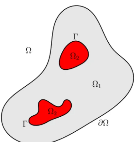
In the first part of this thesis, we study the existence and uniqueness of renormalized solution of a class of quasilinear elliptic equations posed in a two-component domain with an L1 _{data. More precisely, the domain Ω is a}

connected bounded open set in RN _{with boundary @Ω. We write Ω as the}

disjoint union Ω = Ω1 [ Ω2[ Γ, where Ω2 is an open set such that Ω2 ⇢ Ω

with a Lipschitz boundary Γ, and Ω1 = Ω \ Ω2 (see Figure 1.3). We study

the following quasilinear elliptic problem posed in Ω: 8 > > > > > > < > > > > > > : div(B(x, u1)ru1) = f in Ω1, div(B(x, u2)ru2) = f in Ω2, (B(x, u1)ru1)⌫1 = (B(x, u2)ru2)⌫1 on Γ, (B(x, u1)ru1)⌫1 = h(x)(u1 u2) on Γ, u1 = 0 on @Ω, (1.22) where ⌫1 is the unit outward normal to Ω1, f is an L1 function, and B is

a coercive matrix field which has a restricted growth assumption (B(x, r) is bounded on any compact set of R).

To properly define a renormalized solution of (1.22), we first introduce the space that we will be working with, that is well adapted to our problem.

We define the space V as

V := {v ⌘ (v1, v2) : v1 2 V1 and v2 2 H1(Ω2)},

equipped with the norm

kvk2_V := krv1k2L2_(Ω 1)+ krv2k 2 L2_(Ω 2)+ kv1 v2k 2 L2_(Γ),

Ω Ω2 Γ Ω2 Γ Ω1 ∂Ω

Figure 1.3: The two-component domain Ω where V1 is the space defined by

V1 = {v 2 H1(Ω1) : v = 0 on @Ω} with kvkV1 := krvkL2(Ω1).

We follow a similar definition from [36] with the additional term on the interface Γ and condition for the jump. More precisely:

Definition 1.7. Let u = (u1, u2) : Ω \ Γ ! R be a measurable function.

Then u is a renormalized solution of (1) if

Tk(u) 2 V, 8k > 0; (1.23a) (u1 u2)(Tk(u1) Tk(u2)) 2 L1(Γ), 8k > 0; (1.23b) lim n!1 1 n Z {|u|<n} B(x, u)ru · ru dx = 0; (1.24a) lim n!1 1 n Z Γ (u1 u2)(Tn(u1) Tn(u2)) d = 0; (1.24b)

and for any S1, S2 2 C1(R) (or equivalently for any S1, S2 2 W1,1(R)) with

compact support, u satisfies Z Ω1 S1(u1)B(x, u1)ru1· rv1dx + Z Ω1 S₁0(u1)B(x, u1)ru1· ru1v1dx + Z Ω2 S2(u2)B(x, u2)ru2· rv2dx + Z Ω2 S0 2(u2)B(x, u2)ru2· ru2v2dx + Z Γ h(x)(u1 u2)(v1S1(u1) v2S2(u2)) d = Z Ω1 f v1S1(u1) dx + Z Ω2 f v2S2(u2) dx, (1.25) for all v 2 V \ (L1_(Ω 1) ⇥ L1(Ω2)). 32

Note that since we are in the renormalized framework, a solution u of (1) may not have enough regularity to have a gradient and trace in the usual sense of Sobolev spaces. Hence, we first have to make sure that the gradient and the trace of a solution are properly defined. To this aim, we prove the following proposition (which is a generalization of [10, Lemma 2.1] and [59, Proposition 2.3]):

Proposition 1.8. Let u = (u1, u2) : Ω \ Γ ! R be a measurable function

such that Tk(u) 2 V for every k > 0.

1. For i = 1, 2, there exists a unique measurable function Gi : Ωi ! RN

such that for all k > 0,

rTk(ui) = Gi {|ui|<k} a.e. in Ωi,

where {|ui|<k} denotes the characteristic function of

{x 2 Ωi : |ui(x)| < k}.

We define Gi as the gradient of ui and write Gi = rui.

2. If sup k 1 1 kkTk(u)k 2 V < 1,

then there exists a unique measurable function wi : Γ ! R, for i = 1, 2,

such that for all k > 0,

i(Tk(ui)) = Tk(wi) a.e. in Γ,

where i : H1(Ωi) ! L2(Γ) is the trace operator. We define the

function wi as the trace of ui on Γ and set i(ui) = wi, i = 1, 2.

The originality of this definition is found in the regularity (1.23b) and the decay of the energy on the interface (1.24b), together with the presence of the term on Γ,

Z

Γ

The regularity (1.23a) and the decay of the truncated energy (1.24a) are classical and it allows us (with Proposition 1.8) to give a sense to all the integrals in (1.25) except for the boundary integral on Γ.

Indeed, let Si 2 C1(R), i = 1, 2, with compact support. Then for all

v 2 V \ (L1_(Ω

1) ⇥ L1(Ω2)), if supp Si ⇢ [ k, k] (i = 1, 2), then for i = 1, 2,

we have

Si(ui)B(x, ui)rui· rvi = Si(ui)B(x, Tk(ui))rTk(ui) · rvi 2 L1(Ωi),

S0

i(ui)B(x, ui)rui· ruivi = Si0(ui)B(x, Tk(ui))rTk(ui) · rTk(ui) vi 2 L1(Ωi),

f viSi(ui) 2 L1(Ωi).

Concerning the boundary integral on Γ, note that (1.23a) and (1.24a) are not enough to give a sense to h(x)(u1 u2)(v1S1(u1) v2S2(u2)). In general,

there is no reason to have

h(x)(u1 u2)(v1S1(u1) v2S2(u2))

= h(x)(u1 u2)(v1S1(u1) v2S2(u2)) {|u1|n} {|u2|n}

for large n.

For the boundary term, for any n 2 N, let us define ✓n : R ! R by (see

Figure 1.4) ✓n(s) = 8 > > > > > > > < > > > > > > > : 0, if s  2n, s n + 2, if 2n  s  n, 1, if n  s  n, s n + 2, if n  s  2n, 0, if s 2n.

Then since S1 has a compact support, we have for some large enough n,

h(u1 u2)v1S1(u1) = hv1(u1 u2)(S1(u1) S1(u2))✓n(u1)

+ hv1(u1 u2)S1(u2)✓n(u1).

Since ✓nalso has a compact support, then hv1(u1 u2)S1(u2)✓n(u1) is bounded,

and is therefore in L1_{(Γ). Moreover, since}

S1(u1) S1(u2) = S1(T2n(u1)) S1(T2n(u2))

and S1 are Lipschitz-continuous, we have

|hv1(u1 u2)(S1(u1) S1(u2))✓n(u1)|

 khv1kL1_(Γ)kS0

1kL1_(R)|u₁ u₂||T_2n(u₁) T_2n(u₂)|,

and we let Bε(x, t) = B(x, T1/ε(t)). We consider a solution uε 2 V of 8 > > > > > > < > > > > > > : div(Bε(x, uε1)ruε1) = fε in Ω1, div(Bε(x, uε2)ruε2) = fε in Ω2, (Bε(x, uε1)ruε1)⌫1 = (Bε(x, uε2)ruε2)⌫1 on Γ, (Bε(x, uε1)ruε1)⌫1 = h(x)(uε1 uε2) on Γ, uε 1 = 0 on @Ω.

The second step is to obtain a priori estimates, then construct (with the help of Rellich-Kondrachov compactness results) a function u such that (up to a subsequence) 8 > > > < > > > : uε i ! ui a.e. in Ω, Tk(uεi) * Tk(ui) weakly in H1(Ωi), i(uεi) ! i(ui) a.e. in Γ, i(Tk(uεi)) ! i(Tk(ui)) strongly in L2(Γ), a.e. on Γ.

The originality here comes again from the boundary integral on Γ, and using, for example, in the third step, the a priori estimate

8k > 0, (uε₁ uε₂)(Tk(uε1) Tk(uε2)) bounded in L1(Γ),

and the limit lim n!1lim sup_ε!0 1 n ✓ Z Ω\Γ B(x, Tn(uε))rTn(uε)rTn(uε) dx + Z Γ (uε 1 uε2)(Tn(uε1) Tn(uε2)) d ◆ = 0.

In the final step of the proof, we are able then to pass to the limit with an appropriate choice of test function and show that u is a renormalized solution of (1).

Remark 1.10. _{To give a sense to the integral on Γ, it is possible to replace} (1.23b) and (1.24b) by a regularity condition given by

u1 u2 2 W1

1

q,q(Γ), for some q > 1. (1.26)

This type of regularity comes from the Boccardo-Gallouët type estimates, but depends heavily on the Sobolev embedding constants. Since these constants may blow up with asymptotic analysis, we are not able to use (6). In addition, (1.26) will not work when considering a more general nonlinear problem. Thus, we chose (1.23b) and (1.24b) in the definition of renormalized solution.

To prove the uniqueness result, we adopt the method developed in [16, 38]. This method makes use of an auxiliary function ' 2 C1_{(R) with interesting}

properties. To be more precise, we use the following proposition from [38]: Proposition 1.11 ([38]). Suppose that (A4) holds. Then there exists a func-tion ' 2 C1_{(R) that satisfies the following properties:}

'(0) = 0 and '0 1.

In addition, there are constants > 1/2, 0 < k0 < 1, and L > 0 such that

'0

(1 + |'|)2δ 2 L 1_(R).

Moreover, for any r, s 2 R satisfying |'(r) '(s)|  k, for 0 < k < k0,

B(x, r) '0_(r) B(x, s) '0_(s)  1 '0_(s) Lk (1 + |'(r)| + |'(s)|)δ and 1 L  '0(s) '0_(r)  L.

One of the difficulties in the proof of uniqueness comes from the boundary integral on Γ, which is related to the jump of the solution. The following proposition is an important tool in the proof of the uniqueness theorem, which is related to the Boccardo-Gallouët estimates:

Proposition 1.12. For i = 1, 2, let i be the trace function defined on

H1_(Ω

i). Under the assumptions of Theorem 1.9, if u is a renormalized

solu-tion of (1), then i(ui) 2 L1(Γ), i = 1, 2.

The method developed in [16, 38] consists of using Tk('(u) '(v)) as test

function. The proof is very technical and is done by passing to the limit with the help of the function ✓n(u)Tk('(u) '(v)) in the renormalized formulation

in the definition of a renormalized solution.

However, the nonlinearity of the term Tk('(u) '(v)) is not compatible

with the boundary integral on Γ, since the term obtained Z

Γ

h(x)((u1 v1) (u2 v2))(Tk('(u1) '(v1) Tk('(u2) '(v2))) d

To overcome this difficulty, we show a sign property on Γ:

Lemma 1.13. Suppose assumptions (A1)–(A4) hold. If u and v are two renormalized solutions of (1), then sgn(u1 v1) = sgn(u2 v2) a.e. on Γ.

This lemma is essential in the proof of the following uniqueness theorem, which is the main result of this chapter:

Theorem 1.14. If assumptions (A1)-(A4) hold, then the renormalized so-lution of (1) is unique.

One of the major steps of the proof of Theorem 1.14 consists of showing that lim k!0 1 k2 Z Ωi ✓ 1 '0_(u i) + 1 '0_(v i) ◆ |rTk('(ui) '(vi))|2dx = 0, i = 1, 2, (1.27) where u = (u1, u2) and v = (v1, v2) are two renormalized solutions of (1),

and ' is the function in Proposition 1.11.

To prove this, after some long computations, we obtain lim sup k!0 ✓ 1 k2 Z Uk 1 ✓ 1 '0_(u 1) + 1 '0_(v 1) ◆ |r'(u1) r'(v1)|2dx + 1 k2 Z Uk 2 ✓ 1 '0_(u 2) + 1 '0_(v 2) ◆ |r'(u2) r'(v2)|2dx + 1 k2C k ◆  0, where U_ik = {x 2 Ωi : 0 < |'(ui) '(vi)| < k}, i = 1, 2, and Ck= Z Γ

h(x)[(u1 v1) (u2 v2)][Tk('(u1) '(v1)) Tk('(u2) '(v2))] d .

Hence, to show (1.27), it is enough to show that lim sup

k!0

1 k2C

k _0.

As already mentioned above, due to the presence of the function ', we don’t know in general the sign of Ck_{. The limit of} 1

k2C

k _{as k ! 0 is one}

of the main difficulties. To proceed, we use the sign property on Γ (Lemma 1.13) and we divide the set {x 2 Γ ; u1(x) v1(x) > 0} (up to a zero measure

subset) into 4 disjoint subsets,

{u1 v1 > 0} = P1[ P2[ P3[ P4,

where

P1 := {'(u1) '(v1) k} \ {'(u2) '(v2) k},

P2 := {0 < '(u1) '(v1) < k} \ {0 < '(u2) '(v2) < k},

P3 = {'(u1) '(v1) k} \ {0 < '(u2) '(v2) < k},

P4 := {0 < '(u1) '(v1) < k} \ {'(u2) '(v2) k}.

This division is possible due to Lemma 1.13. Then we are able to compute the limit of the boundary integral over each subset.

Once (1.27) is shown, we follow the same approach as in [16, 38] to show first that u1 = v1 in Ω1 (since u1 and v1 have zero trace on @Ω, which allows

us to use the Poincaré inequality). As a consequence, we have u1 = v1 on Γ.

This, combined with Lemma 1.13 and (1.27), gives u2 = v2 in Ω2.

1.2

Homogenization theory

Homogenization theory is motivated from the study of the macroscopic be-haviour of microscopic composite materials. Composite materials are com-posed of 2 or more finely mixed components and their main physical char-acteristics (e.g. thermal or electric conductivity) can be modelled by PDEs with oscillating coefficients, describing the heterogeneities at the micro-scale. Then, the mathematical homogenization theory allows to give a macroscopic description of these materials, considered as homogeneous, at the macro-scale.

There are different types of composite materials that can be studied by homogenization, some examples are plywood (a layered material) and con-crete (a periodic material). Also, additional oscillations can come, in some case, from the domain. Let us mention the ones with oscillating boundaries, such as heat radiators and engines, or perforated materials like sponge (a porous medium), or trusses.

In this thesis, we are concerned in the homogenization of finely period-ically mixed materials, that is, periodic homogenization. Indeed, when the components of these materials are finely mixed, a reasonable assumption is that the distribution of the heterogeneities is periodic.

To explain intuitively how periodic homogenization works, imagine a com-posite material with two components, Material 1 and Material 2. We suppose that an "-sized Material 1 is periodically scattered throughout Material 2, with "-periodicity in each axis-direction. This is obtained by a change of scale from a fixed unit cell (see Figure 1.2).