HAL Id: tel-01024075
https://tel.archives-ouvertes.fr/tel-01024075
Submitted on 17 Jul 2014HAL is a multi-disciplinary open access archive for the deposit and dissemination of sci-entific research documents, whether they are pub-lished or not. The documents may come from teaching and research institutions in France or abroad, or from public or private research centers.
L’archive ouverte pluridisciplinaire HAL, est destinée au dépôt et à la diffusion de documents scientifiques de niveau recherche, publiés ou non, émanant des établissements d’enseignement et de recherche français ou étrangers, des laboratoires publics ou privés.
Modelling the effects of surface roughness and a forest
litter layer on passive microwave observations:
application to soil moisture retrieval by the SMOS
mission
Heather Lawrence
To cite this version:
Heather Lawrence. Modelling the effects of surface roughness and a forest litter layer on passive microwave observations: application to soil moisture retrieval by the SMOS mission. Continental in-terfaces, environment. Université Sciences et Technologies - Bordeaux I, 2010. English. �tel-01024075�
N° d'ordre : 4207
THÈSE
PRESENTEE A
L’UNIVERSITÉ BORDEAUX I
É
COLE DOCTORALE DES SCIENCES PHYSIQUES ET DE L
’
INGENIEUR
Par Heather LAWRENCE
POUR OBTENIR LE GRADE DE
DOCTEUR
SPÉCIALITÉ : Électronique
*********************
MODÉLISATION DE L'EFFET DE LA RUGOSITÉ DE SURFACE ET
DE
LA
LITIÈRE
DES
COUVERTS
NATURELS
SUR
LES
OBSERVATIONS MICRO-ONDES PASSIVES - APPLICATION AU
SUIVI GLOBAL DE L'HUMIDITÉ DU SOL PAR LA MISSION SMOS
********************* Soutenue le : 15 décembre 2010
Après avis de :
Mme. Thuy LE TOAN Rapporteur
Mme. Jacqueline BOUTIN Rapporteur Devant la commission d’examen formée de :
M. Yann KERR Examinateur M. Francis GROUSSET Examinateur M. Jean-Pierre LAGOUARDE Examinateur M. Philippe PAILLOU Examinateur M. Jean-Pierre WIGNERON Directeur de Thèse M. François DEMONTOUX Co-Directeur de Thèse
Titre :
Modélisation de l'effet de la rugosité de surface et de la litière des couverts naturels sur les observations micro-ondes passives : application au suivi global de l'humidité du sol par la mission SMOS
Résumé :
Dans le cadre de la mission spatiale SMOS (Soil Moisture and Ocean Salinity), nous présentons dans cette thèse une nouvelle approche numérique de modélisation du calcul de l’émissivité et du coefficient bi-statique de systèmes forestiers sol-litière en Bande L. Le système sol-litière est représenté par deux couches diélectriques 3D comportant des interfaces rugueuses, une démarche qui n’apparait pas actuellement dans la littérature. Nous validons notre approche pour une seule couche en comparant les simulations de l'émissivité avec celles produites par la méthode des moments et des données expérimentales. A partir de ce nouveau modèle, nous évaluons la sensibilité de l’émissivité du système sol-litière en fonction de l’humidité et de la rugosité de la litière. Ce nouveau modèle permettra de créer une base de données synthétiques d’émissivités calculées en fonction de nombreux paramètres qui contribuera à améliorer la prise en compte de la litière dans l'algorithme d’inversion des données de la mission spatiale SMOS.
Mots clés : radiométrie micro ondes des forêts, émissivité des structures sol litière, Modélisation numérique par éléments finis, rugosité du sol, litière des forêts, HFSS, IEM, SMOSREX, Coefficient de rétro diffusion, Coefficient bi-statique, mission SMOS
Title:
Modelling the effects of surface roughness and a forest litter layer on passive microwave observations: application to soil moisture retrieval by the SMOS mission
Abstract:
In the context of the SMOS (Soil Moisture and Ocean Salinity) mission, we present a new numerical modelling approach for calculating the emissivity and bistatic scattering coefficient of the soil-litter system found in forests, at L-band. The soil-litter system is modelled as two 3-dimensional dielectric layers, each with a randomly rough surface, which to our knowledge has not previously been achieved. We investigate the validity of the approach for a single layer by comparing emissivity simulations with results of Method of Moments simulations, and experimental data. We then use the approach to evaluate the sensitivity of the soil-litter system as a function of moisture content and the roughness of the litter layer. The numerical modelling approach which has been developed will allow us in the future to create a synthetic database of the emissivity of the soil-litter system as a function of numerous parameters, which will contribute to validating and improving the inversion algorithm used by the SMOS mission to retrieve soil moisture over forests.
Key Words: microwave forest radiometry, soil-litter emissivity, FEM numerical modelling, soil roughness, forest litter, HFSS, IEM, SMOSREX, backscattering coefficient, bistatic scattering coefficient, SMOS mission
Acknowledgements
The work of this thesis was made possible by the joint financial support of the Aquitaine Region and the Centre Nationale d’Etudes Spatiales (CNES), to whom go my grateful thanks. Many people also supported me directly during my PhD, particularly in the IMS and INRA-EPHYSE laboratories in Bordeaux. I would like to thank in particular the following people:
- François DEMONTOUX for all his help and support as my PhD co-director, always willing to give me time and help when required, and to send emails and make phone calls on my behalf. I also remember especially the occasional practical joke, the wide-ranging discussions over coffee (or tea) breaks, and the banter when France were playing England, all of which provided a relaxed working environment
- Jean-Pierre WIGNERON, my PhD director, for always making time to see me when I needed help, for his constantly invaluable input and advice, and teaching, for his sense of humour and for his kindness and support during the occasional stresses of the last three years.
- The SMOS team led by Yann KERR in CESBIO laboratory, Toulouse, for making this work
possible under the SMOS umbrella. I would like to thank in particular Arnaud MIALON for his help in providing and explaining data and his collaboration on the SMOSREX 2009 soil-litter experimental campaign
- Philippe PAILLOU for the very helpful discussions around numerical modelling and radar scattering, and for his advice and input in planning the work at the early stages
My thanks go also to Liang Chen and T.D. Wu, for answering my questions by email and providing me with the AIEM model, to Marc Crapeau for kindly talking me through matlab programming one Friday afternoon, and to Alain Kruszewski for driving me the 2 hours to the SMOSREX site and back in the cold and sometimes rainy winter and for his help on the SMOSREX 2009 campaign. I would like to thank all members of INRA-EPHYSE and IMS-MCM laboratories for their support and camaraderie over the years, and would particularly like to thank the INRA “non-permanents” for the wonderful lab community they provided.
Many thanks also to my two thesis reviewers Jacqueline BOUTIN, and Thuy LE TOAN, for evaluating my work, for putting up with the short time limit we had to give and for all their helpful suggestions and corrections, and also to all members of the jury for their insightful comments and helpful discussion during the viva and afterwards.
Lastly, to all my friends and family, near or far, thank you for your love and support, in particular to: Guilherme Bontorin, Priscilla Boyer, Jérémie Brusimi, Faith Gischler, Luc Gischler, Jennifer Grant, Marie Guillot, Mena Hatchman, Stephanie Hayes, Emilie Hobday, Julien Lahoudere, Amanda Lawrence, Carol Lawrence, Hazel Lawrence, Peter Lawrence, Virginie Moreaux, Damien Parent, Tovo Rabemanantsoa, Jean-Charles Samalans, Sylvain Schnee, Alex Soudant, Katharina Spannraft, Kat Vyce, and Nathalie Yauschew-Raguenes, to name but a few of those who have greatly enriched this 3-year journey.
Contents
1. Introduction ... 2
2. Background Theory ... 6
2.1 Passive and Active Remote Sensing ... 6
2.2 Electromagnetism ... 6
2.2.1 Maxwell’s Equations ... 7
2.2.2 The Wave Equation ... 9
2.2.3 Plane Waves and Polarisation ... 10
2.2.4 A Superposition of Waves ... 11
2.2.5 The Poynting Vector... 13
2.2.6 Waves at boundaries ... 13
2.2.6.1 Reflection and Transmission coefficients for H and V polarization ... 14
2.2.6.2 Total Reflection and the Brewster Angle ... 15
2.2.6.3 Wave Propagation in a lossy medium ... 15
2.2.7 Layered media ... 18
2.2.8 Antenna Radiation ... 18
2.2.8.1 Radiation from current sources: the Hertzian Dipole ... 18
2.2.8.2 Radiation from aperture sources ... 19
2.3 Dielectric Properties of Mixtures: Effective Media ... 22
2.3.1 Physical mixing formulas ... 23
2.3.2 The Semi-empirical Refractive Mixing Formula ... 24
2.4 Radiation ... 25
2.4.2 Thermal Radiation ... 27
2.4.2.1 Black Body Radiation... 28
2.4.2.2 Non-black body Radiation and Emissivity ... 30
2.4.3 Radiative Transfer ... 32
2.4.3.1 The Radiative Transfer Equation ... 33
2.4.3.2 The Simplified Radiative Transfer Equation ... 34
2.5 Passive Microwave Remote Sensing of Land ... 35
2.5.1 Emission of Bare Soil Surfaces ... 36
2.5.1.1 The soil dielectric permittivity constant in the microwave region ... 36
2.5.1.2 Non-uniform Temperature and Dielectric profiles ... 38
2.5.1.3 Rough Surface Scattering and Emission ... 40
2.5.2 Modelling the emission of the ground covered by vegetation ... 46
2.5.3 Note ... 47
3. Modelling the Emission of the Soil-Litter system ... 50
3.1 Microwave Emission of Soil: modelling the effects of a rough surface ... 50
3.1.1 A Semi-Empirical model for soil emission at L-Band ... 52
3.1.1.1 Q-h Model Formulation ... 52
3.1.1.2 Model Development ... 53
3.1.1.3 Comparing semi-empirical models to theoretical models ... 55
3.1.2 Analytical Models ... 56
3.1.2.1 General Approach ... 56
3.1.2.2 Different Analytical Models ... 57
3.1.3 Numerical Models ... 62
3.1.3.1 Methodology ... 63
3.1.3.2 Numerical Methods ... 67
3.1.3.4 Validation of Numerical Methods ... 83
3.1.3.5 Problems of current interest ... 84
3.2 Modelling the contribution of the litter layer to forest emission at L-band ... 85
3.2.1 The Forest structure ... 85
3.2.2 Remote Sensing of Forests ... 88
3.2.2.1 Experimental data ... 88
3.2.2.2 Theoretical Models ... 88
3.2.3 Discussion ... 94
3.3 Choice of approach for modelling the soil-litter L-band emission in this thesis ... 96
4. The Numerical FEM Approach developed for Calculating the L-band Scattering and Emission of the Soil-Litter system found in Forests ... 102
4.1 Model Description ... 102
4.1.1 Ansoft’s HFSS software ... 102
4.1.2 Calculating the scattering and emission of forest multilayer structures using a numerical FEM approach ... 103
4.1.2.1 Building the structure ... 105
4.1.2.2 HFSS Simulations ... 107
4.1.2.3 Analysing Results calculated by HFSS ... 111
4.1.3 Note ... 112
4.2 A sensitivity analysis to set model parameters ... 112
4.2.1 Model Parameters and calculation conditions ... 113
4.2.2 Method and Results ... 116
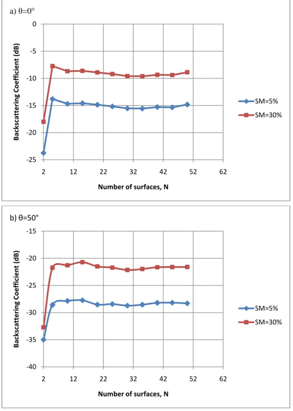
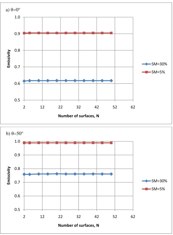
4.2.2.1 Number of Rough Surfaces ... 116
4.2.2.2 Integration step, s... 128
4.2.2.4 Surface size ... 139
4.2.2.5 Calculation Cost ... 142
4.2.3 Conclusions: Values determined for model parameters ... 143
5. Validation of the Numerical FEM Approach for a Single Layer ... 146
5.1 Comparison with Fresnel for a flat surface ... 146
5.1.1 HFSS calculation set up... 146
5.1.2 Results and Conclusions ... 147
5.2 Comparison with the Method of Moments for a rough surface... 149
5.2.1 Method of Moments data ... 149
5.2.2 Method ... 150
5.2.3 Results ... 151
5.2.4 Conclusion ... 155
5.3 Comparison between the numerical approach, experimental data and the AIEM model .... 156
5.3.1 SMOSREX 2006 dataset ... 156
5.3.2 Method ... 162
5.3.3 Results and Discussion ... 163
5.3.4 Conclusions ... 170
6. Emissivity of the Soil-Litter system: comparison with Experimental Data and the Schwank Model ... 172
6.1 The Bray 2009 Experimental campaign and the Schwank model predictions ... 172
6.3 Results and Discussion ... 178
6.4 Conclusions and Perspectives ... 182
7. Conclusions ... 186
8. Perspectives ... 190
9. Appendix A : Résumé en Français ... 194
List of Symbols and Abbreviations
α: attenuation constant, a measure of the attenuation of an electromagnetic wave as it travels through a lossy medium
AIEM: Advanced Integral Equation Method
β': phase constant, a measure of the change of phase experienced by an electromagnetic wave when it enters a lossy medium
B: Magnetic Field
c: speed of an electromagnetic wave
c0: speed of an electromagnetic wave in a vacuum, equal to 3x10 8
ms-1 D: Electric displacement field
ep: emissivity at polarisation p
eN: emissivity calculated by averaging the scattered electric field over N surfaces
ε: electric permittivity of a material
ε0: electric permittivity of a vacuum, equal to 8.85x10⁻¹² F/m
εr: the relative permittivity (electric permittivity relative to that of a vacuum)
E: Electric Field
f: frequency of an electromagnetic wave Ff: spectral flux density at frequency f
F: radiative flux density FEM: Finite Element Method
FDTD: Finite Difference Time Domain Method
γ: propagation constant, a measure of the change in phase and magnitude of a wave as it enters a lossy medium
h: Planck’s constant, equal to 6.26x10⁻³⁴ Js-1 H: magnetising field
HFSS: High Frequency Software Simulator, electromagnetic modelling software used in this PhD I: electric current
If: specific intensity, or brightness, of a radiated beam
IEM: Integral Equation Method
J: surface current density (current per unit area) k: the wave number of an electromagnetic wave kb: Boltzmann constant, equal to 1.381x10
-23
JK-1 KA: Kirchoff Approximation
λ: wavelength of an electromagnetic wave
λ0: wavelength of an electromagnetic wave in a vacuum
L: size of the rough surface, also equal to the width of the calculation area Lc: autocorrelation length of a rough surface
L-MEB: L-Band Microwave Emission of the Biosphere model m: rough surface slope, equal to σ/Lc
mg: gravimetric soil moisture content
mv: volumetric soil moisture content
µ: magnetic permeability of a material
µ: the direction of propagation cosθ
µ0: magnetic permeability of a vacuum, equal to 4πx10-7 H/m
µr: the relative permeability (magnetic permeability relative to that of a vacuum)
MoM: Method of Moments n: refractive index of a wave
N: number of simulations performed for a given roughness condition p: penetration depth of a medium
P: power
ρ: the volume charge density
ρ(x’,y’): autocorrelation function of a rough surface
ρxy: degree of coherence of a wave, where the symbols x and y refer to the wave’s components
ρb: soil bulk density
ρw: density of water
Rp: Reflection coefficient for a wave of polarisation p
RTE: Radiative Transfer Equation
σ: the standard deviation of surface heights of a rough surface, also used for a material’s conductivity
σΝ: the bistatic scattering coefficient calculated by averaging the electric field over N surfaces
σsb: Stephan-Boltzmann constant
σpq 0
: bistatic scattering coefficient at polarisation p of the incident beam and polarisation q of the scattered beam
σ0
: backscattering coefficient
s: the step in angles (θS,φS) at which the scattered field is calculated, equivalent to the integration step
for the emissivity calculation S: Poynting vector
SMOS: Soil Moisture and Ocean Salinity mission
SMOSREX: Surface Monitoring Of the Soil Reservoir EXperiment
θ: angle of incidence for scattering problems, equivalent to the angle of emission
θT: angle of transmission when a wave encounters a boundary
θB: Brewster angle: the incident angle at which total transmission occurs for a V polarised wave
(θS, φS): scattering angle
τ: optical depth of a medium
Tp: Transmission coefficient for a wave of polarization p
Γ: reflectivity
Τ: transmissivity T: temperature
Teff: effective temperature of a medium
TB(θ,φ): Brightness temperature at angle (θ,φ)
uf: spectral energy density (at frequency f)
u(T): energy density of a radiated beam
ω: angular frequency of an electromagnetic wave, also used for a medium’s single scattering albedo W(z): temperature weighting function for each layer in the soil
1
2
1.
Introduction
Remote sensing is the collection of information about objects from a distance. As a discipline it first became possible with the advent of balloons (1900), and later airplanes, providing a platform for regarding the environment. In 1960 the first satellite weather image was taken with NASA’s TIROS mission, heralding the start of remote sensing as a tool for observing the environment.
Remote Sensing of the environment via satellite or airplane allows us to obtain geophysical information over large regions. The satellite or airplane provides a platform at a distance, from which a signal from the environment can be measured, usually an electromagnetic wave. This signal must be propagated between the object and the observer unambiguously and without serious loss. Ideally propagation should be in a straight line with no attenuation (from vegetation cover, or the atmosphere for example), in other words through a transparent, homogeneous medium. An interaction must also exist between the sensing wave and the object, in order to provide the observer with information about the object.
Remote Sensing of the environment combines many disciplines, principally electromagnetic theory and environmental studies. In order to obtain useful information from remote sensing observations we must understand the electromagnetic theory describing the processes involved in the propagation and interactions of electromagnetic waves as well as how the observed objects interact with these waves. This must be coupled with an understanding of key environmental and geophysical properties and how they affect such interactions. Often this means understanding the electromagnetic properties of the object and how they depend on its physical properties. For example a key electromagnetic property is the dielectric permittivity constant which can be linked to properties such as moisture content, material content, temperature, etc. Also an object’s shape can affect its interaction with electromagnetic waves. Environmental variables that can be measured by remote sensing include physical variables such as vegetation and ground structure and global variables such as the Earth’s water content, salinity, and temperature.
The work of this PhD thesis was carried out in the context of the European Space Agency’s (ESA’s) Soil Moisture and Ocean Salinity (SMOS) mission (Y. Kerr et al 2001), a remote sensing satellite mission. The SMOS mission was launched in November 2009 with the objective of retrieving the soil moisture over land and the salinity over oceans on a global scale, from microwave radiometric measurements of the Earth’s thermal radiation. The Earth’s thermal emission is very sensitive to these two variables in the L-band microwave region and the mission was conceived in order to provide a way to measure globally these two variables, which had not previously been done.
3
Surface soil moisture is a key variable in the hydrologic cycle. Both water and energy fluxes at the surface/atmosphere interface depend strongly on soil moisture and surface soil moisture drives evaporation, infiltration and runoff while soil moisture in the vadose zone (the top part of the soil which is unsaturated by water) governs the rate of water uptake by the vegetation. Global soil moisture is an important input variable for numerical weather forecasting and climate models, such as the European Centre for Medium-range Weather Forecasts’ (ECMWF’s) Numerical Weather Prediction (NWP) model.
The SMOS satellite carries an interferometric radiometer which measures the Earth’s natural thermal emission, at L-band. This band was chosen because at higher frequencies the vegetation cover is not transparent enough to allow us to measure the soil signal and at lower frequencies we are not able to obtain a very good resolution of the image taken by the satellite. The frequency at which the SMOS satellite radiometer takes measurements is 1.4 GHz, since this is the L-band frequency designated by the International Telecommunication Union for passive remote sensing measurements. Note that volume effects cannot be entirely neglected at this frequency: in general the Earth’s emission includes mainly contributions from the surface (on average the first 3-5cm) at this frequency but for low soil moisture conditions the emission also includes contributions from much lower depths.
These measurements are taken at a mixture of the two polarisations H and V, from which the pure H and V components can be calculated and at angles in the range of 0° to 50°. A retrieval algorithm is then applied to the measurements in order to retrieve soil moisture. This algorithm models emission using the forward model and then uses an iterative approach, obtaining values of soil moisture and surface parameters which minimise a cost function computed from the sum if the square weighted differences between measured and modelled emission. The forward model is the so-called L-band Microwave Emission of the Biosphere (LMEB) model (Wigneron et al 2003, 2007). This model is the result of an extensive review of current knowledge of microwave emission of various land cover types with the objective of being accurate while remaining simple enough for operational use at a global scale, and allowing developments to be incorporated as they occur.
Other factors affecting microwave emission include surface roughness, topography, soil texture, land cover and vegetation type. All these factors are constant with time and so can be estimated or calibrated from other information such as soil maps, data taken in the optical domain, digital elevation maps, etc. Only vegetation cover is retrieved simultaneously to soil moisture, making use of multi-angular, dual-polarisation measurements.
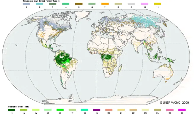
For the work of this thesis we concentrate on soil moisture retrieval over forests. The ground emission in forests is affected by the vegetation above the ground which consists of a tree, or canopy, layer and a litter layer of organic debris covering the forest floor. The canopy acts as a semi-transparent layer which attenuates the ground emission and this can be modelled simply by the τ-ω model, with two
4
variables, the optical depth τ and the scattering albedo ω, determining the attenuation. However the litter layer is much denser and has a tendency to absorb and hold water which means that, besides attenuating the ground emission, it adds an emission of its own to the signal which is very strong under high moisture conditions. In addition both the ground and the litter layer often have rough surfaces, which affect the overall emission. The litter layer effectively masks the ground signal (Grant 2007, 2009) making it difficult to retrieve soil moisture. This effect has not been studied in any great depth and has not been well accounted for in the L-MEB model and so although soil moisture retrieval is performed over forests in the SMOS mission its accuracy has yet to be determined and is expected to be poor.
The motivation of this PhD thesis is to improve the L-MEB model over forests by studying in greater depth the contribution of emission from the forest floor, including the soil and litter layers, to the signal. In order to do this we aim to develop a modelling approach which allows us to calculate the emission of the soil and litter layers in forests, incorporating surface roughness of both the soil and litter layers as well as parameters relating to both layers. The advantage of a modelling approach over an experimental one is that we can better control many different parameters that effect the emission. Once developed and validated, the model can be used to create a large database of the emission of the soil-litter system, as a function of numerous parameters. Analysing results in this database, we hope to infer a simple model which can be incorporated into the L-MEB forward model to better account for the effect of a litter layer in forest emission.
The work of this PhD was to develop and validate the model to be used for modelling the soil-litter layers. Such a model requires at least two layers and surface roughness and there is currently no numerical (exact) model available for this. Although generating the database is not part of this thesis, the model must be developed with this end goal in mind.
In the following chapters we present first the background theory including the physics relevant to remote sensing of the environment and the theory for the microwave emission of forests. Secondly we present a review of the methods currently used to model the bare soil layer, and secondly methods for modelling the litter layer. The main challenge in modelling the soil layer is in modelling the surface roughness and so we concentrate mainly on this in the soil layer section. Next we present the model developed in the work of this thesis and validate it against other models and experimental data. We finish with a conclusions and perspectives section.
5
6
2.
Background Theory
In this section we present the background theory relevant to this thesis. The information presented is mainly based on the volumes by Ulaby et al (1985a,b and c) but also on the remote sensing lecture course by C. Matzler (2007), and the volumes by C. Matzler et al (2006) and Chukhlantsev (2006). We begin with the context of active and passive remote sensing of the environment, two distinct areas of research that are nevertheless theoretically linked. We then present a summary of the physical theories of electromagnetism and thermal radiation, on which active and passive remote sensing respectively are based. We then present the background theory for passive microwave remote sensing of land. In this section we focus in particular on modelling the bare ground emission as well as the emission of the ground covered by vegetation, topics which are key to this thesis.
2.1
Passive and Active Remote Sensing
Methods for observing the environment by remote sensing can be divided in two distinct categories: active and passive. In active methods an artificially created electromagnetic wave is sent to the object to be sensed and the returned signal analysed. In passive methods it is the environment’s natural thermal emission that is detected and analysed. Thus for the active case we focus on scattering from the material and in the passive case we focus on emission. The theory behind active remote sensing is based on the theory of electromagnetism whereas the theory behind passive remote sensing is based on radiation theory. In the following sections we present these two theories, focusing on areas that are important for remote sensing. As we will see electromagnetic theory relating to scattering can be linked to the concept of emission found in thermal radiation, by Peake’s theorem (1959): we can calculate an object’s emission by integrating the scattering resulting from an incident wave. Thus, although experimentally passive and active remote sensing techniques each provide different information about an object, theoretically we can calculate one from the other. In this thesis we are interested in the emission of soil-litter systems. However in theoretical modelling approaches it is usual to calculate the emission from the scattering, including the approach we develop and apply. We will therefore present the theory behind both electromagnetic scattering and thermal radiation as both are relevant to this thesis.
2.2
Electromagnetism
The theory of electromagnetism was formulated by Maxwell. It describes the behaviour of magnetic and electric fields for a given system of electric currents and charges. It is a macroscopic theory and so does not consider the microscopic processes in a medium in the presence of an electromagnetic field. Electric and magnetic properties of a specific medium are described by three macroscopic quantities: the magnetic permeability, , the conductivity σ and the permittivity ε. Electromagnetic theory rests on
7
Maxwell’s four equations. These four equations are very powerful since they are simple, yet fully describe an electromagnetic field problem: all electromagnetic theory can be derived from them.
2.2.1
Maxwell’s Equations
Maxwell’s four equations can be expressed in differential or integral form. In differential form they can be written as:
ρ = ∇.D (2.1a) 0 B . = ∇ (2.1b) t B E x ∂ ∂ − = ∇ (2.1c) J t D H x + ∂ ∂ = ∇ (2.1d) where: E D=ε (2.2) H B=µ (2.3) E J=σ (Ohm’s law) (2.4)
and the electromagnetic quantities are: E: the electric field
B: the magnetic field
D: the electric displacement field H: the magnetising field
ε: the electric permittivity
ρ: the volume charge density
σ: the conductivity
8
ε and can be expressed as functions of the vacuum permittivity ε0 and the vacuum permeability 0 as
follows:
(2.5) (2.6) where εr and r are respectively the relative electric permittivity and magnetic permeability of the
material. Both ε and and equivalently εr and r are usually complex and are often written as:
" " (2.7)
" " (2.8)
Note that in this thesis we deal with non-magnetic media, i.e. r = 1.
Maxwell’s equations can be written in their integral form as:
0 A d . E V =
∫∫
∂ (2.9a) 0 A d . B V =∫∫
∂ (2.9b) t l d E B,S S ∂ Φ ∂ − = ⋅∫
∂ (2.9c) t I l d B 0 S 0 0 E,S S ∂ Φ ∂ ε µ + µ = ⋅∫
∂ (2.9d) The left-hand sides of (2.9a) and (2.9b) are the integration of respectively the electric field and magnetic field over a closed surface ∂V, of area A and bounding volume V. The left-hand sides of (2.9c) and (2.9d) are the integration of respectively the electric field and magnetic fields over closed line dS of length l bounding area S.ФB,S is the magnetic flux through area S and ФE,S is the electricflux through area S, given by:
∫∫
⋅ = Φ S S , B B dA (2.10a)∫∫
⋅ = Φ S S , E E dA (2.10b)For the work of this thesis, we develop a numerical modelling approach to calculate the emission of the forest soil-litter system. Numerical modelling approaches such as the one used in this thesis solve Maxwell’s equations for finite spaces. This is what makes them exact, since Maxwell’s equations are exact and complete. As will be covered in more detail in section 3.1.3, numerical modelling
9
techniques can be divided into two types: those that solve Maxwell’s equations in their differential form and those that solve them in their integral form.
2.2.2
The Wave Equation
For active remote sensing we are interested in the scattering of electromagnetic waves. We now consider, therefore, the concept of electromagnetic waves, which may be derived from Maxwell’s equations. Maxwell’s theory permits the existence of electromagnetic fields in space even without the presence of charge or current sources. This is because a changing magnetic field creates a changing electric field and vice versa. We can therefore visualise an electromagnetic wave propagating through space with oscillating electric and magnetic fields which are dependent on each other. In order to formally describe such waves we combine Maxwell’s equations (grad x (2.1c)) to obtain two wave equations, which, for a non-conductor (σ=0), are given by:
0 t E c E 2 2 2 0 r r 2 = ∂ ∂ ε µ − ∇ (2.11a) 0 t B c B 2 2 2 0 r r 2 = ∂ ∂ ε µ − ∇ (2.11b) For: 2 1 0 0 0 ( ) c = ε µ (2.12)
Electromagnetic waves propagate with phase velocity c given by:
r r 0/ c c= ε µ (2.13)
where c0 is the speed of an electromagnetic wave in a vacuum equal to 3x10 8
ms-1.
It further follows from Maxwell’s equations that a wave’s electric and magnetic fields must always be perpendicular; hence if the electric field oscillates in the x direction, the magnetic field oscillates in the y or z direction. The magnitudes of the E and B fields are also related by:
c / E
B0 = O . (2.14)
For this reason we usually only consider the electric or magnetic fields in waves since the other can be derived afterwards.
10
2.2.3
Plane Waves and Polarisation
There are numerous possible solutions to the wave equation and correspondingly numerous types of wave, of which the most basic form is the plane wave. In remote sensing we deal extensively with plane waves since antennas emit waves that may be considered plane far from the emitting antenna and also the earth’s thermal radiation may be considered plane when measured at a distance far from the ground.
A plane wave propagating in an arbitrary direction given by the wavevector k can be described by the following equations: ) t . r ik exp( E ) t , r ( E = 0 ⋅ −ω (2.15a) ) t . r ik exp( H ) t , r ( H = 0 ⋅ −ω (2.15b)
where ω is the phase velocity. Note we take the real part in the above equations but it is common practice to write wave equations in complex form and the real part is implied. A wave is considered to be plane when its electric field remains in the same plane with respect to its propagation.
Substituting these wave equations into Maxwell’s equations (2.1a) and (2.1b) we find that k is perpendicular to both H and E as follows: ∇⋅H=ik⋅H=0and ∇⋅E=ik⋅E=0.
Since the electric and magnetic fields must also be perpendicular these two fields form a plane orthogonal to the direction of propagation, called the polarisation plane.
Inserting the above equations into the wave equation we deduce the following relationship:
c 1 1 k = εµ = ω (2.16)
ω is calculated as 2π/λ, where λ is the wavelength. This equation for k is the dispersion relation of
electromagnetic waves in unbounded space.
A wave is linearly polarised if its electric and magnetic fields oscillate in one direction only. However all waves can be rewritten as the sum of their components in the 2 orthogonal polarisations. In particular, a wave incident on a plane boundary at angle θi has an electric field which can be
decomposed into two directions: the direction orthogonal to the boundary plane and the direction parallel to this plane:
//
E E
11
The orthogonal component is also known as the vertical component (V) and the parallel component is also known as the horizontal component (H). Horizontal and Vertical polarisations are not intrinsic to a plane wave but rather depend on the wave’s orientation relative to a boundary. A horizontally polarised wave has an electric field only in the H direction and a vertically polarised wave has an electric field in the V direction only, relative to the boundary.
Figure 2.1: One period of a plane EM wave with linear polarization (direction of the E field is constant). The horizontal axis is the phase kr-ωt with the propagation path, r.
In remote sensing we usually consider waves that are either H or V polarised: in active remote sensing we direct these polarised beams at the environment and also measure the reflections and passive emissions at both H and V polarisation (for example the SMOS satellite measures emission at a mixture of H and V polarisation and the H and V components are then calculated from this measurement). This provides us with two sets of measurements instead of one, and allows us to better retrieve environmental parameters.
2.2.4
A Superposition of Waves
Previously we have considered plane waves of a single frequency, known as monochromatic waves. Signals transmitted from single frequency or multifrequency transmitters are of this type. A wave that is not monochromatic but essentially behaves like one is said to be quasi-monochromatic.
Electromagnetic signals emitted by physical objects, irregular terrains or inhomogeneous media usually cover a wide range of frequencies and consist of a superposition of many statistically independent waves. There is no correlation between the component waves of this type of signal which is said to be incoherent or unpolarised.
12
To identify the state of polarisation or degree of coherence of a wave, Born and Wolf (1964) and others (Ko 1962, Kraus and Carver 1973) introduced the following relationship:
2 1 2 y 2 x y x xy E E * E E = ρ (2.18)
ρxy is equal to 1 when the wave is completely polarised and 0 when the wave is completely
unpolarised. ρxy between these two values is said to be partially polarised or partially coherent.
The concept of coherence more generally describes all properties of the correlation between physical quantities of a wave. When considering the addition of two waves with electric field vectors E1 and E2
we calculate their coherence from:
2 1 2 2 2 1 2 1 12 E E * E E = ρ (2.19)
Often the concept of coherence refers to the amplitudes of two waves relative to each other: two waves are said to be coherent if they have a constant phase relative to each other. Note that if two waves add incoherently the power of the resultant wave is the algebraic sum of the powers of its components. For example, let us consider two beams E1 and E2 which are combined to form a beam E1+E2. The power
of this combined beam is then proportional to:
* 2 1 2 2 2 1 2 2 1 E E E 2 E E E + = + + (2.20)
If the beams are incoherent the third term on the right-hand side of (2.20) is equal to zero thus the amplitude of the resultant wave is the algebraic sum of the amplitudes of its components. However if the waves are coherent this term is not zero and we have what is called coherent effects. This means we see peaks and troughs in the amplitude of the combined beam, depending on whether the two components add in phase or out of phase. In radiometry because the emission is natural it is on the whole incoherent. However, in scattering coherent effects are more often seen since the beam measured is artificially created and therefore monochromatic and also multiple reflections occur which lead to coherence effects.
The concept of a coherent and an incoherent beam is important when considering rough surface scattering, as will be described in section 2.5.1.3.
13
2.2.5
The Poynting Vector
We now consider the energy carried by an electromagnetic wave, which can be calculated from the Poynting vector. The complex Poynting vector, S, is defined as:
H E
S= × (2.21)
The Poynting vector is perpendicular to the electric and magnetic fields and so is in the direction of propagation. It represents the energy flux, or the power per unit area of the wave. A wave’s energy is therefore always transferred in the direction of propagation and the amount of energy transferred by a wave per unit area and per unit time is given by ½ times the real part of S. Since the magnitude of the electric and magnetic fields are related by (2.14) the energy of a plane wave is thus proportional to the square of the electric field, or the square of the magnetic field.
It is important to note this because in the field of scattering, we often measure how much energy is scattered in different directions.
2.2.6
Waves at boundaries
So far we have considered the basics of electromagnetic theory (Maxwell’s equations) and the properties of electromagnetic waves. We turn now to the scattering of electromagnetic waves at a boundary, which is important for the work of this thesis, since our numerical approach calculates the scattering of an electromagnetic wave off the boundary of the soil-litter system.
When a wave approaches a boundary, that is to say a change in the electromagnetic properties of the medium through which it propagates, there are certain rules governing its behaviour. The electric field, E, perpendicular to the boundary must be the same either side of the boundary and the magnetic field, H, parallel to the boundary must be conserved. This leads to some of the wave being transmitted, at angle to the normal, θT, and some of the wave being reflected, at angle θ to the normal, see Figure 2.2
θT θ θ Medium 1 ε1, 1 Medium 2 ε2, 2
Figure 2.2: Reflection and transmission of an electromagnetic wave at a plane boundary
14
for example. In sections 2.2.6.1 - 2.2.6.3 we consider the amplitudes and behaviour of the transmitted and reflected beams.
2.2.6.1
Reflection and Transmission coefficients for H and V polarization
The fraction of the wave that is reflected and the fraction transmitted can be calculated by the following Fresnel formulas, which are derived directly from the boundary conditions:
T 1 2 T 1 2 h cos Z cos Z cos Z cos Z R θ + θ θ − θ = (2.22) θ + θ θ − θ = cos Z cos Z cos Z cos Z R 1 T 2 1 T 2 v (2.23) (2.24) (2.25)
where Z, the material impedance, is the electric field divided by the magnetic field, equal to:
k i H E Z eq ω µ − = ε µ = = (2.26)
The reflectivity, Γ, and transmissivity, T, are the square of respectively the reflection coefficient and the transmission coefficient. The reflectivity is the fraction of the incident power that is reflected and the transmissivity is the fraction of incident power that is transmitted. From energy conservation we have: 1 = Τ + Γ (2.27)
The reflection and transmission coefficients are the fractions of the incident wave amplitude reflected and transmitted respectively.
The angle of transmission θT can be calculated from the incident angle θas follows:
2 1 T k sin k sinθ = θ (2.28) T 1 2 2 h cos Z cos Z cos Z 2 T θ + θ θ = θ + θ θ = cos Z cos Z cos Z 2 T 1 T 2 2 v
15
where k1 is the wavenumber in medium 1 and k2 the wavenumber in medium 2. This relationship is
known as Snell’s law since it was originally found by Snell, and can also be derived from the boundary conditions.
2.2.6.2
Total Reflection and the Brewster Angle
Two phenomena of interest relating to plane wave reflection and transmission across a plane boundary between lossless media are total reflection and total transmission. These two can be derived from Snell’s law.
Total reflection occurs when a wave is incident from a more optically dense to a less optically dense medium (k1>k2) and the incident angle is greater than the critical angle θc, such that:
1 2 c k k sinθ = . (2.29)
Inserting this value into Snell’s law we find that cosθ2 is entirely imaginary for θ1≥θc and thus the
wave is completely reflected; no average energy can be transmitted into the lower medium. This phenomenon is true for both H and V polarised waves.
Total transmission occurs for V polarised waves at an incident angle equal to the Brewster angle, θB,
where: 2 1 1 2 B tan ε ε = θ (2.30) This follows directly from Snell’s law if we let R=0.
This effect can be understood qualitatively by considering electric dipoles in the medium. The incident field is absorbed by the medium and then reradiated by oscillating electric dipoles at the interface. The dipoles oscillate in the polarisation direction of the transmitted wave, the same oscillation producing the reflected beam. However dipoles cannot radiate any energy along their direction of oscillation. Therefore when the direction of the refracted beam is perpendicular to the direction of the reflected beam, as is the case at the Brewster angle, the dipoles cannot radiate any energy in the reflected direction and total transmission occurs.
2.2.6.3
Wave Propagation in a lossy medium
If medium 2 in figure 2.2 has a relative permittivity constant with a non-zero imaginary part, then the transmitted wave experiences a loss in energy as it travels through this medium, associated with the
16
imaginary part of the permittivity. To illustrate this, let us consider a wave propagating in the z direction through an isotropic medium with complex relative permittivity εr and complex relative
permeability µr. Inserting (2.16) into (2.15a) (and setting µr=1) we find that the electric field can be
expressed as: z x x E e E = −γ (2.31a) z y y E e E = −γ (2.31b) z z z E e E = −γ (2.31c)
The electric and magnetic fields are both perpendicular to each other and to the direction of travel of the wave. Let us therefore take the E field to be entirely in the y direction and the H field in the x direction.
γ is the propagation constant and is complex since it depends on εr and r, which are both complex. It
can be written as:
' β α γ = +i
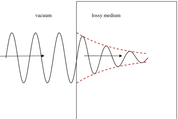
(2.32) where α is the attenuation constant and β’ is the phase constant. Thus a wave travelling in a lossy medium, i.e. one with non-zero values of εr”and/or µr”, will be attenuated by a factor of e
-α
. Figure 2.3 shows a representation of this. A wave passing from a vacuum to a medium will also undergo a phase change of +β’.
17
From Maxwell’s equations we find that α and β’ depend on the medium permittivity and permeability as follows: + + δ ″ ε ″ µ − ′ ε ′ µ β = β′ 2 tan 1 1 2 r r r r 0 (2.33) p 1 2 tan 1 1 2 r r r r 0 = − + + δ ″ ε ″ µ − ′ ε ′ µ β = α (2.34)
Where β0 and tanδ are given by:
0 0 2
λ
π
β
= (2.35) ″ ε ″ µ − ′ ε µ ″ ε µ + ′ ε ″ µ = δ r r r r r r r r tan (2.36)p is the penetration depth, the distance the wave must travel through the medium to be attenuated by a factor of 1/e. The penetration depth is an important idea for emission in electromagnetism, since it turns out that the ground emits thermal emission from a depth related to the penetration depth (see section 2.5.1.2)
vacuum lossy medium
Figure 2.3: the amplitude of a wave passing from a vacuum to a lossy medium. The wave’s magnitude is attenuated exponentially in the lossy medium. Note that the phase change is not shown
18
2.2.7
Layered media
Plane boundary reflection and transmission can be generalised to a multilayer case. This is done by evaluating the fields within each layer and then applying a matrix technique to sum the effects of all layers. The current models which include the litter layer in forest scattering and emission use this type of technique since the soil and forest litter make up a two layer system. However this technique only applies to plane boundaries, where the surfaces are flat.
2.2.8
Antenna Radiation
In the previous sections we considered the properties and behaviour of electromagnetic waves. Now we will consider how these waves may be created, by antennas. This is not directly relevant to the work of this thesis which involves numerical modelling in which we consider the scattering of a wave, but not its creation, but the theory of antenna radiation leads to the important concepts such as the near and far field, which will be important later for numerical modelling.
The radiation of an antenna, or the launching of a free space wave, may be viewed in two different ways: as radiation from current sources or as radiation from apertures. These lead to different approaches for calculating the radiated electromagnetic field. The theory for antenna radiation is also relevant to emitting objects since they can be modelled as antenna.
2.2.8.1
Radiation from current sources: the Hertzian Dipole
The short dipole or Hertzian dipole has a length l which is much less than the wavelength. The fields E and H at a distance Q are induced by the current Iacross the dipole, which we can assume to be uniform. A linear antenna may be regarded as a series of a large number of short antennas and the field due to the linear antenna can then be calculated by integrating the fields induced by all elements, including magnitude and phase.
We assume the current in the short dipole to be sinusoidal:
t i oe
I
I= −ω (2.37)
The fields E and H induced by the antenna can be calculated from the vector potential A, to be:
θ + π η = cos kr i 2 r 2 e 4 l I E 3 2 ikr 0 r (2.38a) θ + + − π η = θ sin kr i r 1 r ik e 4 l I E 3 2 ikr 0 (2.38b)
19 θ + − π = φ sin r 1 r ik e 4 l I H 2 ikr 0 (2.38c)
where , and Er and Eθ are the components of the electric field in the r and θ direction
respectively, in spherical polar coordinates, and Hφ is the component of the H field in the φ direction. It is important to note that at large distances, kr>>1, the 1/r term is much larger than the 1/r2 and 1/r3 terms in the above equations. Thus the fields reduce to:
ikr 0 e sin r 4 l ikI E θ π η − = θ (2.39a) η = θ π − = θ φ e sin E r 4 l ikI H 0 ikr (2.39b)
and Er is negligible. This is known as the “far field region” and we see that in this region the fields
produced by the Hertzian dipole are similar to uniform plane waves
2.2.8.2
Radiation from aperture sources
In this case the radiated field is related to the field distribution across the aperture, which becomes the radiation source. There are two types of formulation: the scalar formulation based on Kirchoff’s work and the vector formulation based on Maxwell’s equations. The latter is theoretically superior but more difficult and so is used mostly for apertures whose dimensions are less than or comparable to the wavelength, making the scalar approach inapplicable. In this section we will only consider the simpler scalar approach.
a) Scalar Approach
Let us consider an aperture in the plane (xa,ya) of length d and either an observation plane (x,y) at a
fixed distance z from the aperture or an observation sphere at fixed radius r=R from the centre of the aperture, as shown in Figure 2.4:
20 observation sphere at fixed radius R R R n
Figure 2.4: Far-zone observation regions: (a) plane at a fixed distance, and (b) sphere at a fixed radius r=R
Starting with Green’s theorem and the Helmholtz wave equation and applying the Kirchoff boundary conditions we can derive a formula relating the field at a distance (x,y,z) from the aperture to the field distribution across the aperture Ea(xa,ya):
∫∫
θ − θ − π = aperture a a 2 1 iks a a a ik cos ikcos dx dy s 1 s e ) y , x ( E 4 1 ) z , y , x ( E (2.40)where θ1 is the angle between the normal to the aperture, , and the observation point and is the angle between and the direction of the incident wave illuminating the aperture. s is the vector defining the direction of propagation of the wave.
d xa aperture plane θ1 d xa aperture plane x observation plane at fixed distance z z r θ1
21
This integral is known as the Fresnel-Kirchoff diffraction integral. We can use approximations to simplify the computation of the integral, namely the Fresnel and Fraunhofer approximations. These approximations explain the important concepts of the near field and far field zone and the intermediate Fresnel zone.
a1) Near Field zone
The immediate vicinity of the aperture is called the near-field region. In this region no approximations may be applied to solve the Fresnel-Kirchoff diffraction integral. Furthermore the integral itself may not be valid in this region because the Kirchoff boundary conditions applied in its derivation are not valid and so vector diffraction theory should be used.
a2) Fresnel Region
In the Fresnel region, intermediate between the near field and far field, the assumption is made that the distance z from the aperture to the observation plane is much larger than the longest linear dimension of the aperture (i.e. aperture length l). Since the aperture is much smaller than the wavelength for the scalar approach to be applicable the distance z is much larger than the wavelength. The following approximations can therefore be applied:
ik ik s 1 ≈− − (2.41a) θ ≈ θ cos cos 1 (2.41b) r e s eiks ≈ iks (2.41c)
We also replace s=
[
z2+(x−xa)2+(y−ya)2]
1/2 by the first two terms of its binomial expansion;1 ! ! " (2.42)
This latter approximation is called the Fresnel approximation.
Substituting these approximations into the Fresnel-Kirchoff diffraction integral we obtain:
# $, &, ' ()*+,- ./012$3 4'5 $ & 6 7 8 $, &, (2.43) where 8 $, &, 9 #;; : $:, &: 2$3 4'5 $ & 6 2$34 '5 $$: &&: 6 <$:<&: (2.44)
22
a3) Fraunhofer, far-field, region
If the observation point is far enough away such that:
= > 5 $: &: ?: (2.45)
then exp 4 CDE xF yF HFI6 1 over the aperture and we have:
# $, &, '.-L/0K8 , M (2.46)
where:
8 , M N #;; : $:, &: 2$3OP Q $:RS M &: M T<$:<&: (2.47) In practice these equations are used for the Fraunhofer conditions:
= > U-V (2.48)
which is known as the far-field condition, and is obtained by requiring:
5
L $: &: ?: W X
Y (2.49)
and choosing the origin to be the midpoint of the longest dimension of the aperture.
So we see that when objects emit electromagnetic radiation the emitted fields have a different form near and far from the receiver. When radiation is measured by a satellite borne detector it is the far field that is measured. This is important for our numerical model since Maxwell’s equations are solved in the near field but we require the far field value. In this case a near to far field transformation is applied to the solution, by treating the external surfaces as aperture antennas and calculating the field that would be emitted by such antennas. The far field value is calculated on a sphere at a distance R from the surface. The value given to R must be large enough to satisfy (2.48), so that the electric field is calculated in the far field region.
2.3
Dielectric Properties of Mixtures: Effective Media
In this section we consider the electromagnetic properties of materials that determine their interactions with electromagnetic waves. The macroscopic electromagnetic properties of materials are the relative electric permittivity, εr, the relative magnetic permeability, µr, and the conductivity σ. In remote
sensing we consider only the permittivity since environmental media is non-magnetic. For homogeneous media, i.e. a media with only one component evenly distributed, the values of εr have
23
inhomogeneous mixtures, combining many different components. Furthermore the amounts and distribution of the components vary, and so such media do not have a universal value of the permittivity. Instead we must find a way to calculate their electromagnetic properties as a function of the electromagnetic properties of their components, and their physical properties (including e.g. component percentage, component shape, etc).
An inhomogeneous medium consisting of a mixture of many components that are smaller than the sensing wavelength can be modelled as homogeneous medium with an effective permittivity constant. The value of this constant depends on the permittivities of the components. A large number of effective medium theories exist that allow us to calculate the permittivity of mixtures, appropriate for different types of mixture. In this section we present some of the main ones. These formulae are applied to calculate the dielectric permittivity constant of environmental media including soil and litter as a function of parameters including notably water content for microwave frequencies. The dielectric permittivity constant is the main parameter that effects emission.
2.3.1
Physical mixing formulas
Let us assume a host medium of permittivity ε1 with embedded particles of permittivity ε2 and volume
fraction vf.
When an electric field is applied to a dielectric object, this object becomes polarised with polarisation density P, creating an ‘induced’ electric field due to the polarised object. The electric displacement due to the polarised object is equal to P. The total electric displacement, D, has components due to both the applied electric field and the polarised object, which is expressed mathematically as:
i 0 i
i P E
D = +ε (2.50)
where Ei is the electric field applied to object i, and Di is the resultant displacement current D field due
to the applied and induced electric fields. We also have the following relationship:
i 0 i i E D =εε (2.51)
where εi is the relative permittivity of object i.
Equally we can rewrite the total displacement current D as a function of the effective relative permittivity of the medium, εr,:
E
24
where D and E are summations of the D and E fields in the host media and the inclusion, weighted by the volume fraction of each:
2 1 f)D f D v 1 ( D = − + (2.53) and E =(1−vf) E1 +vf E2 (2.54)
Rearranging equations (2.50) – (2.54), we can rewrite the effective permeativity εr as a function of the
permittivity of each components i, εi, the volume fraction vf and the polarisation of each component.
The component’s polarisation Pi depends on its shape and dielectric properties (its dielectric
permittivity constant).
A number of different equations have been derived for particles of different shape including, spheres, ellipsoids, etc.
One of the main equations is the Maxwell-Garnett mixing formula, for an ellipsoid shaped component i of volume fraction vf in a host h, given by:
) v 1 ( ) v 2 ( ) 2 v 2 ( ) v 2 1 ( f i f h f h f i h ε + +ε − − ε − + ε ε = ε (2.55)
where εi is the relative permittivity constant of the component i, and εh is the relative permittivity
constant of the host.
2.3.2
The Semi-empirical Refractive Mixing Formula
In some cases there is a lack of sufficiently accurate information on the shape of particles in a mixture and so there is a need for practical semi empirical formulas for certain materials. One of the most important is the refractive mixing formula. In this model the refractive indexes of the components are combined in a linear fashion with their volume fractions determining their weighting. This gives an effective refractive index of the mixture, n, of:
∑
= = N 1 i i i f n v n (2.56)where vfi is the volume fraction of component i, ni is its refractive index and N is the total number of
components. Note that:
25 1 v N 1 i i f =
∑
= (2.57)Since for non-magnetic media ε=n2 andεi=ni 2
, (2.56) can be rewritten as:
∑
= ε = ε N 1 i 5 . 0 i i f 5 . 0 v . (2.58)The physical basis for this model comes from the fact that the real part of a material’s refractive index is proportional to the propagation time of waves travelling through the material. Then if we consider a wave propagating successively through three different materials, as shown in Figure 2.5, we find that propagation time can be added linearly with equation (2.59):
Propagation time over total path s=s1+s2+s3 is given by:
0 3 3 2 2 1 1 0 c s n ) s n s n s n ( c 1 t= ′ + ′ + ′ = ′ (2.59)
where n′ is given by:
3 f 3 2 f 2 1 f 1v n v n v n n′= ′ + ′ + ′ (2.60)
for volume fractions vf1, vf2 and vf3.
The same reasoning applies to n’’ which is proportional to the wave absorption.
A model such as this where we imagine the wave travelling successful through one particle then another implies that the particle size is larger than the wavelength. Nevertheless this model is also used in situations where particles are smaller than the wavelength.
2.4
Radiation
In this section, we present the theory of electromagnetic radiation, which forms the basis for passive remote sensing of the environment. All material media (gases, liquids, solids and plasma) radiate electromagnetic energy due to their temperature, known as “thermal” emission. When a medium emits
s1 s2 s3
26
thermal energy its temperature falls and when it absorbs thermal radiation its temperature increases. At “thermal equilibrium”, ie constant temperature, these two processes are balanced.
Up to this point we have considered electromagnetic radiation as waves, taking into account both their amplitude and phase. In order to understand the Earth’s thermal emission we must now consider radiation as photons, in particle form, considering only their amplitude or energy. We must therefore consider radiation as an incoherent, quasi-monochromatic, beam. The propagation and development of such a beam in a homogeneous medium is described by the theory of radiative transfer. Since we consider only incoherent radiation, this is an approximation to reality since we discount coherent effects which can occur. However it is a good approximation, provided the media considered are not dense and we do not have a large number of reflections, which lead to large coherent effects.
In this section we will first define some important radiometric quantities, and then describe firstly thermal radiation and then important aspects of radiative transfer theory.
2.4.1
Important Quantities in Radiation and their definitions
The following terms are used often in radiation theory:
1. Radiance or Specific Intensity, If, (sometimes also called Brightness):
This is the measure of the radiative power of a beam at a given polarisation, frequency, f, position and travelling in a given direction. It is defined as:
Ω ⋅ θ ⋅ ⋅ φ θ =I (r,n( , )) df cos d dP f (2.61)
where dP is the infinitesimal power at position (r,θ,φ), in the frequency range (f,f+df), crossing a given area dA, within the solid angle dΩ, and travelling in a given direction defined by unit vector n(θ,φ). 2. Spectral Flux density, Ff, and Radiative flux density, F
The Spectral Flux Density is the radiance integrated over all directions, as follows:
Ω =
∫
π d nˆ ) nˆ , r ( I F 4 f f (2.62)Hence the spectral flux density is a measure of the total power per unit area travelling all directions, at a given frequency and position.
27 df F F 0 f
∫
∞ = (2.63)The radiative flux density is therefore the total power of all radiation, at all frequencies and travelling in all directions, per unit area, at a given point.
4. Mean Intensity and spectral energy density, uf
The energy density of a ray (the total energy propagated and absorbed per unit volume traversed) is given by: df d c I duf = f Ω (2.64)
2.4.2
Thermal Radiation
Radiation theory is based on Quantum theory. Atomic gases radiate electromagnetic energy at discrete frequencies, or wavelengths, giving them line spectra. Quantum theory describes atoms as having discrete energy levels and explains their emission as occurring when an atomic electron transfers from one energy level to another, whose discrete frequency corresponds to the discrete energy difference between levels in the atom. This comes from Planck’s quantum theory which is based on the assumption that emitted radiation occurs only in discrete quanta.
Emission by an atom or particle is caused by a collision with another atom or particle. The probability of this happening increases with particle density and kinetic energy. Since temperature is a measure of kinetic energy it follows that the intensity of the radiated energy increases with the temperature of the emitter.
Molecules have vibrational and rotational modes corresponding to a set of allowable energy levels. This increases the number of lines in spectra of molecular gases compared to atomic gases since it increases the number of possible changes in energy levels. Because of this, sometimes molecular gas spectra contain lines that are so close together it is difficult to resolve them into discrete frequencies. As gases become liquids and solids the interaction between particles increases and the radiation spectrum becomes more complicated. The radiation spectrum becomes effectively continuous and the body can be said to radiate at all frequencies.
Theoretically we divide emitting bodies up into two categories: black bodies and non-black bodies. A black body is a perfect emitter and is an entirely theoretically concept since such a body cannot exist in nature. However the concept of a black body is important because we are able to derive exact equations for its emission. This gives us a standard against which to measure the emission of all other