Parallel implicit contact algorithm for soft particle systems

HAL Id: hal-01985869

https://hal.archives-ouvertes.fr/hal-01985869

Submitted on 21 Oct 2019

HAL is a multi-disciplinary open access

archive for the deposit and dissemination of

sci-entific research documents, whether they are

pub-lished or not. The documents may come from

teaching and research institutions in France or

abroad, or from public or private research centers.

L’archive ouverte pluridisciplinaire HAL, est

destinée au dépôt et à la diffusion de documents

scientifiques de niveau recherche, publiés ou non,

émanant des établissements d’enseignement et de

recherche français ou étrangers, des laboratoires

publics ou privés.

Parallel implicit contact algorithm for soft particle

systems

Saeid Nezamabadi, Xavier Frank, Jean-Yves Delenne, Julien Averseng,

Farhang Radjai

To cite this version:

Saeid Nezamabadi, Xavier Frank, Jean-Yves Delenne, Julien Averseng, Farhang Radjai. Parallel

implicit contact algorithm for soft particle systems. Computer Physics Communications, Elsevier,

2019, 237, pp.17-25. �10.1016/j.cpc.2018.10.030�. �hal-01985869�

Parallel implicit contact algorithm for soft particle systems

Saeid Nezamabadi

a,∗

, Xavier Frank

b

, Jean-Yves Delenne

b

, Julien Averseng

a

,

Farhang Radjai

a,c

a_{LMGC, Université de Montpellier, CNRS, Montpellier, France}

b_{IATE, CIRAD, INRA, Montpellier SupAgro, Université de Montpellier, F-34060, Montpellier, France}

c_<MSE>2_{, UMI 3466 CNRS-MIT, CEE, Massachusetts Institute of Technology, 77 Massachusetts Avenue, Cambridge 02139, USA}

Keywords:

Material point method Contact dynamics Granular materials MPI Hyperelasticity Finite strain a b s t r a c t

This paper presents a numerical technique to model soft particle materials in which the particles can undergo large deformations. It combines an implicit finite strain formalism of the Material Point Method and the Contact Dynamics method. In this framework, the large deformations of individual particles as well as their collective interactions are treated consistently. In order to reduce the computational cost, this method is parallelised using the Message Passing Interface (MPI) strategy. Using this approach, we investigate the uniaxial compaction of 2D packings composed of particles governed by a Neo-Hookean material behaviour. We consider compressibility rates ranging from fully compressible to incompressible particles. The packing deformation mechanism is a combination of both particle rearrangements and large deformations, and leads to high packing fractions beyond the jamming state. We show that the packing strength declines when the particle compressibility decreases, and the packing can deform considerably. We also discuss the evolution of the connectivity of the particles and particle deformation distributions in the packing.

1. Introduction

The macroscopic behaviour of particulate materials is con-trolled by the microscopic mechanisms in terms of the interac-tions between individual particles as well as interacinterac-tions with a surrounding fluid or confining walls. Understanding these mech-anisms can be effectively achieved via particle scale simulation techniques based on microdynamic information. The Discrete El-ement Method (DEM) [1,2] and Contact Dynamics (CD) method [3–5] are recognised as efficient research tools for the investigation of the micromechanics of particulate materials. These methods are capable of dealing with different loading conditions, particle size distributions and physical properties of the particles. Such discrete simulations can provide detailed local information such as the trajectories of individual particles and transient forces acting on them that can be difficult to obtain by physical experimentation.

In the context of DEM methods, the particles are assumed to be hard or weakly deformable through different contact theories such as the Hertz contact theory, which is only valid up to about 10% of strain. However, this assumption is too crude in the application to highly soft particles such as metallic powders, many phar-maceutical and food products, and colloidal suspensions [6–10]. Soft particles may undergo large deformations without rupture.

∗

Corresponding author.

Hence, as the classical DEM techniques are intrinsically unable to account for realistic constitutive models for individual particles and large particle deformations, soft particle materials require a methodology capable of treating the contact interactions between particles as well as individual particle deformations.

We previously proposed a numerical procedure based on an im-plicit material point method (MPM) coupled with the CD method [11,12]. In the MPM, each particle is discretised by a set of material points carrying all state variables such as stress and velocity field. The MPM algorithm also uses a background grid for solving the mo-mentum equations. The material points are assigned fixed masses during computation so that the conservation of mass is satisfied implicitly. The momentum changes are interpolated from the grid to the material points so that the total momentum is conserved. The implicit formulation allows for efficient coupling with implicit modelling of unilateral contacts and friction between the particles as in the CD method [3,13].

In the present paper, we propose a parallel implicit MPM pro-cedure for the simulation of deformable particles in the context of the finite strain theory as an extension of our previous model based on the infinitesimal strain hypothesis [11,12]. This novel formula-tion allows for applying a large class of material behaviours like hyperelasticity [14]. Furthermore, a parallel algorithm based on MPI (Message Passing Interface) is proposed in the context of the MPM. It permits to improve considerably the computational per-formance of our MPM framework. We apply this method to study

the compaction of a packing of soft particles. The soft-particle packings may undergo volume change as a consequence of particle rearrangements as in hard-particle materials. But, their property of volume change by particle shape and size change under moderate external loads, leads to enhanced space filling. It allows the packing fraction to exceed the random close packing (RCP) limit [15–17]. The compaction and other rheological properties of soft-particle systems beyond this ‘jamming’ point are still poorly understood. Our results show the capability of the MPM coupled with CD for the investigation of soft particle packings beyond the RCP limit. We focus on the evolution of the packing and effects of particle shape change. As we shall see, the particle material behaviour affects the stress level and its evolution during compaction.

The paper is organised as follows. In Section2, the new MPM formulation based on the finite strain theory and our contact algorithm are introduced. Section3is devoted to the presentation of the implicit MPM resolution. Then, in Section 4we describe the parallelisation procedure of our MPM-CD method. In Section 5, we focus first on the behaviour of a single particle subjected to axial strain. Then, we analyse the compaction process of a packing of soft circular particles. We conclude with a brief summary and perspectives of this work.

2. Material point method formulation

In this section, we describe the basic formulation of the ma-terial point method in the context of finite strain theory. Similar formulations have been presented in our previous papers [11,12] in which the infinitesimal strain theory has been considered, where for modelling soft particles, the MPM has been coupled with the CD method for the treatment of frictional contacts between particles. Let Ωt be a domain in RD, D being the domain dimension,

associated with a continuum body, in its actual configuration at time t. Its conservation of mass is described by this continuity equation:

∂ρ

(tx

,

t)

∂

t

+

∇

tx

(

ρ

(tx

,

t)

·

v(t_x

_,

_t)

_{) =}

_{0 in Ω} t

,

(1)

where

ρ

(t_x

_,

_{t) indicates the material density and v(}t_x

_,

_{t) denotes}

the velocity field at positiont_{x (the prefix superscript ‘t’ indicates}

the time) in the actual configurationΩtat time t. The conservation

of linear momentum for this continuum body is defined by

∇

t_x

·

σ

(tx

,

t)

+

b(tx

,

t)

=

ρ

(tx

,

t) a(tx

,

t) in Ω_t

,

(2)

where

σ

(t_x

_,

_{t) is the Cauchy stress tensor, b(}t_x

_,

_{t) represents the}

body force and a(tx

,

t) denotes the acceleration at positiontx and time t.

This continuum body is subjected to prescribed displacements and forces on the disjoint complementary parts of the boundary

∂

Ωu

t (the Dirichlet boundaries) and

∂

Ω f

t (the Neumann

bound-aries), both in the actual configuration, respectively. The boundary conditions are then defined by

{

u(t_x

_,

_t)

_{= ˆ}

_{u(t) on}

_∂

_Ωu t

,

σ

(t_x

_,

_t)

_·

_n

₌

_{f(t) on}

_∂

_Ωf t

,

(3) where u(t_x

_,

_{t) andu(t) are the displacement field and the pre-}

_ˆ

scribed displacement, respectively. Here, n denotes the outward unit normal vector to

∂

Ωtand f(t) is a prescribed load.

In the MPM, the continuum body domain is divided into Np

in-finitesimal constant mass elements called material points. Because of this assumption (constant material point mass), the mass con-servation relation(1)is self-satisfied. Furthermore, the material points serve as integration points to compute the FEM integrals. The MPM then discretises these integrals through a Dirac delta function by considering a fixed material point mass. Hence, the

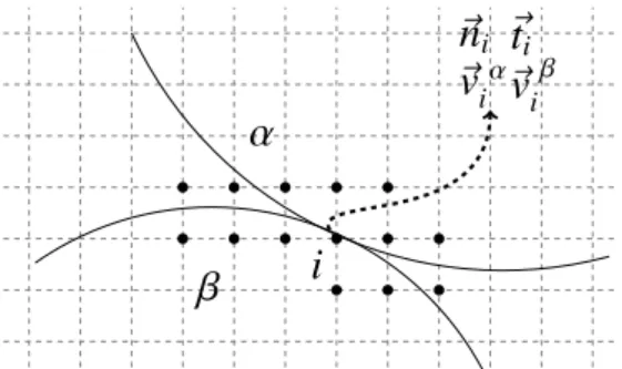
Fig. 1. Geometry of a contact between two soft particles discretised in multi-mesh MPM algorithm. The solid points represent the potential contact nodes; see text.

weak form of the equation of motion(2)in its discretised version can be written as follows by considering the contact interactions between several bodies [11]:

M anode(t)

=

fint(t)

+

fext(t)

+

fc(t)

,

(4)

where anodeis the nodal acceleration, fcdenotes the contact force,

which will be illustrated below, and M

=

Np

∑

p=1

mpNp lumped mass matrix,

fint(t)

= −

Np

∑

p=1

Gp

σp

(t) Vp(t) internal force vector,

fext(t)

=

Np

∑

p=1

Npbp(t)

+

fs(t) sum of body forces and

surface tractions fs

.

In the above relations, Vpdenotes the material point volume and

Np is the interpolation matrix or the shape function matrix at

a material point p. It relates the quantities associated with the material points (displacement, position

· · ·

) to nodal variables of the element to which the material point belongs. Gpdenotes the

gradient of the shape function Np.

Since there are generally more material points than grid nodes, a weighted squares approach is used to determine nodal velocities vnodefrom the material point velocities vp. Hence, the nodal

veloc-ities are obtained by solving the relation Pnode(t)

=

M vnode(t)

=

∑N

p

p=1mpNpvp(t)

,

(5)

where Pnodeis the nodal momentum.

It is also important to note that, as we deal with deformable particle systems, the contact forces fcbetween particles need to be

computed using a contact algorithm that accounts for the condition of impenetrability of matter as well as the Coulomb friction law. This contact algorithm combines the MPM and CD methods that was presented in detail in our previous paper [11]. For clarity, in the following, we briefly describe this algorithm.

Let us consider two deformable particles (

α

and

β

); seeFig. 1. In the context of the multi-mesh algorithm, a proper background mesh is attributed to each particle. A contact point at the interface between the two particles may be treated by introducing a com-mon background mesh with the same type of grids for the transfer of nodal quantities from the proper meshes to the common mesh. The contact points between the particles

α

and

β

are treated at the neighbouring nodes belonging to the common background mesh. Their nodal values involve contributions from the two particles. At a potential contact node i, a normal unit vector ni, oriented

from particle

β

to particle

α

, and a tangential unit vector ti are

Fig. 2. Contact conditions: (a) Velocity-Signorini complementarity condition as a graph relating the normal relative velocityvnand normal force fn; (b) Coulomb friction law as a graph relating the tangential velocityvtand friction force ft;µis the coefficient of friction. The dashed lines represent the linear relations obtained from a linear combination of the equations of dynamics; see text.

remains positive, the normal force fnis identically zero. But when

vn

=

0, a non-negative (repulsive) normal force fnis mobilised at

the contact node. These conditions define the velocity-Signorini complementary condition as shown in Fig. 2(a) [19,20]. On the other hand, by combining the equations of motion Pα_node

=

Mαvα_node and Pβ_node

=

Mβvβ_nodeat the common node i, we get the following linear relation:

fn

=

_∆1t mα_i mβ_i

mα_i+mβ_i

vn

+

kn

,

(6)

where mα_i and mβ_i are the nodal masses of bodies of

α

and

β

, respectively,∆t denotes the incremental time, and knis an offset

force which depends on other contact forces exerted by the neigh-bouring bodies of

α

and

β

. The normal force at all contact nodes are obtained through an iterative process by intersecting the above linear relation with the Signorini graph, as shown inFig. 2(a).

In a similar vein, the Coulomb law of dry friction is a comple-mentarity relation between the friction force ftand the tangential

velocity

vt

(

vt

=

(vα_i

−

vβ_i)

·

ti) at the contact node; seeFig. 2(b).

Like the Signorini graph, the Coulomb law is a complementarity relation in the sense that it cannot be reduced to a single-valued function. The equations of motion at the common node i yield

ft

=

_∆1_t mα_i mβ_i

mα_i+mβ_i

vt

+

kt

,

(7)

which is intersected with the Coulomb graph to calculate the friction force ft simultaneously at all contact nodes in the same

iterative process used to calculate the normal forces. The conver-gence to the solution both for contact forces and internal stresses is smooth, and a high precision may be achieved through the convergence criterion.

It is worth noting that in the presented algorithm, a contact may occur between the particles even if they are not physically in contact. Indeed, since the contact is computed on the nodes of the background mesh (not on the material points), the distance between the particles in contact can vary within one element size. The contact force accuracy depends hence on the particle discretisation as well as time discretisation (time step). This issue exists in all contact algorithms and depending on the necessary solution accuracy required for a specified problem, one can adjust the time and/or space resolution. In our case, the proposed contact algorithm allows us to treat rapidly and accurately enough the contact between deformable particles with any arbitrary shape although some local parameters such as contact surface may not be accurately defined.

3. A finite strain formulation for MPM

To complement the continuity equation(1)and the momentum equation(2), we consider a constitutive relationship in the context

of the finite strain theory:

t

0Π(

0_x

_,

_t)

₌

_F(r)₍t

0F(

0_x

_,

_t))

_,

₍₈₎

wheret₀Π(0x

,

t) is the first Piola–Kirchhoff stress tensor at

posi-tion0x in the initial configuration and at time t. Lett₀F(0x

,

t)

=

∇

0_xu(tx

,

t)

+

I be the deformation gradient tensor, where I is the

second-order identity tensor. Note thatt₀Πandt₀F are defined at the actual configuration ‘t’ with respect to the initial configuration at time t

=

0.t

σ

is also related tot₀Πthrough

t

_σ

₍t_x

_,

_t)

₌

1 0_J t 0Π( 0_x

_,

_{t) (}t 0F( 0_x

_,

_t))T

_,

(9) with0_J

₌

_det(t

0F(0x

,

t) ). Note that, by virtue of the definition of the

constitutive relation(8), this framework corresponds to the finite strain theory, and it is not specifically designed for a particular constitutive law. Hence, the material behaviour can cover various nonlinear and complex physical and geometrical evolutions of the continuum body.

4. Finite strain MPM: an implicit-type formalism

In our previous paper [11], a MPM algorithm with an implicit time integration was introduced. In this section, we adopt this approach to our new formulation in the framework of the finite strain theory. Note that the implicit resolution concerns only the nodal parameters whereas those related to the material points are determined explicitly.

Let us advance the solution of(4)from ‘t’ to ‘t

+

∆t’ in the

context of the implicit resolution. We consider that fext(t

+

∆t)

is known, and the grid kinematics is advanced in time as follows: unode(t

+

∆t)

=

∆t vnode(t

+

∆t)

,

(10)

vnode(t

+

∆t)

=

vnode(t)

+

∆t anode(t

+

∆t)

.

(11)

Note that, in Eq.(10), we have unode(t)

=

0 since unode(t

+

∆t)

is in fact the grid displacement from ‘t’ to ‘t

+

∆t’. From Eqs.(10) and(11), the nodal acceleration at time t

+

∆t is given by

anode(t

+

∆t)

=

1

∆t2 unode(t

+

∆t)

−

1

∆t vnode(t)

.

(12)

In the context of the finite strain theory, the evaluation of the material point volume Vpchanges from t to t

+

∆t according to

Vp(t

+

∆t)

=

tJpVp(t) (13)

withtJ

=

det(t_t+∆tF ).

In an incremental-iterative resolution algorithm, a new esti-mation of the nodal displacement uk

node(t

+

∆t) at iteration k is

obtained by adding the incremental displacement∆uk

node to the

previous estimated displacement:

uk_node(t

+

∆t)

=

u_nodek−1(t

+

∆t)

+

∆uk_node

.

(14) To obtain∆uk_nodeat iteration k, we solve

Kk−1_∆uk

node

=

Rk

,

(15)

where K is the stiffness matrix and R refers to the residual term. This equation is the incremental form of relation(4). The terms K and R are defined inAppendix A.

This incremental algorithm finds a nodal displacement unode(t

+

∆t) that minimises the residual term, R. So, as in [21], we introduce two convergence criteria:

C1

=

∥∆uk_node∥ ∥∆umax node∥

< ϵ

1 and C2

=

∥∆uk_nodeRk∥ ∥_∆u1_nodeR1∥

< ϵ

2

,

(16)

where

ϵ

1and

ϵ

2are tolerance parameters on velocities and energy,

respectively,

∥ · ∥

is the norm operator,

∥

∆umax

node

∥

denotes the

maximum value of the norm of the incremental displacement, and

∥

∆u1

nodeR1

∥

indicates the initial value of the inner product of the

Fig. 3. Scheme of the parallelisation procedure of the MPM-CD framework; N is the number of the particles and, fc, m, n and t represent the contact force, mass, normal and tangential vectors, respectively, for the potential contact nodes of each particle.

5. MPM and parallel computation

The MPM simulations involving a modest number of particles and material points can be performed in a reasonable time on a single-processor workstation. As the number of particles and phys-ical complexity of the numerphys-ical model increase, so does the com-putational resources required. The simulation of 1000 particles, for example, with a sufficient number of material points for their discretisation is not thus suited to a single processor. Hopefully, the required level of computational power can be obtained by parallel MPM simulations. Herein, the goal is to produce a portable parallel implementation that would exhibit good performance scaling up to several hundred processors for large-scale simulations. The code is required to run on parallel computer systems having either shared or distributed memory.

5.1. Parallelisation procedure

The proposed MPM parallel algorithm is of SPMD (Single Pro-gram, Multiple Data) style, based on MPI. The particles in the simulation domain are divided into spatial sub-domains. Choosing the number of sub-domains equal to the number of available pro-cessors, the data associated with particles in the same sub-domain are stored in the memory of a single processor. The computational effort depends on the resolution of Eq.(4)for each particle, which is closely related to the particle volume. Assuming that the pro-cessors have equal performances, to achieve load balance (needed to minimise synchronisation delays), the sub-domains should be chosen such that the sum of volumes of particles is nearly the same in all sub-domains. Hence, the particles in a sub-domain are not necessarily neighbours.

In the proposed MPM algorithm, the resolution of Eq.(4) im-poses the computation of the contact forces fc for each particle,

which depend on the interactions between particles. Since the contact forces are computed on the master process, the only data exchange between the particles (and thus the processors) are the contact forces fc; seeFig. 3. It is also worth noting that the

computation of contact forces on the master process is constant independently of the number of processors and represents less than about 0.5% of the total computational time.

5.2. Load balance

Each MPI thread manages MPM computations of a set of par-ticles, one particle being attributed to only one process. So, the

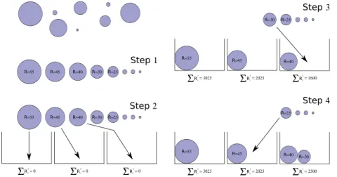
elementary MPM computational weight unit is the weight of a particle. However, particles involved in the global simulation do not exhibit exactly the same volume, and thus the same compu-tational weight. To reach correct performances, the particles have to be distributed in such a way that the weight is well balanced between processes. To do so, we propose the following algorithm for P processes:

1. The N particles are sorted by decreasing radius.

2. The P largest sorted particles are attributed to the P pro-cesses.

3. The P

+

1 particle is attributed to the process with the lightest workload

4. Step 3 is iterated until all particles are attributed.

Fig. 4displays our load balance algorithm for an example of circular particles in 2D. As the weight here is proportional to the particle surface (in 2D), the total surface of particles

∑

Ri2must

be well balanced. This approach allows reaching very low load imbalances. For instance, it is less than 1% for N

=

300 particles (radii of particles ranging from 0.7 mm to 1.2 mm) and P

=

60 processes.

5.3. Scalability

The scalability of the code was studied with the help of the cluster of the Genotoul Bioinformatics Platform (Toulouse, France). Each compute node embeds 2 Ivy-Bridge 10 cores hyper-threaded microprocessors (2

.

5 GHz) and the nodes are interconnected through a QDR Infini-Band network for both MPI communications and IO. In our study, the number of processors P varies from 1 to 60, and according to this number at most 20 cores were used per compute node.

As shown inFig. 5, the scaling is not linear and the efficiency decreases quite fast when P increases. Clearly, such a behaviour can be attributed to the communication bottleneck in rank 0 process. Collective communications involved in data exchange between MPM and Contact Dynamics lead to a large amount of data to be sent or received by rank 0 MPI thread. Such a point should be addressed in future improvements of our code.

6. Numerical examples

The accuracy and efficiency of the proposed algorithm within the finite strain theory are studied through several mechanical compaction tests. In our previous works [11,12], the performance of a similar approach in the framework of the infinitesimal strain hypothesis was shown. We propose two main applications. The first one deals with the uni-axial deformation of a single soft particle. The second example concerns the compaction of a packing of 300 soft particles. To avoid stress gradients in these examples, the gravitational acceleration is set to be zero.

In the MPM, two-dimensional simulations in plane strain con-ditions were performed. The computation domain was meshed with four-node quadrangular elements. For the applications that we target in the present work, we consider two types of material behaviours [14]: a linear Saint-Venant Kirchhoff constitutive rela-tion

S

=

λ

Tr(

γ

) I

+

µ γ ,

(17)

and a nonlinear Neo-Hookean constitutive law

S

=

(

λ

ln(J)

−

µ

) C−1

+

µ

I

,

(18) where S is the second Piola–Kirchhoff stress tensor and related toΠthrough Π

=

F S. Let C

=

FT_{F be the right symmetric}

Cauchy–Green tensor.

γ

denotes the Green–Lagrange strain tensor (

γ =

1₂(C

−

I)) and J

=

det (F).

λ

and

µ

represent the Lamé coefficients.

Fig. 4. Load balance algorithm. A set of circular particles (in 2D) is shown, Ri2_{being written in each particle, and distributed in 3 processes. The total workload}∑

Ri2is updated at each step.

Fig. 5. Measured speedup for the MPM-CD simulation of 300 particles. The line represents perfect scaling.

Fig. 6. Contact geometry between a single particle and a rigid plate.

6.1. Axial compaction of a single particle

We consider here the case of a single cylindrical particle sub-jected to axial compression. The particle has a diameter of D

=

20 mm and is compressed between two rigid walls as shown in Fig. 6. The bottom wall is fixed and the top wall moves downwards at a constant velocity of 0

.

5 m

/

s. The time step is set to∆t

=

Fig. 7. Normal contact force applied on a single particle as a function of the displacement of the particle centre for two different behaviours.

0

.

1

µ

s. To compare the infinitesimal and finite strain formulations in the context of the MPM, the linear Hookean and Saint-Venant Kirchhoff elastic behaviours (see Eq.(17)) are considered. In the two cases, the Lamé coefficients and density of the particles were set to

λ =

100 MPa,

µ =

1

.

5 MPa and

ρ =

990 kg

/

m3_,

respectively.Fig. 7presents the normal contact force F as a function of displacement d of the centre of the particle. In the two cases, a quasi-linear evolution of force with displacement is observed but with a small deviation ford_D

>

0

.

05 towards a lower level of force. This behaviour corresponds to the prediction of the Hertz analysis for a cylinder of unit length [22]:

F

=

π₄E∗

d

,

(19)

where E∗is the effective elastic modulus defined as E∗

=

E

/

(1

−

ν

2) with E being Young’s modulus and

ν

Poisson’s ratio. Furthermore, the predicted values of forces by the infinitesimal and finite strain formulations are not very different. This means that, as a result of the small value of the time step, the second order terms in the Green–Lagrange strain rate have little effect on the total strain.

We carried out the same test by considering a Neo-Hookean particle (see Eq.(18)). We set

µ =

1

.

5 MPa,

ρ =

990 kg

/

m3_,

and three values of

λ =

0, 3 and 100 MPa. These different values of

λ

define the compressibility of the particle, i.e. for

λ =

0 the particle is fully compressible whereas for

λ =

100 MPa the particle

Fig. 8. Geometry of a single Neo-Hookean particle and it’s deformed configurations at vertical strainγyy=20% for different values ofλ. Although the deformed particles seem to touch the two walls only over a short segment at the centre, the material points belonging to the boundary elements between the particle and the bottom and top walls are actually within the contact zone. The observed gap is due to the background mesh element thickness.

Fig. 9. The stress–strain diagrams for a single Neo-Hookean particle subjected to diametrical compression for several values ofλ.

is quasi-incompressible. The deformed particles at vertical strain

γyy

=

20% for these values of

λ

are shown inFig. 8.

We also note the decrease of the lateral extension as the particle compressibility increases. This extension is negligible for the fully compressible particle (

λ =

0 MPa) (seeFig. 8). It can be explained by the fact that for the incompressible particle, the volume of the compressed portion can migrate to the non-contact portion more efficiently as a result of its dense structure [23]. Fig. 9displays the second Piola–Kirchhoff stress Syyas a function of the Green–

Lagrange strain

γyy

. We see that the stress increases as

λ

increases. In other words, deforming less compressible particles requires a larger force.

6.2. Compaction of a packing of elastic particles

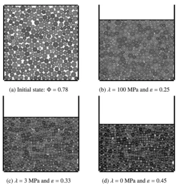
In this section, we investigate the compaction of a packing of elastic particles using the Neo-Hookean material behaviour. By means of MPM simulations, we study the evolution of different packing properties (packing fraction, connectivity etc.). We con-sider a packing of 300 particles confined inside a rectangular box. The initial configuration is prepared by means of DEM simula-tions. A uniform distribution of the particle diameters by volume fractions in the range

[

2

,

4

]

mm is introduced. This polydispersity allows avoiding long-range ordering. We simulate the compaction process by moving the top wall downwards at constant velocity

Fig. 10. A snapshot of the initial configuration (a) and three snapshots of the compaction of a packing of soft particles with Neo-Hookean behaviour for packing fraction of 0.97 and several values of theλ(b–d). Note that, despite the same value of the packing fraction, the packing volumes are different due to the different compressibilities of the particles. The black points represent the material points.

of 2 m

/

s and with a time step of∆t

=

0

.

1

µ

s. We consider the Neo-Hookean particles with the same material parameters as in the previous section. The gravitational acceleration is set to be zero in order to avoid stress gradients. There is no friction between the particles, and between the particles and the walls.

Fig. 10 represents the snapshots of the compaction test for different values of

λ

. The packing fractionΦ

=

VS/V , where VS

is the volume of particles and V the total volume, increases by particle shape change and at the end of the compaction nearly the whole space is filled by the particles. The shapes of the particles gradually change from circular to nearly polygonal as shown in Fig. 10. Note that the gaps observed between particles are related to the meshing resolution, which may be increased for a finer discretisation of the contact zone. Moreover, as mentioned before, since the less compressible particles can elongate more, the pores between these particles are more rapidly filled even for a low global deformation.

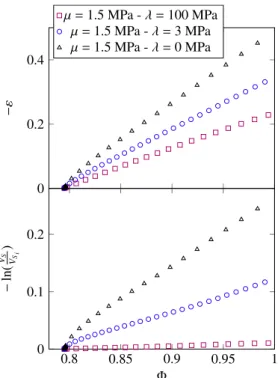
The above feature is more clearly highlighted inFig. 11. It shows the cumulative volume deformation of the particles defined by ln(VS

/

VSi), where VSiis the initial volume of the particles, and the

cumulative vertical strain

ε

as a function of the packing fractionΦ. The latter is expected to vary due to the elastic volume change of the particles as a result of elastic compressibility of the particles as well as the variation of the total volume V due to particle rearrangements and shape change. Since the width of the box is constant, we have ln

(

VS V_Si

)

=

ln

(

Φ Φi

)

+

ε

(20)

with

ε =

ln(h

/

hi), where hiis the initial height of the sample. In

Fig. 11, the data for three values of

λ

coincide up to Φ

≃

0

.

8. Beyond this packing fraction,

ε

and ln(VS

/

VSi) vary at different

nearly linear rates for each

λ

value. As expected, this rate increases as

λ

(or compressibility) decreases. Note that for

λ =

100 MPa (quasi-incompressible particles), the volume variation of particles is negligibly small as shown inFig. 11. Moreover, one can consider

Fig. 11. Evolution of the cumulative vertical strainεand, the total particles volume change ln(VS/VSi) as a function of the packing fractionΦfor several values ofλ.

Fig. 12. Evolution of the excess mean coordination number Z−Z0as a function of

excess packing fractionΦ − Φ0for several values ofλ. The solid line is power-law fit (Φ − Φ0)0.5_{; see Eq.(21).}

Φ

≃

0

.

8 as the jamming point above which no particle rearrange-ments occur anymore, and thus the packing evolution is only due to particle shape change.

The mean coordination number Z is an important parameter, which evolves with the evolution of the packings.Fig. 12displays

Z as a function ofΦ. We see that by normalising the excess coordi-nation number Z

−

Z0, where Z0is the mean coordination number at

the jamming point, by Z1

−

Z0, where Z1is the coordination number

atΦ1

≃

1, andΦ

−

Φ0byΦ1

−

Φ0, all data points collapse on a

single plot that is well fitted by a power-law function:

Z−Z0 Z1−Z0

=

(

_Φ−Φ 0 Φ1−Φ0

)

0.5

.

(21)

A similar power-law behaviour was observed by several authors specially in the case of emulsions and foams [17,24,25] in the following form:

Z

−

Z0

=

z0(Φ

−

Φ0)β

.

(22)

Fig. 13. The normalised applied stress as a function of packing fraction normalised by the particle P-wave modulus Mpfor several values ofλ. The lines represent the predicted behaviour by the model of compaction introduced in this paper; see Eq.(23).

These two last equations coincide by setting

β =

0

.

5 and

z0

=

(Z1

−

Z0)

/

(Φ1

−

Φ0)0.5. As in our study, for all cases, we have

Z0

≃

4 forΦ0and Z1

≃

5

.

6 forΦ1, one gets z0

≃

3.6. This value

is fully consistent with O’Haren et al. (2003) [24] who predicted that z0is equal to 3.5

±

0.3 and

β ≃

0

.

5

±

0.03 in 2D. It is also

interesting to note that the material behaviour of the particles has almost no effect on these results (seeFig. 12), in agreement with the references [17,24,25], which observed that the evolution of the coordination number with packing fraction is independent of space dimension, interaction potential and polydispersity.

The evolution of the applied stress

σ

beyond the jamming point allows for a macroscopic analysis of the packing evolution.Fig. 13 shows

σ

, computed from the contact forces acting on the bottom wall and normalised by the particle P-wave modulus Mp(Mp

=

λ+

2

µ

) as a function ofΦ. We note a nonlinear behaviour for three cases with different rates. As in the case of one particle simulations, we observe also that the required force to compress the packing in-creases with the particle compressibility. These observations may be explained by the fact that beyond the jamming point the packing behaves almost like a continuum medium as there are no more particle rearrangements. This assumption leads to a logarithmic relation between

σ

andΦ(seeAppendix B):

σ MP

= −

ZΦ Z+Mp c1Kp (ln(Φ)

+

c2)

,

₍₂₃₎

where Kpis the particle bulk modulus (Kp

=

λ + µ

in 2D), c1is

a parameter depending on the particle material behaviour and c2

is a constant term. The coordination number Z is also defined as a function ofΦby Eq.(21). The predictions of this model(23)are in good agreement with our MPM simulations shown inFig. 13with

c2

≃

0

.

27, and c1

≃

0

.

01 for

λ =

100 MPa, c1

≃

0

.

23 for

λ =

3 MPa and c1

≃

1

.

3 for

λ =

0 MPa. Note that, although this model

seems to predict well the applied stress

σ

as a function ofΦ, at high packing fractions, the Neo-Hookean particles can only overfill the remained little pores for much higher stresses (involving smaller and smaller radii of curvature) but when the packing fraction tends to 1, the corresponding applied stress should tend to infinity. Hence, this model does not hold at high values of the packing fraction. In our simulations, to resolve correctly the small radii of curvature at the contact zones between particles, one should refine in the same proportion the discretisation.

In order to analyse the particle deformations and volume change during the compaction of the packings, we also consider the evo-lution of the distribution of the equivalent von Mises strain

γeq

and

Fig. 14. Evolution of the standard deviation SD and excess Kurtosis exKurt of the equivalent von Mises strain,γeqas a function of the packing fractionΦfor several values ofλ.

Fig. 15. Evolution of the standard deviation SD and the excess Kurtosis exKurt of0_J

as a function of the packing fractionΦfor several values ofλ.

the Jacobian of deformation gradient0_{J (see Eq.(9)), respectively.}

Here,

γeq

is defined as

γeq

=

√

2

3

γ

d

:

γ

d

,

(24)

with

γ

d

₌

_{γ −}

1

3 Trace(

γ

) I. To characterise the shapes of these

distributions, we consider here their standard deviation and excess kurtosis.Fig. 14displays the standard deviation and excess kurtosis

of

γeq

as a function ofΦ. The standard deviation of

γeq

for the three values of

λ

coincide up toΦ

≃

0

.

8, but beyond this value they vary at different rates. In the quasi-incompressible case (

λ =

100 MPa), the standard deviation is larger than in compressible cases. This trend can be explained by the occurrence of more important stress chains between particles when their compressibility decreases. The values of the excess kurtosis of

γeq

distributions for several values of

λ

coincide, and they tend to a positive value about 2 beyond the jamming point. This value is compatible with a Lep-tokurtic distribution, which shows heavier tails than the normal distribution.

Finally, the standard deviation and the excess kurtosis of the Jacobian of deformation gradient0_{J as a function ofΦare shown}

inFig. 15. As expected, the standard deviation for

λ =

100 MPa (quasi-incompressible particles) is almost zero since there is no particle volume change. The standard deviation is larger for the fully compressible particles (

λ =

0 MPa). It is due to the larger possible deformation of the particles in this case. However, the kurtosis is nearly zero, meaning that the0_{J distributions are nearly}

normal. 7. Conclusion

In this paper, we improved our approach for modelling soft-particle systems developed in [11]. In this novel approach, the finite strain formulation is used in the context of the implicit Material Point Method (MPM). The MPM allows one to take into account the realistic mechanical behaviour of individual particles. Coupling the MPM with the Contact Dynamics (CD) method makes it possible to deal correctly with frictional contacts between parti-cles.

It was shown that two MPM formulations (infinitesimal and finite strain) are similar. The finite-strain formulations can host more complex constitutive behaviours such as hyperelasticity for the particles. Furthermore, to improve computational performance, a parallelisation procedure was proposed in the framework of this algorithm. Although the efficiency of this proce-dure declines with increasing number of processors, it is still useful for decreasing the computational cost.

The uni-axial compaction of a packing of soft particles was simulated using MPM by considering several values of particle compressibility (from quasi-incompressible to fully compressible particles). The packing with more compressible particles can un-dergo larger deformations under the action of lower compressive stress due to considerable particle volume changes and occur-rence of weaker stress chains between particles. It was shown that this stress beyond the jamming state varies logarithmically with packing fraction. This behaviour was explained by introducing a simple model. Another interesting result of this work concerns the evolution of the coordination number, which can be related to the packing fraction by a power-law function beyond jamming transition.

Acknowledgements

This work/project (ID 1502-607) was publicly funded through ANR (the French National Research Agency) under the ‘‘Investisse-ments d’avenir’’ programme with the reference ANR-10-LABX-001-01 Labex Agro and coordinated by Agropolis Fondation, France under the frame of I-SITE MUSE (ANR-16-IDEX-0006). We are also grateful to the genotoul bioinformatics platform Toulouse Midi-Pyrenees (Bioinfo Genotoul) for providing computing resources. Conflict of interest

Saeid Nezamabadi, Xavier Frank, Jean-Yves Delenne, Julien Averseng and Farhang Radjai state that there are no conflicts of interest.

Appendix A. Definitions of K and R

The implicit integration in the context of MPM takes into ac-count the discretised equation of the motion:

M anode(t

+

∆t)

=

fint(t

+

∆t)

+

fext(t

+

∆t)

,

(A.1)

By considering that the external force at time t

+

∆t is known,

fext(t

+

∆t), and by assuming an incremental-iterative Newton

solution strategy, the linearised equation of motion at iteration k is Kk−1_∆uk node

=

R k

_,

_(A.2) where Kk−1

=

1 ∆t2 M

−

Np

∑

p=1 Vp(t) Gp t +_∆t t H k−1 p Gp (A.3) Rk

₌

_f ext(t

+

∆t)

+

fk −1 int (t

+

∆t)

−

M a k−1 node(t

+

∆t)

,

(A.4) with t_J pt +∆t

_σp

₌

t+∆t t Hp t +∆t t Fp

.

Note that in the last relation,t+_∆t

Hpcan be obtained using Eq.(9)

and the constitutive relation(8).

Appendix B. Relation between the applied stress,

σ

, and the packing fraction,Φ, for a packing under uniaxial compression

We assume that the packing of particles behaves almost as a continuum medium beyond the jamming point under uniaxial compression. Hence, in this range the applied stress

σ

may be related to the cumulative vertical strain

ε

through an effective P-wave modulus M:

σ =

M

ε .

(B.1)

Here, the particle and pore volume changes can be assumed to be the same, implying that the effective P-wave modulus is propor-tional to the packing fraction: M

=

ΦMp with Mp the particle

P-wave modulus. One may further assume that the particle bulk modulus Kprelates the volume increment dVS of particles to the

effective stress increment d

σS

in particles:

KpdV_VSS

= −

d

σS

.

(B.2)

σ

can be related to

σS

as follows:

σ =

c1ZΦ

σS

,

(B.3)

where c1 is a material constant to determine. Given that d

ε =

dVS

/

VS

−

dΦ

/

Φand using Eqs.(B.1),(B.2)and(B.3), the following

differential equation to solve is obtained: (Z

+

_cMp 1Kp)d

σ =

[

(Z

+

_cMp 1Kp) σ Φ

−

MpZ

]

dΦ

+

_cMp 1Kp σ ZdZ

,

(B.4)

By knowing that there is a relationship between Z and Φ (see Eq.(21)), the integration of the differential equation(B.4)is given:

σ MP

= −

ZΦ Z+Mp c1Kp (ln(Φ)

+

c2)

,

_(B.5)

where c2is the integral constant.

References

[1] P.A. Cundall, O.D.L. Strack, Géotechnique 29 (1979) 47–65.

[2] H. Matuttis, S. Luding, H. Herrmann, Powder Technol. 109 (2000) 278–292.

[3] J. Moreau, Eur. J. Mech. A Solids 13 (1994) 93–114.

[4] M. Jean, F. Jourdan, B. Tathi, Proceeding of The International Deep Drawing Research Group (IDDRG 1994), in: Handbooks on Theory and Engineering Applications of Computational Methods, 1994.

[5] F. Radjai, V. Richefeu, Mech. Mater. 41 (2009) 715–728.

[6] F. Da Cruz, F. Chevoir, D. Bonn, P. Coussot, Phys. Rev. E 66 (2002) 051305.

[7] M. Cloitre, R. Borrega, F. Monti, L. L., Phys. Rev. Lett. 90 (2003) 068303.

[8] R. Bonnecaze, M. Cloitre, Adv. Polym. Sci. 236 (2010) 117–161.

[9] A. Favier de Coulomb, M. Bouzid, P. Claudin, E. Clément, B. Andreotti, Phys. Rev. Fluids 2 (2017) 102301.

[10] M. Barnabe, N. Blanc, T. Chabin, J.-Y. Delenne, A. Duri, X. Frank, V. Hugouvieux, E. Lutton, F. Mabille, S. Nezamabadi, et al., Innovative Food Sci. Emerg. Tech-nol. (2017).

[11] S. Nezamabadi, F. Radjai, J. Averseng, J.-Y. Delenne, J. Mech. Phys. Solids 83 (2015) 72–87.

[12] S. Nezamabadi, T. Nguyen, J.-Y. Delenne, F. Radjai, Granular Matter 19 (2017) 8.

[13] V. Acary, B. Brogliato, Numerical Methods for Nonsmooth Dynamics. Applica-tions in Mechanics and Electronics, Springer, 2009.

[14] S. Nezamabadi, H. Zahrouni, J. Yvonnet, Comput. Mech. 47 (2011) 77–92.

[15] J.G. Berryman, Phys. Rev. A 27 (1986) 1053.

[16] S. Torquato, T.M. Truskett, P.G. Debenedetti, Phys. Rev. Lett. 84 (2000) 2064.

[17] M. van Hecke, J. Phys.: Condens. Matter 22 (2010) 033101.

[18] P. Huang, X. Zhang, S. Ma, X. Huang, Internat. J. Numer. Methods Engrg. 85 (2011) 498–517.

[19] M. Jean, in: A. Salvadurai, J. Boulon (Eds.), Mechanics of Geomaterial Inter-faces, Elsevier Science Publisher, Amsterdam, 1995, pp. 463–486.

[20] B. Brogliato, Nonsmooth Mechanics, Springer, London, 1999.

[21] J. Guilkey, J. Weiss, Internat. J. Numer. Methods Engrg. 57 (2003) 1323–1338.

[22] K. Johnson, Contact Mechanics, Cambridge University Press, Cambridge, 1999.

[23] Y.-L. Lin, D.-M. Wang, W.-M. Lu, Y.-S. Lin, K.-L. Tung, Chem. Eng. Sci. 63 (2008) 195–203.

[24] C. O’Hern, L. Silbert, A. Liu, S. Nagel, Phys. Rev. E 68 (2003) 011306.

[25] J. Zhang, T.S. Majmudar, M. Sperl, R. Behringer, Soft Matter 6 (2010) 2982–2991.