Publisher’s version / Version de l'éditeur:
Vous avez des questions? Nous pouvons vous aider. Pour communiquer directement avec un auteur, consultez la
première page de la revue dans laquelle son article a été publié afin de trouver ses coordonnées. Si vous n’arrivez pas à les repérer, communiquez avec nous à [email protected].
Questions? Contact the NRC Publications Archive team at
[email protected]. If you wish to email the authors directly, please see the first page of the publication for their contact information.
https://publications-cnrc.canada.ca/fra/droits
L’accès à ce site Web et l’utilisation de son contenu sont assujettis aux conditions présentées dans le site
LISEZ CES CONDITIONS ATTENTIVEMENT AVANT D’UTILISER CE SITE WEB.
New Journal of Physics, 21, 9, pp. 1-15, 2019-09-10
READ THESE TERMS AND CONDITIONS CAREFULLY BEFORE USING THIS WEBSITE.
https://nrc-publications.canada.ca/eng/copyright
NRC Publications Archive Record / Notice des Archives des publications du CNRC :
https://nrc-publications.canada.ca/eng/view/object/?id=736823b0-d1b3-4e69-b71a-7fa96089be43
https://publications-cnrc.canada.ca/fra/voir/objet/?id=736823b0-d1b3-4e69-b71a-7fa96089be43
NRC Publications Archive
Archives des publications du CNRC
This publication could be one of several versions: author’s original, accepted manuscript or the publisher’s version. / La version de cette publication peut être l’une des suivantes : la version prépublication de l’auteur, la version acceptée du manuscrit ou la version de l’éditeur.
For the publisher’s version, please access the DOI link below./ Pour consulter la version de l’éditeur, utilisez le lien DOI ci-dessous.
https://doi.org/10.1088/1367-2630/ab3d97
Access and use of this website and the material on it are subject to the Terms and Conditions set forth at
Realistic sub-Rayleigh imaging with phase-sensitive measurements
Bonsma-Fisher, Kent A. G.; Tham, Weng-Kian; Ferretti, Hugo; Steinberg,
Aephraim M.
PAPER • OPEN ACCESS
Realistic sub-Rayleigh imaging with
phase-sensitive measurements
To cite this article: Kent A G Bonsma-Fisher et al 2019 New J. Phys. 21 093010
View the article online for updates and enhancements.
Recent citations
Quantum Semiparametric Estimation Mankei Tsang et al
-Photonic quantum metrology Emanuele Polino et al
-Resolving starlight: a quantum perspective Mankei Tsang
New J. Phys. 21(2019) 093010 https://doi.org/10.1088/1367-2630/ab3d97
PAPER
Realistic sub-Rayleigh imaging with phase-sensitive measurements
Kent A G Bonsma-Fisher1,2,4 , Weng-Kian Tham1, Hugo Ferretti1and Aephraim M Steinberg1,3
1 Centre for Quantum Information & Quantum Control, Department of Physics, University of Toronto, 60 St. George St, Toronto, M5S
1A7, Canada
2 National Research Council of Canada, 100 Sussex Drive, Ottawa, K1A 0R6, Canada 3 Canadian Institute For Advanced Research, 180 Dundas St.W., Toronto, M5G 1Z8, Canada 4 Author to whom any correspondence should be addressed.
E-mail:kent.bonsma-fi[email protected][email protected]
Keywords: imaging, sub-Rayleigh imaging, Rayleigh’s curse, quantum information
Abstract
As the separation between two emitters is decreased below the Rayleigh limit, the information that can
be gained about their separation using traditional imaging techniques, photon counting in the image
plane, reduces to nil. Assuming the sources are of equal intensity, Rayleigh’s ‘curse’ can be alleviated by
making phase-sensitive measurements in the image plane. However, with unequal and unknown
intensities the curse returns regardless of the measurement, though the ideal scheme would still
outperform image plane counting
(IPC), i.e. recording intensities on a screen. We analyze the limits of
the super-resolved position localization by inversion of coherence along an edge
(SPLICE) phase
measurement scheme as the intensity imbalance between the emitters grows. We
find that SPLICE still
outperforms IPC for moderately disparate intensities. For larger intensity imbalances we propose a
hybrid of IPC and SPLICE, which we call
‘adapted SPLICE’, requiring only simple modifications.
Using Monte Carlo simulation, we identify regions
(emitter brightness, separation, intensity
imbalance) where it is advantageous to use SPLICE over IPC, and when to switch to the adapted
SPLICE measurement. We
find that adapted SPLICE can outperform IPC for large intensity
imbalances, e.g. 10 000:1, with the advantage growing with greater disparity between the two
intensities. Finally, we also propose additional phase measurements for estimating the statistical
moments of more complex source distributions. Our results are promising for implementing phase
measurements in sub-Rayleigh imaging tasks such as exoplanet detection.
1. Introduction
Rayleigh’s criterion places a limit on resolving closely-separated objects [1]. As the separation between two
incoherent point sources becomes smaller, image plane counting(IPC) measurements break down. More explicitly, the uncertainty in any unbiased estimation of the separation diverges as the separation is decreased below the Rayleigh criterion, which is given by the width of their point spread functions(PSF). Recently, strategies have emerged which beat Rayleigh’s criterion by using phase information of the two incoherent electromagneticfields in the image plane, information which is not available when using IPC [2–8]. This phase
information allows for the distance between two equal-intensity sources to be estimated withfinite variance even as their separation becomes arbitrarily small. For a Gaussian PSF, one way to access this phase amounts to making projective measurements in the Hermite–Gauss (HG) position basis. A recent flurry of experimental works have used this technique to demonstrate an advantage over IPC. In these works the HG projective
measurements were performed in various ways including spatial light modulation[9], homodyne detection [10],
self-interference[11], or a phase mask followed by single-mode fiber coupling [12]. Further developments in
this rapidly-emergingfield have addressed the analogous problem in the spectro-temporal domain [13],
estimating the angular and axial separation of the two point sources[14], studying the two- [15] and three- [16]
dimensional cases, and by employing Hong-Ou-Mandel interference[17]. In light of these discoveries, scientists
have moved to modernize Rayleigh’s criterion [18,19].
OPEN ACCESS
RECEIVED 31 May 2019 REVISED 23 July 2019 ACCEPTED FOR PUBLICATION 21 August 2019 PUBLISHED 10 September 2019
Original content from this work may be used under the terms of theCreative Commons Attribution 3.0 licence.
Any further distribution of this work must maintain attribution to the author(s) and the title of the work, journal citation and DOI.
Until recently these works have assumed the intensities of the two point sources to be equal. It has been shown[20,21] that when this assumption is relaxed—the two sources have unknown, disparate intensities—
that the quantum Cramér–Rao bound (CRB) for an unbiased estimate of the separation diverges as separation decreases below the Rayleigh limit5. However, this divergence happens quadratically slower than the CRB for IPC, suggesting that measurement schemes exist which still give an advantage over directly imaging the sources. Any further information to be gained must then be in the phase of the incoming light.
In this work we show that the super-resolved position localization by inversion of coherence along an edge (SPLICE) measurement scheme, introduced in [12], can be adapted to estimate the separation of unequal
intensity sources. Wefirst outline where SPLICE finds an advantage over IPC for estimating the separation of equal-intensity emitters, asking what the lowest resolvable separation is with each technique. In the unequal intensity case wefind, somewhat surprisingly, that SPLICE can still resolve much lower separations than IPC, within a given error threshold, up until some critical intensity imbalance. Beyond that, SPLICE can be adapted with additional projective measurements. We outline these measurements to estimate the variance and skew of the spatial distribution of light from which both the separation and relative intensities can be calculated. We evaluate the performance of the scheme by looking at the CRB and also Monte Carlo simulations,finding that the adapted SPLICE technique can resolve lower separations than IPC for imbalanced intensities. Moreover, the gap between SPLICE and IPC only grows as the relative intensities between the emitters gets more extreme. Following work by Tsang[22], we also outline a series of SPLICE-inspired measurements to estimate up to the
tenth statistical moment for an arbitrary distribution of point sources.
2. Super-resolved position localization by inversion of coherence along an edge
(SPLICE)
We begin by reviewing the SPLICE measurement scheme introduced by Tham et al[12] for the case of equalintensity emitters. The SPLICE measurement approximates a projection on the HG10mode using a glass edge,
which induces aπ phase-shift on half of the transverse profile of the incoming light, followed by a single-mode fiber (see figures1and2). We consider two incoherent point sources separated by a distance δ along the x-axis.
Each source is transformed by a Gaussian PSF∣ (y x y, )∣2with widthσ, such that if an emitted photon is equally
likely to have come from either source it can be described by the density matrix
x y x y x y 1 2 1 2 , d d 2, , , 1 r y y y y y y d = + = + + - -
∬
-¥+¥ ∣ ⟩⟨ ∣ ∣ ⟩⟨ ∣ ∣ ⟩ ( / )∣ ⟩ ( ) where x y, 1 exp x y 2 2 4 2 2 2 y = -ps s +{
}
( ) . The SPLICE projection∣f ñ2 has the form
x y x x y 1 2 d d e sgn , . 2 x y 2 2 4 2 2 2 f ps = s -¥ +¥ - +
∬
∣ ⟩ ( )∣ ⟩ ( )The probability of a successful photon detection is p2 2 2
8 2 2 4 4 f r f
= á ∣ ∣ ñ » psd + ( )ds forδ=σ. The separation is then estimated bydˆSPL= 8ps2k N, where k is the number of photons detected in a given time interval with
an average incident photonflux N, i.e. ká ñ =Np2. With IPC, one records the transverse positions of N incident photons on a screen, which are drawn from the intensity distribution 1 x x
2
2 1
2
2
= ∣ ∣á y+ñ +∣ ∣ ∣á y-ñ∣. The separation can be estimated by subtractingσ2from the estimate of the variance,dˆIPC=2 ( ˆv -s2).
Our primary concern is to identify the lowest value ofδ that, using either SPLICE or IPC, can be estimated to within some root mean square(rms) error threshold. Throughout this work we choose an error threshold of δ/5. This is done by comparing the CRB for the two measurement techniques. The CRB, the mean-squared error for an unbiased estimator, for a projective phase measurement such as SPLICE is independent ofδ in the sub-diffraction regime. We stress that this is only true for the equal-intensity case. For SPLICE the CRB is
N 2ps2
, whereas for IPC the CRB is
N 8 4
2
s
d. These are plotted in the inset offigure3(a) along with the rms error ofdˆSPLand IPC
dˆ from Monte Carlo simulations(see appendixAfor details). For low N, neither the SPLICE nor IPC
estimator agrees with its respective CRB due to estimator bias. In the biased regime, the standard deviation of the SPLICE estimate is constant. This biased regime extends through0 <d2⪅8ps2 N, and becomes unbiased
approximately when the expected number of detected photons is 1. This is discussed further in appendixB. The standard deviation of the IPC estimate scales as N−1/4in the biased regime. The IPC biased regime extends through0<d4⪅64s4 N, and becomes unbiased approximately when the error in thevariance estimate
becomes smaller than(δ/2)2.
5
For low error tolerances(black dotted line in figure3(a) inset) it suffices to simplify our discussion to only the
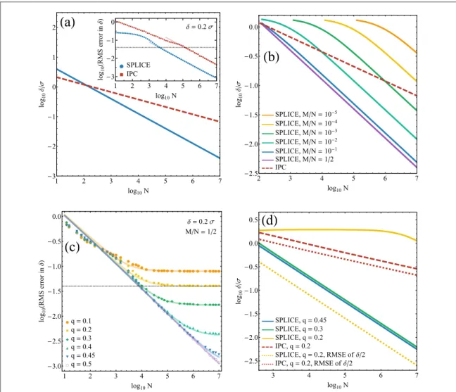
CRB scaling. That is to say, while in the biased regimes neither estimator will reach the desired error threshold. Infigure3(a) we plot the line where the square-root of the CRB is equal to an error tolerance of δ/5. This
represents the lowest resolvable separation for each measurement technique at a given source brightness N. For separationsδ<σ we see that SPLICE can resolve smaller separations than IPC. Importantly, the smallest separation resolved by SPLICE scales as N−1/2compared to a N−1/4scaling for IPC.
In a more realistic setting, the geometric center of the source distribution is not known a priori, and it is unclear of where to position the edge of the SPLICE phase-shifter. In[2], the authors analysed the setting where a binary
SPADE apparatus was aligned based on an initial IPC estimate. Here, we do the same for our(unadapted) SPLICE apparatus. As we will discuss in the next section, unequal intensities introduces the additional complication that even an IPC estimate of the geometric center is biased estimate from the true value. A goal of the present work is to identify how SPLICE compares to IPC in this scenario, and whether an adapted SPLICE measurement can yield an advantage over IPC. Before discussing this further, it is helpful to revisit the equal-intensity scenario where the geometric center is not known a priori. The strategy we consider is to estimate the mean position(x¯) of the intensity distribution using IPC, to which we align the SPLICE apparatus. A misalignment from the meanD = -m x¯ m1 affects the probability of a detection using SPLICE as p2
8 2 2 2 2 2 4 4 » psd + Dpsm +
( )
sd . The misalignmentΔμ is a normally distributed variable centered at 0 with varianceσ2/ M, where M is the number of photons used for mean estimation. We evaluate the estimatordˆSPLto compare with IPC, and infigure3(b) we plot the smallest separationthat can be estimated to within±δ/5 for both IPC and SPLICE. This is plotted for different fractions of the total photon input used for the mean estimation, M/N. The N−1/2scaling for resolving the lowest separation persists
using SPLICE but, due to poor estimation of the mean position at low photon numbers, the scaling does not start until large N. With larger fractions of photons allocated for mean estimation, the bias in the SPLICE measurement caused by misalignment is mitigated and the N−1/2scaling begins at lower values of N.
3. Unadapted SPLICE with unequal-intensity emitters
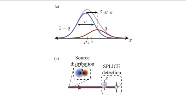
Relaxing the equal-intensity assumption, we have the scenario shown infigure1(a). The two emitters are
separated byδ about a center point c. A given photon with probability q of coming from the right emitter, and 1− q from the left, is described by the density operator
q 1 q . 3
r= ∣y+ñáy+∣+( - )∣y-ñáy-∣ ( )
There are now three unknown parameters,{δ, q, c}. It should be stated here that if c is known, one can align the SPLICE measurement about c and recover the same advantage as in the equal-intensity case. However, estimating c is not trivial since, when q¹1 2, c is no longer equal to the mean of the distribution and is offset
Figure 1.(a) The intensity distribution from two light sources separated by δ, much smaller than the PSF width σ. Due to unequal intensities, q and1 -q, the mean of the distribution,μ1, is displaced from the geometric center c.(b) The SPLICE detection scheme
for measuring the 2nd and 3rd moments along the x-axis uses a translatableπ-phase shifter and single-mode fiber.
from it by an amount related to the skew. The most naïve strategy is to align the SPLICE measurement about the mean, 1 c 1 2q
2
m = -( - )d, which is best estimated using IPC. Due to symmetry, for the rest of this work we
take 0q1/2.
With the SPLICE projection the same as in the previous section, the probability of a photon detection is now
p q q q q q q q O 1 2 2 1 1 2 3 1 2 1 2 . 4 2 2 2 2 2 3 4 2 2 2 2 4 4 f r f d ps d ps m d s m ps d s = = - + - - D +⎛ - - D + ⎝ ⎜ ⎞ ⎠ ⎟ ⎛ ⎝ ⎜ ⎞ ⎠ ⎟ ⟨ ∣ ∣ ⟩ ( ) ( )( ) ( ) ( )
The SPLICE estimator,dˆSPL = 8ps2k N, now includes more terms depending on q. When the misalignment
Δμ can be neglected, for example when N is large, the estimator returnsdˆSPL=2d q(1-q). Figure3(c) shows
the rms error fordˆSPLas a function of N whenδ=0.2σ for various values of q. We plot the results of Monte
Carlo simulations as well a numerically solved analytical expression(see appendicesAandBfor details). Note
that for these simulations we take half of the incident light to estimate the mean(M/N=1/2). We see that as the emitters deviate from equal intensity, q=1/2, the estimate results in a constant error at high N. This error comes from the fact that the SPLICE estimator explicitly depends on q, resulting in a bias ofd(1-2 q(1-q) ) at large N. For a given rms error thresholdò, there is a critical intensity value above which SPLICE can resolve separations with errorò. The critical intensity is qc 1 2
2 1 2
- = d - d
∣ ∣ ( ). For our chosen error threshold ò=δ/5 the critical value of qcis 1/5. This is outlined in figure3(d), where we again plot the lowest resolvable
separations for an error threshold ofδ/5. In the regime where SPLICE still functions, 1/5<q<1/2, it outperforms IPC: SPLICE has a N−1/2scaling compared to a N−1/4scaling for IPC. By allowing for bias in the SPLICE estimator it is still possible to reduce the rms error below the threshold. Given that the SPLICE
measurement was constructed with the assumption that the emitters are equally bright, is it somewhat surprising that SPLICE can still function at moderately disparate intensities. In the next section we discuss how the SPLICE measurement can be adapted for more extreme values of q.
4. Adapting SPLICE for unequal-intensity emitters
In the equal-intensity scenario the SPLICE measurement amounts to estimating the variance(2nd central moment) of the spatial distribution of the incident light, from which the separation can be calculated. After relaxing the equal-intensity assumption the variance no longer gives full information and, as one might expect fromfigure1(a), the
skew(3rd central moment) of the distribution becomes relevant. By translating the phase shifter and fiber transversely, with respect to the direction of light propagation, we can perform two additional measurements to estimate the skew. With estimates of the variance(m2=q(1-q)d2) and skew ( q 1 q 1 2q
3 3
m = ( - )( - )d), both
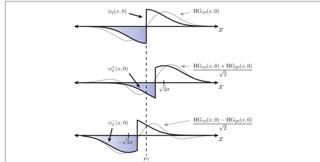
the separation(δ) and relative intensities (q) can be calculated. We introduce the projective measurements∣f ñ3 to estimateμ3. Higher moments of the source distribution can also be measured with additional phase shifters across
the transverse direction(see section5). The measurements for μ3are described by the projectors
x y x y x y x y x 1 2 d d , , , , e sgn 2 , 5 x y 3 2 3 3 2 4 2 2 2 f ps f f s = = ss -¥ +¥ - +
∬
∣ ⟩ ( )∣ ⟩ ( ) ( ) ( ) ( ) /which are, like∣f ñ2, realized by aπ phase-shifter and single-mode fiber coupler, each translatable along the x-axis. The∣f ñ3 projectors are constructed to approximate the iTEM projectors of[22], HG(∣ 10ñ ∣HG20ñ) 2 (see figure2). Expressing∣f ñ3 in the HG basis we have that
e e 2 HG HG 1 2 3 HG ..., 6 3 10 20 30 f p p ñ = ñ ñ + ñ ∣ (∣ ∣ ) ∣ ( ) x y x y x y x y m n x y HG d d HG , , , HG , He He 2 exp 4 , 7 mn mn mn m x n y 2 2 2 2 ps s = = s s - + -¥ +¥ ⎧ ⎨ ⎩ ⎫ ⎬ ⎭
( ) ( )
∬
∣ ⟩ ( )∣ ⟩ ( ) ! ! ( )whereHen( )x is the nth probabilists’ Hermite polynomial. For a Gaussian PSF the measurement success
probability HGá m0∣ ∣rHGn0ñis proportional to the n+mth statistical moment, μm+n, to leading order inδ/σ.
For the 2nd and 3rd moments we have thatm2µ áf r f2∣ ∣ 2ñ, andm3µ áf r f3+∣ ∣ +3ñ - áf r f-3∣ ∣ 3-ñ. In the latter case, theμ2andμ4terms are canceled in the subtraction. An interesting fact which emerges here is that the SPLICE
another position for the phase-shifter andfiber coupler which achieves higher overlap. However, making this choice also results in non-zero overlap with∣HG00ñ. This in turn gives a contribution fromμ1which does not
cancel in the subtraction and dominates over theμ3term. In constructing the SPLICE measurements it is crucial
to ensure zero overlap with all lower HG modes.
When the∣f ñ3 projectors are aligned with respect to x¯, misaligned from the mean byD = -m x¯ m1, the probabilities of photon detection are
p q q e q q q e q q e q q e 1 2 1 1 2 2 2 3 1 2 2 1 1 2 2 . 8 3 3 3 2 2 3 3 2 3 2 2 2 2 4 4 f r f d ps d ps d ps m d s m ps d s = á ñ = - - - - D + - - D + ⎛ ⎝ ⎜ ⎞⎠⎟ ⎛⎝⎜ ⎞ ⎠ ⎟ ∣ ∣ ( ) ( )( ) ( ) ( ) ( ) Note that the probabilitiesp3, as well as p2in equation(4), are independent of c. This could be expected since c
amounts to a translation of the whole apparatus. In appendixCwefind that the CRB for adapted SPLICE is independent of c, and in[6] it is shown that the quantum CRB is also independent of c. Ideally, if Δμ≈0, the
difference between the two measurements gives p p q q q e 3 3 1 1 2 2 3 5 5 d s d s - = p + + - - -( ) ( ) ( )( ) . We then construct the estimators for the separation and intensities from the variance and skew measurements as v 2 2p
2 ps = ˆ , and s 2e 3 p p 3 3 ps = +-
-ˆ ( ), respectively, which can be inverted tofind estimates for δ and q
v s v 4 2, 9 d =ˆ ˆ+(ˆ ˆ) ( ) q s v v s v 1 2 1 4 2 . 10 = -+ ⎛ ⎝ ⎜⎜ ⎞⎠⎟⎟ ˆ ˆ ˆ ˆ (ˆ ˆ) ( )
Given k photons detected during the∣f ñ2 measurement, and jdetected during the∣f ñ3 measurements, the full adapted SPLICE separation estimator is
k N e j N j N k N 8 2 2 , 11 aSPL 2 2 3 3 3 2 2 2 d ps ps ps = +⎡ + +- - -⎣ ⎢ ⎤ ⎦ ⎥ ˆ ( ) ( )
where N N2, 3incident photons are taken for the respective measurements. For the remainder of this work, we
allocate incident photons evenly between the mean, variance, and skew measurements such that N 3 =M = N2=2N3+=2N3-.
We perform Monte Carlo simulations(see appendixA) to evaluate this adapted SPLICE measurement for
estimatingδ and q. The results are compared against simulations of IPC, as well its CRB. The CRBs for both IPC
Figure 2. Projections HG10, and(HG10± HG20) 2(outlined in gray) are approximated by a glass slide, which imparts a π
phase-shift, followed by a single-modefiber. To perform adapted SPLICE measurements, the±measurements for the skew, the phase-shifter andfiber are translated along the x-axis bys 2and 2 s, respectively. Since the geometric center is unknown, measurements are aligned are relative to the mean,μ1.
and adapted SPLICE are shown in appendixC. We willfirst compare estimations of the skew using the adapted SPLICE measurement. Figure4shows the rms error in skew estimates for cases where q=0.1 and q=0.3. We see that asδ/σ gets smaller, the error in the skew from IPC becomes constant at 3! N. Meanwhile, the adapted SPLICE estimate shows an rms error that decreases with the separation. This wasfirst discussed in [22], where it
was shown that projective phase measurements for the statistical moments of a source distribution, in the style of SPADE[2] or SPLICE, provide unbiased estimates and have substantially lower CRB than IPC in the
sub-Rayleigh region.
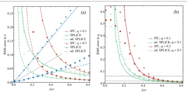
Figure5shows the resulting rms errors when estimatingδ, and q, by either IPC, SPLICE, or adapted SPLICE for the same cases of q as above. Here, we plot the results of Monte Carlo simulations for the three methods, overlaid with the relevant CRBs(except in the case of SPLICE (blue) where we instead overlay the numerically found rms error). First, we see in figure5(a) that the error when estimating δ diverges at low separations when
using either IPC or adapted SPLICE. This was to be expected since it is now known that the quantum CRB for estimatingδ between unequal intensity emitters diverges at low δ [20,21]. However, we also see that the
unadapted SPLICE measurement, which assumes equal intensity emitters, does surprisingly well in comparison. The rms error does not diverge at low separation. As seen in the previous section, for values of q above some critical value, i.e. qc=1/5, one can achieve rms errors lower than a given error threshold down to very low
separations. This is surprising given that the unbiased quantum CRB diverges at low separations. However, the SPLICE estimator,dˆSPL( )k = 8ps2k N, differs from the estimator in equation(9) primarily by the factor of
s2/v2, which manifests as a bias. Then for low skews, which occur for q≈1/2 or as δ→0, the unadapted
Figure 3.(a) Lowest δ that can be distinguished from 0 by 5 standard deviations (rms error δ / 5) using unadapted SPLICE (solid blue), or IPC (dashed red). Lowest resolvable δ scales as N−1/2for SPLICE but as N−1/4for IPC. Inset: Monte Carlo simulations showing the rms error in dˆ whenδ=0.2σ. Semi-transparent lines show the Cramér–Rao bounds for each method. Dotted black line marksδ/5. (b) With equal intensities, but an unknown mean, first detect M photons with IPC to estimate the mean and align the SPLICE apparatus. Shown is the lowestδ estimated with rms error δ /5 for various fractions M/N. (c) Rms error in δ for SPLICE when emitters have unequal intensities(q and 1 − q). Here, δ=0.2σ and M=N/2. Dotted black line marks an rms error of δ/5. (d) Lowest separation estimated with SPLICE and IPC for unequal intensity emitters. For q<0.2 SPLICE cannot achieve an rms error ofδ/5 for any δ. For 0.2<q<0.5, or a larger rms error threshold (dotted lines), the lowest resolvable δ scales as N−1/2for SPLICE and N−1/4for IPC.
SPLICE estimator can still achieve a low bias while retaining excellent scaling with N. The rms is ultimately lower bounded by2s M, the bias caused by misestimation of the mean. Once q<qc, the error threshold cannot be
reached for any separation even though the rms error decreases linearly withδ. Therefore, for scenarios with large skew, q<qc, we turn to the adapted SPLICE measurement. Infigure5(a), we see that the rms error
Figure 4. Monte Carlo results forN=106input photons and 1000 Monte Carlo repetitions. Root mean squared(rms) error of skew estimates for q=0.1 (circles) and q=0.3 (squares) as a function of separation. In the adapted SPLICE scheme (green, hollow) N/3 photons are used in the skew measurement, split evenly between the two projections. For IPC(red, solid) all N photons can be used for the skew estimate. Lines show the CRB for q=0.1 (solid) and q=0.3 (dashed) cases. As δ/σ decreases, the RMS error in skew given by adapted SPLICE dips well below the constant error given by IPC.
Figure 5. Monte Carlo results for N=106photons and 1000 Monte Carlo repetitions. Rms error of(a) δ, and (b) q estimates as a function of separation when q=0.1 (squares) and q=0.3 (circles) for IPC (solid red), SPLICE (solid blue) and adapted SPLICE (hollow green). Solid (q=0.1) and dashed (q=0.3) lines show the CRB for IPC and adapted SPLICE (see appendixC). (a) For
SPLICE, solid and dashed lines are numerically calculated rms errors(see appendixB), linear in δ for N2ps d2 2q(1-q). As
δ→0 the SPLICE rms error is2s M. Dotted black line marks an rms error ofδ/5. While the error for adapted SPLICE diverges (whereas it does not for SPLICE), there are values of δ (for q=0.1) where SPLICE cannot achieve an rms error below δ/5, but where adapted SPLICE can.(b) Since SPLICE does not provide an estimate of q, we only compare IPC and adapted SPLICE. Monte Carlo results that fall below the CRB lines imply biased measurements. Adapted SPLICE can achieve rms errors below thresholds of q/5 (dotted and dotted–dashed black lines) for smaller separations than IPC can.
diverges at low separations. This can be explained by the fact that when adapting the measurement to estimate bothδ and q, there are now different physical scenarios that can lead to a low skew: two near-equal intensity sources close together(q≈1/2, δ→0), or very disparate intensity sources far apart (q→0, δ?0). This was avoided in the unadapted SPLICE measurement by always assuming that q=1/2. Though the rms error for
aSPL
dˆ diverges for lowδ, there is still a range of δ which can be estimated below the error threshold even at low q. Additionally, the adapted SPLICE measurements allow one to make an estimate of q itself, which we show in figure5(b). We see that the error in qˆ also diverges at low δ. However, the adapted SPLICE measurement can
make estimates of q below a chosen error threshold, e.g. q/5, for lower separations than can be achieved by using IPC alone.
Finally for this section, we investigate a scenario where one emitter is much brighter than the other. Figure6
compares the adapted SPLICE scheme to IPC for estimatingδ when q ranges from 10−1to 10−4. Infigure6(a),
Monte Carlo simulations of adapted SPLICE(when δ=0.2σ) show relatively constant rms errors until
N~2ps2 q(1-q)d2, after which we see behavior close to the CRB, with the rms error scaling like1 N.
Using adapted SPLICE, if q is reduced by an order of magnitude, achieving afixed rms error threshold requires an order of magnitude more photons. Looking at the CRB for IPC infigure6(a), a drop in q by an order of
magnitude requires an additional two orders of magnitude of photons to achieve the same rms error threshold. This is due to the fact that the IPC estimator is biased until N
q q 2 1 4 4 2 2 ~ s
d ( - ) , below which the standard deviation
only scales like N−1/4. Monte Carlo simulations for IPC were computationally intensive and were not performed for input photon numbers of N>107
, though we found good agreement between simulations and the CRB for q=0.1 when N=106(see figure
5(a)).
We compare the CRB of IPC to that of adapted SPLICE infigure6(b), where we once again plot the smallest
resolvable separation below an rms error threshold ofδ/5. Note that since the biases of both the adapted SPLICE and IPC estimators are large for few photons, the error threshold will only be reached when the bias is low and rms error is dominated by the CRB. Crucially, we see that the slopes of these lines are quite different: the lowest resolvableδ using adapted SPLICE scales approximately as N−1/4, whereas using IPC it scales approximately as N−1/6. Furthermore, we see again that the required N for a givenδ scales linearly with q for adapted SPLICE, but quadratically with q for IPC. This is primarily determined by the amount of photons required for each scheme to overcome their low-N biases, which are given above. The adapted SPLICE scheme shows promising scaling advantages in photon number over IPC for emitters of very different brightness and separations below the Rayleigh limit.
5. Estimating higher moments
So far we have focused on a particular scenario with two emitters. In this section we discuss how the SPLICE scheme can be adapted to estimate higher moments of a source distribution, enabling the characterization of
Figure 6.(a) The rms error in estimating δ, using the adapted SPLICE (green) or IPC (red), when the actual separation is δ=0.2σ and one of the emitters is much brighter than the other(fraction given by q). Points show results from Monte Carlo simulations of the adapted SPLICE, allocating photon numbers equally between the mean(IPC), variance and skew measurements. Lines mark Cramér– Rao bound for adapted SPLICE and IPC for each value of q(see appendixC). The black dotted line shows where the rms error is equal
toδ/5. (b) Separations that can be estimated to within an rms error of δ/5 with N photons using adapted SPLICE (green) or IPC (red). Lines are calculated from the Cramér–Rao bounds in (a).
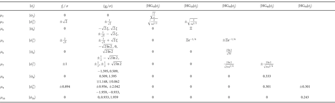
Table 1. Overlaps of SPLICE projectors∣f ñj with HG modes. Overlaps higher than the leading order HG modes are not shown but can be straightforwardly solved. The positions of the single-modefiber are given by fj, and the positions of
the glass edges{gj} in units of σ. The positions for moments 8 and higher were solved numerically.x =erf-1(1 2), 2 2 e
2 x X = - p -x. j f ñ ∣ fj/ σ {gj/σ} áHG10∣fjñ áHG20∣fjñ áHG30∣fjñ áHG40∣fjñ áHG50∣fjñ μ2 ∣f ñ2 0 0 2 p μ3 f ñ3 ∣ 2 1 2 2 e1 2 p 2 e1 2 p 4 m ∣f ñ4 0 - 2 ,x 2x 0 Ξ 2 1 3 x - , 5 m ∣f ñ5 2 3 1 2 3 x + 0 Xe-1 6 Xe-1 6 2 ln 2 , 0 - , 6 m ∣f ñ6 0 2 ln 2 0 0 2 ln 2 3p 2 ln 2 1 2 - , 7 m ∣f ñ7 ±1 1 2 , 1 2 ln 2 2 + 0 0 2 ln 2 3 ep1 4 2 ln 2 3 e1 4 p −1.595, 0.509, 8 m ∣f ñ8 0 0.509, 1.595 0 0 0 0.333 m1.148, m0.062 9 m ∣f ñ9 ±0.894 0.956,2.042 0 0 0 0.301 ±0.301 −1.959, −0.933, 10 m ∣f ñ10 0 0, 0.933, 1.959 0 0 0 0 0.243 9 New J. Phys. 21 (2019 ) 093010 K A G Bonsma-Fisher et al
more complex shapes. Here we take a more general distribution of point sources along the x-axis by considering the density matrix of an incoming photon as
XF X x y x X y x y d , d d , , , 12 X X X
ò
r y y y y = = --¥ +¥∬
( )∣ ⟩⟨ ∣ ∣ ⟩ ( )∣ ⟩ ( )where we take the spatial extent of F(X) to be less than the width of the PSF (σ), firmly in the sub-Rayleigh regime. SPLICE measurement configurations are found using a similar method as in section4: usingπ phase-shifts and a single-modefiber, each translatable along the x-axis, zero overlap with all lower HG modes can be obtained. We write a generalized SPLICE mode as
x y x y x y x y x g 1 2 d d , , , e sgn , 13 j j j x f y i n j i 2 4 1 , j2 2 j 2
f ps f f = = s --¥ +¥ - - + =∬
∣ ⟩ ( )∣ ⟩∣ ⟩ ( ) ( ) ( ) ( )where fjis the corresponding position of the single-modefiber, and the set {gj} represent the positions of the
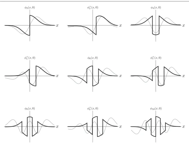
right-most edges of njπ phase-shifters, so that for every x<gjthere is a phase shift ofπ. Figure7plots the
SPLICE functionsfj(x, 0) for modes up to j=10. Likewise, table1details thefiber positions fj, phase-shifter
positions{gj}, and overlaps with HG modes up to j=10. Projective measurements onto the mode∣f ñj succeed
with probability
pj =Tr r f fj j =
ò
dXF X f yj X 2. 14-¥ +¥
( ∣ ⟩⟨ ∣) ( )∣⟨ ∣ ⟩∣ ( )
By casting the SPLICE modes into the HG basis, we can use the same treatment as in[22] to show how thejth
statistical moment of F(X) is extracted in the sub-Rayleigh regime. Here we will consider when the SPLICE measurements are centered aboutμ1, the mean of F(X), which is to say that the specified positions of the fiber
Figure 7. Generalized SPLICE functionsfj(x, 0) (solid black, equation (5)) are used to estimate the jth moment. The relevant HG
functions(gray, equation (7)) are plotted for comparison: HGk,0(x, 0) for the k2 thmoment; and(HGk,0(x, 0)+HGk+1,0(x, 0)) 2 for the2k+1thmoment(see [22]). For odd j only the plus superpositions are shown for brevity; the minus superpositions are
and phase-shifters in table1should be made relative toμ1. As in the previous section, intensity measurements
can be used to efficiently estimate the mean.
Table2shows the probability of success for a projective measurement onto the SPLICE mode∣f ñj. The results show leading order terms in a series expansion ofD =(X-m1) s, the distance from the point source at X to the mean of F(X). It can be seen from table2that∣áf yj∣ Xñ µ D∣2 j(for odd j this is true once the difference∣áf y+j∣ Xñ -∣2
j X
2
f y
á - ñ
∣ ∣ ∣ is taken). This directly implies that the integral in pjgives the expectation value of X( -m1)j, which is the
jth moment of F(X) centered on the mean. This is true for any choice of F(X) in the sub-diffraction regime. The distribution F(X) is uniquely determined by its moments. Measuring up to the 10th moment one can, in principle, completely characterize distributions with 10 or fewer degrees of freedom, e.g. 5 sources with unequal intensities. Though the SPLICE scheme is capable of estimating arbitrary moments of F(X), we note here that higher moments require substantial precision in the placement of the phase-shifters. For example, the∣f ñ10 projection shows competitive contributions from lower orders ofΔ/σ if the values of {g10} differ from ideal by more than 10−3σ. One
could imagine achieving this level of precision for space telescopes which have PSF on the meter-scale.
6. Conclusions
The SPLICE measurement scheme, initially envisioned to demonstrate super-resolution in a highly idealized scenario, can also be advantageous in a more realistic system, such as where the point sources have unequal intensities. Surprisingly, the SPLICE measurement, without any modification, outperforms IPC for resolving lower separations at moderately disparate intensities. Eventually, the skew of the source distribution becomes so substantial that the SPLICE measurement retains a large bias. But in this case a simple adaptation to SPLICE regains an advantage in resolving small separations over IPC. We found, by comparing Cramér-Rao bounds, that the advantage over IPC persists to very imbalanced intensities(at least q=10−4), lending some credence to the use of novel sub-Rayleigh imaging techniques for exoplanet detection(Earth is 1010times fainter than the Sun at visible wavelengths[23]). The adapted SPLICE scheme can be realized without increasing the complexity
of the scheme: the only requirements remain aπ phase-shift about an edge and a single-mode fiber, now translatable along the transverse axis. Thus, we imagine that an experimental demonstration of sub-Rayleigh imaging for emitters of very different brightness can be performed in much the same style as[12]. This work uses
a Gaussian-shaped PSF. However, for any even PSF we expect a SPLICE-like measurement can be constructed by following our treatment of setting the phase andfiber parameters to minimize overlap with lower basis states for a variance measurement and, additionally, matching overlaps between adjacent basis states for a skew
measurement. We have focused on a source distribution in one dimension, however, it is a straightforward extension to also include measurement along the y-axis to investigate two-dimensional distributions. Finally, we have proposed extensions to the SPLICE scheme beyond measurements of the variance and skew, up to the 10th statistical moment. These measurements add some complexity to the scheme, requiring multiple edges between regions ofπ and zero phase-shifts. We imagine that this could be performed with a spatial light modulator followed by an array of single-modefibers. The ability to measure higher statistical moments of a source distribution enables one to reconstruct spatial structure.
Table 2. Squared overlaps of SPLICE projectors∣f ñj with∣y ñX , an
emitter at position X convolved with the point spread function. SPLICE measurements are centered onμ, the mean of F(X). Results are expanded to leading order inD =(X-m s) .x =erf-1(1 2).
j f ñ ∣ ∣áf yj∣ Xñ∣2 2 f ñ ∣ 1 2 2 4 D + D p ( ) 3 f ñ ∣ e 1 2 2 1 2 3 1 12 4 5 D D - D + D p
(
)
( ) 4 f ñ ∣ 1 e 4 2 22 4 6 x -xD + (D) 5 f ñ ∣ e 4e 4 1 3 5 5 2 24 6 7 2 2 2 1 3 2 D D - D + D x p x -x-(
( ))
( ) 6 f ñ ∣ ln 2 288 6 8 2 D + D p ( ) ( ) 7 f ñ ∣ ln2 288e 6 1 2 7 11 2ln2 40 8 9 2 1 4p D D - D +D-(
)
( ) ( ) ( ) 8 f ñ ∣ (1.80´10-5)D +8 (D10) 9 f ñ ∣ (1.48´10-5)D 8 (6.61´10-6)D9 3.99 10 6 10 11 -( ´ -)D + (D ) 10 f ñ ∣ 4.60 10 7 10 12 10 ´ + D s - D ( ) ( )Acknowledgments
The authors would like to thank Mankei Tsang, John Donohue, Noah Lupu-Gladstein and Arthur Ou Teen Pang for fruitful discussions. This work was supported by Natural Sciences and Engineering Research Council (NSERC) of Canada and the Canadian Institute for Advanced Research (CIFAR).
Appendix A. Monte Carlo simulations
Monte Carlo simulations of SPLICE, adapted SPLICE, and IPC were performed using Wolfram Mathematica 11. For all simulations the PSF width is set asσ=1. First, we describe the IPC simulations. The inputs are the actual values ofδ, q and c as well as the number of incident photons N. We then draw N position values xifrom the
intensity distribution x q 1 q 2 e 1 1 2 e . A.1 2 2 x c 2 2 x c 2 2 2 2 2 2 ps ps = - d + - -s d s - + -( ) ( ( )) ( ) ( ( )) ( )
Note that we take the center of the distribution to be c=0 throughout the simulations, since the SPLICE measurement is independent of c when aligned about the mean of( ). Next, we estimate the mean, variancex
(subtracting σ2), and skew of the resulting set of position values {x}
x N x 1 , A.2 i i
å
= ¯ ( ) v N x x 1 1 i i , A.3 2 2å
s = - - -ˆ ( ¯) ( ) s N N 1 N 2 i xi x . A.4 3å
= - - -ˆ ( )( ) ( ¯) ( )The estimatesdˆand qˆ are then calculated using equations(9) and (10). Importantly, we rejected Monte Carlo
trials wherevˆ<0since it led to unphysical estimates ofδ. This is a substantial cause of the bias in the IPC measurement at low N. We note that other methods, such as regression, for estimatingδ using IPC were explored but did not perform better than inverting the variance and skew as above.
Next, we outline how the Monte Carlo simulations for SPLICE, and adapted SPLICE, were performed. For the variance measurement the probability of a photon detection, as a function ofδ, q, c and the position of the fiber and phase-shifter edge ( f and g, respectively), is
P q f g c q f g c e erf 2 2 2 2 1 e erf 2 2 2 2 . A.5 2 2 f c f c 2 2 8 2 2 2 8 2 d s d s = - + + + - - + -d s d s - + -⎡ ⎣ ⎢ ⎛⎝⎜ ⎞ ⎠ ⎟⎤ ⎦ ⎥ ⎡ ⎣ ⎢ ⎛⎝⎜ ⎞ ⎠ ⎟⎤ ⎦ ⎥ ( ) ( ) ( )) ( ))
Notice that when aligned at the mean, f= =g m1= -c (1-2q)d 2, that c drops out entirely. To estimate the variance, given an average of N incident photons, we draw a number k from a Poisson distribution with λ=N×P. The variance is then estimated as v 2 k
N
2 1 2
1
ps
=
(
++)
ˆ . The factors of 1/2 and 1 are added to the numerator and denominator so that the variance is never estimated to be 0. For thefirst-generation SPLICE scheme the separation is estimated as 4 ˆ . When the mean of the distribution is not known a priori, M photonsv
are detected with IPC to estimate it, and so the values of f and g are set equal to x¯.
For the adapted SPLICE scheme we add two measurements to estimate the skew. The probabilities of photon detection,p3+andp3-, remain the same as equation(A.5), where the fiber and phase-shifter edge are moved to
f= +x¯ 2 s, g= +x¯ s 2for thefirst measurement, and f= -x¯ 2 s, g= -x¯ s 2for the second. Incident photons(N), are evenly divided between these two measurements, and we draw two numbers,k+and k-,
from Poisson distributions with meansl = N 2´p3. The skew estimate is calculated as sˆ= 2eps3
(
kN+-k2-)
.We typically allocate incident photons evenly between the measurements such that N/3 are used to estimate the mean with IPC, N/3 are used to estimate the variance, and N/6 are used in each of the skew measurements.
Appendix B. Expectation value of SPLICE estimator in certain limits
The number of photon detections(k) using the SPLICE measurement (∣f ñ2), for a fixed number of input
photons(N), is drawn from a binomial distribution with probability p2 = áf r f2∣ ∣ 2ñ. However, since we take N to be a Poissonian average number of incident photons, k is then drawn from a Poisson distribution with mean
N p2 N
8 2
2
l = ´ » psd in the simplest case. Since the probability of detection depends onδ2to leading order, the estimator for the separation(dˆSPL) depends on k, specificallydˆSPL( )k = 8ps2k N. We are then interested in
the expectation value E k k k k
e k
= å -ll [ ]
! in the low, and high, limits of N. Forl =N´p2 , the1 first few
terms in the sum give a good approximation to the expectation value, and we have
E k 1 2 ... 2 ... 1 1 2 . B.1 2 2 2 l l l l l l = - + - + + » - -⎛ ⎝ ⎜ ⎞ ⎠ ⎟⎛ ⎝ ⎜ ⎞ ⎠ ⎟ ⎛ ⎝ ⎜ ⎞⎠⎟ [ ] ( ) The bias is» l( l -1), and, since E k[ ] =l, the variance is V[ k]»l. Notably, this implies that for low N, the variance of the SPLICE estimator is constant: V[ˆdSPL]=d2. This behavior continues untilλ∼1. We
consider N to be large whenl =N´p2 . In this case we can expand the estimator around its mean value1
k k k E k 1 2 1 8 ... 1 8 . B.2 3 2 2 l l l l l l l = + - - - + » -( ) ( ) [ ] ( )
The bias of the SPLICE estimator in this case is
N p s
d , and the variance is V SPL N
2 2
d = ps
[ˆ ] .
When the mean of the position is not known a priori, so that the SPLICE measurement may be misaligned, the probability of a photon detection picks up an extra term which must be taken into account when calculating the expectation value of the SPLICE estimator. Similarly, when the equal-intensity assumption is relaxed the probability of detection is modified, becoming
Nq 1 q N q q q N q q 2 2 1 1 2 3 2 1 2 1 . B.3 2 2 3 4 2 2 2 2 l m d ps m d ps m ps d s D » - + D - - + D ⎛ - -⎝ ⎜ ⎞ ⎠ ⎟ ( ) ( ) ( )( ) ( ) ( )
The misalignmentΔμ is a random normal variable with mean 0, and variance σ2/M, where M is the number of photons used for estimating the mean with a round of IPC. To calculate the expectation valueE[ˆdSPL]we must
integrate over the probability density ofΔμ as well as take the Poissonian sum. In the main text, we only do this for the large N case
E N M 8 1 8 e 2 d , B.4 SPL 2 2 M 2 2 2
ò
d ps l m l m ps m = D -D D -¥ ¥ - m s D ⎛ ⎝ ⎜⎜ ⎞ ⎠ ⎟⎟ [ ˆ ] ( ) ( ) ( ) ( )which we integrate numerically. For large N, and subsequently large M, E[ˆdSPL]µdand E SPL
2 2
d µd
[ˆ ] .
Appendix C. CRB for adapted SPLICE and IPC
The CRB for a parameter estimate is calculated by inverting the Fisher information matrix. The Fisher information matrixa, given P, the probability of getting a certain result a, and the parametersδ, q, and c is
P 1 . C.1 a P P P q P P c P P q P q P q P c P P c P q P c P c 2 2 2 = d d d d d ¶ ¶ ¶ ¶ ¶ ¶ ¶ ¶ ¶ ¶ ¶ ¶ ¶ ¶ ¶ ¶ ¶ ¶ ¶ ¶ ¶ ¶ ¶ ¶ ¶ ¶ ¶ ¶ ¶ ¶ ⎛ ⎝ ⎜ ⎜ ⎜ ⎜ ⎜⎜ ⎞ ⎠ ⎟ ⎟ ⎟ ⎟ ⎟⎟
( )
( )
( )
( )For IPC, P= ( ), the intensity distribution. The full Fisher information matrix x is then integrated over all measurement outcomes=
ò
-¥xdx¥
. The resulting matrix is then inverted with thefirst entry corresponding to the CRB for estimatingδ. To leading order in δ the IPC CRB is q
Nq q 6 1 2 1 2 6 2 2 4 s d -( ) ( ) . For SPLICE, P 1p 2 2
= for the variance measurements, and P 1p , p
4 3 1 4 3
= + -for the skew measurement. The
factors of 1/2 and 1/4 represent the fact that photons are allocated evenly between the variance and skew measurements. We assume that the mean is known(Δμ=0) and so do not include the round of IPC for mean estimation here. We account for this by scaling the photon number N by a factor of 2/3 to account for 1/3 of incoming light being allocated to IPC for the mean estimate. We use a 2×2 Fisher information matrix in this case, leaving out c. The Fisher information matrix is then= 12p2+ 211-p2+ 41p3 + 411-p3 + 41p3 + 411-p3
+ + - -.
To leading order inδ, the adapted SPLICE CRB is e q
N q q 8 1 2 2 3 1 2 4 2 p s d -( )
( ) ( ) . The adapted SPLICE and IPC CRBs are shown in
figures4–6in the main text.
ORCID iDs
Kent A G Bonsma-Fisher https://orcid.org/0000-0002-5581-8892
References
[1] Rayleigh F R S 1879 Phil. Mag. 58 261–74
[2] Tsang M, Nair R and Lu X M 2016 Phys. Rev. X6 1–17
[3] Lupo C and Pirandola S 2016 Phys. Rev. Lett.117 1–5
[4] Nair R and Tsang M 2016 Opt. Express24 3684
[5] Nair R and Tsang M 2016 Phys. Rev. Lett.117 1–5
[6] Řeháček J, Paúr M, Stoklasa B, Hradil Z and Sánchez-Soto L L 2017 Opt. Lett.42 231
[7] Tsang M 2018 J. Mod. Opt.65 1385–91
[8] Lu X M, Krovi H, Nair R, Guha S and Shapiro J H 2018 Npj Quantum Inf.4 64
[9] Paúr M, Stoklasa B, Hradil Z, Sánchez-Soto L L and Řeháček J 2016 Optica3 1144
[10] Yang F, Tashchilina A, Moiseev E S, Simon C and Lvovsky A I 2016 Optica3 1148
[11] Tang Z S, Durak K and Tsang M 2016 Opt. Express24 22004–12
[12] Tham W K, Ferretti H and Steinberg A M 2017 Phys. Rev. Lett.118 070801
[13] Donohue J M, Ansari V, Řeháček J, Hradil Z, Stoklasa B, Paúr M, Sánchez-Soto L L and Silberhorn C 2018 Phys. Rev. Lett.121 090501
[14] Napoli C, Piano S, Leach R, Adesso G and Tufarelli T 2019 Phys. Rev. Lett.122 140505
[15] Ang S Z, Nair R and Tsang M 2017 Phys. Rev. A95 063847
[16] Yu Z and Prasad S 2018 Phys. Rev. Lett.121 180504
[17] Parniak M, Borówka S, Boroszko K, Wasilewski W, Banaszek K and Demkowicz-Dobrzański R 2018 Phys. Rev. Lett.121 250503
[18] Tsang M 2019 Phys. Rev. A99 012305
[19] Zhou S and Jiang L 2019 Phys. Rev. A99 013808
[20] Řeháček J, Hradil Z, Stoklasa B, Paúr M, Grover J, Krzic A and Sánchez-Soto L L 2017 Phys. Rev. A96 062107
[21] Řeháček J, Hradil Z, Koutný D, Grover J, Krzic A and Sánchez-Soto L L 2018 Phys. Rev. A98 012103
[22] Tsang M 2017 New J. Phys.19 023054