An analysis of surface area estimates of binary volumes under three tilings

An Analysis of Surface Area Estimates of Binary

Volumes Under Three Tilings

by

Erik G. Miller

Submitted to the Department of Electrical Engineering and

Computer Science

in partial fulfillment of the requirements for the degree of

Master of Science in Electrical Engineering

at the

MASSACHUSETTS INSTITUTE OF TECHNOLOGY

June 1997

@

Massachusetts Institute of Technology 1997. All rights reserved.

Author ...

Department of Electrical Engineering and Computer Science

May 18, 1997

Certified by ...

Iertho'dK. P. Horn

Professor of Electrical Engineering and Computer Science

Thesis Supervisor

Accepted by ...

..--.

..

...

Arthur C. Smith

Chairman, Departmental Committee on Graduate Students

An Analysis of Surface Area Estimates of Binary Volumes

Under Three Tilings

by

Erik G. Miller

Submitted to the Department of Electrical Engineering and Computer Science on May 18, 1997, in partial fulfillment of the

requirements for the degree of Master of Science in Electrical Engineering

Abstract

In this paper, we first review local counting methods for perimeter estimation of piecewise smooth binary figures on square and hexagonal grids. We verify that better perimeter estimates can be obtained on a hexagonal grid. We then compare surface area estimates using local counting techniques for binary three-dimensional volumes under three distinct tilings: the cubic, truncated octahedral, and rhombic dodeca-hedral tilings. It is shown that under certain assumptions of piecewise smoothness, the mean error of surface area estimates is smaller for the truncated octahedral and rhombic dodecahedral tilings than for the standard cubic or rectangular prism tilings of space. Additional properties of these tessellations are reviewed and potential ap-plications of better surface area estimates are discussed.

Thesis Supervisor: Berthold K. P. Horn

Acknowledgments

It was an honor and a pleasure to work with Professor Berthold K. P. Horn on this project. His enthusiasm and support for the "basic research" presented here was a great motivating force. I was most grateful for his willingness to discuss the abstruse and obscure details of this project at a moment's notice.

I thank in particular Chris Stauffer for several "breakthrough" discussions and ideas about 3-D geometry, without which I may not have been able to turn this work into a thesis. I have a debt to Oded Maron and to Carl de Marcken for actually reading an entire draft and making helpful suggestions.

I also thank Polina Golland, Jeremy De Bonet, and Greg Galperin for helpful discussions related to this work.

I would like to thank Professor Paul Viola for his support during this project and for his patience in my completion of it. Professor Eric Grimson has also been pivotal in providing a supportive and relaxed atmosphere during my first two years at MIT.

Contents

1 Introduction

1.1 Some Definitions ...

1.2 Local Counting Algorithms . . . . 1.2.1 Exact Euler Number Computation . . . 1.2.2 Arbitrarily Accurate Area Computation 1.2.3 Accurate Perimeter Computation? . . . 1.3 Organization of the Thesis . . . . 2 Two Dimensional Tilings

2.1 Choice of Tilings ...

2.2 The Cartesian Square Tiling . . . . 2.3 Hexagonal Tilings ...

2.4 Length Bias vs. Centered Length Bias . . 2.5 Error Extrema and the Squared Centered 1

2.5.1 Error Extrema ...

2.5.2 Squared centered error . . . . 2.6 Summary of results for 2-D ...

3 Three Dimensional Tilings

3.1 Cubic Tilings ...

3.1.1 Mean Estimated Area . . . . 3.1.2 Area Bias, Centered Area Bias, and 3.1.3 Summary of Results for Cubic Grid

ias

S.ther Sta. . . .istics ..

Other Statistics. 10 10 11 12 14 14 20 21 . . . . 21 . . . . . 22 . . . . 23 . . . . . 26 . . . . . 28 . . . . 28 . . . . . 28 . . . . 30 31 32 34 37

3.1.4 Other Choices of Grids ... 3.2 The Truncated Octahedron ...

3.2.1 The Estimated Area Function for Truncated Octahedral Grids 3.2.2 Other Statistics on the TO Grid . . . . 3.3 The Rhombic Dodecahedron . . . ..

3.3.1 The Estimated Area Function for Rhombic Dodecahedral Grids 3.4 Summary of Results for 3-D ...

4 Discussion and Applications

4.1 M edical Applications ...

4.1.1 The Practicality of Using TO and RD Voxels . . . . 4.2 Industrial Applications ...

4.3 Other Properties of the RD and TO Tilings . . . . 4.3.1 Tessellation as Sampling . . . . 4.3.2 Topology: Thinning Algorithms and Finite Element Methods . 4.3.3 Geometry of Construction . . . . 4.4 Future W ork . . . ..

A Tilings

A .1 T ilings . . . . A.1.1 Dirichlet Domains and Dirichlet Tessellations . . . .

A.1.2 Non-Dirichlet Tessellations . . . .

B Some Identities

B.1 Regions of Symmetry ...

B.2 Alternative Parameterizations of Planar Segments . . . .

C Derivation of Closed Form Solutions to Mean Estimated Area Inte-grals

C.1 The Truncated Octahedron Grid . . . .

C.2 The Rhombic Dodecahedron Grid .... . . . .

52 53 53 54 54 54 55 58 58 58 60 61 61 62 64 64 66

D Tiling a Planar Patch: Some Additional Figures 69

D.1 The Truncated Octahedron Projections . ... 69

List of Figures

1-1 The tessellation of a circle on a square grid. . ... 11

1-2 Euler number on various grids... ... .. 13

1-3 The approximation of a boundary with a finite number of fixed-length line segments... ... 15

1-4 Estimating line length using city block distance. . ... 17

1-5 Pixel Size Comparison... ... 18

2-1 Bias symmetry regions for square and hexagonal tessellations ... 23

2-2 Lines on a Hexagonal Grid. ... 24

2-3 Hexagonal Grid Segments. ... 24

3-1 A planar patch and its associated angles. . ... 32

3-2 Symmetric Region of Integration for Cubes, TO's, and RD's... 33

3-3 Area error and centered area error for the cubic tiling. . ... 36

3-4 Truncated Octahedron ... 40

3-5 Truncated Octahedron Views. ... 41

3-6 Truncated Octahedron Surface. . ... .. 42

3-7 Visibility of Voxels in a TO Tiling. . . . . ... . 43

3-8 The rhombic dodecahedron. . ... .... 46

3-9 Projections of the rhombic dodecahedron. . ... 47

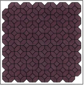
3-10 Surface tessellation with RD's shown from z-axis. . ... . . 48

3-11 Estimated area error and centered estimated area error as a function of surface angle for different tessellations. ... . . . . . 50

A sphere rendered with cubes ...

A sphere rendered with truncated octahedra. ... A sphere rendered with rhombic dodecahedra. .... Square and Triangular Tessellations . . . . .

An irregular Dirichlet Tessellation . . . . .

A shifted square tessellation of angle 0. ... 4-1 4-2 4-3 A-1 A-2 A-3 D-1 D-2 D-3 D-4 D-5 D-6 D-7 D-8 D-9 projections.

D-10 The oblique view of a planar patch along with its three major projections. 76

. . . . . 55

. . . . . 56

. . . . . 5 7

A planar patch represented with truncated octahedra . The projection of the planar patch onto the x-y plane. The projection of the planar patch onto the x-z plane. .. The projection of the planar patch onto the y-z plane.. The oblique view of a planar patch along with its three major A planar patch represented with rhombic dodecahedra. .

The projection of the planar patch onto the x-y plane. . The projection of the planar patch onto the x-z plane. .. The projection of the planar patch onto the y-z plane. ..

List of Tables

2.1 Some estimated length statistics of a random unit-length line segment process under square and hexagonal tessellations. Notice that while the square and hexagonal grids have equal length bias, the hexagonal grid has a lower centered length bias as well as a smaller range of possible values for length estimates of a unit-length line segment. ... . 30 3.1 _{Some statistics for random plane processes on tessellations of cubes,}

Chapter 1

Introduction

To represent images or volumes in a digital computer, they must be discretized. This discretization leads to errors in the computation of such fundamental properties of objects as perimeter, area, volume, and surface area. Not surprisingly, the magnitudes of these errors depend upon the particular discretization used. There are an infinite variety of discrete approximations for any planar figure, from the spatial frequency decompositions used in signal processing to parameterized NURB surfaces used in the CAD/CAM world. In this thesis, we focus on a particular class of discretizations: the tessellation of planar figures and solid volumes. Tessellations are approximate representations particularly convenient in computer vision and graphics.

1.1

Some Definitions

We define the tessellation of a figure (in either two or three dimensions) as the dis-cretization of the figure into a finite number of continuous regions, each having a constant value (See Figure 1-1). The value of each region is some measure of the original figure in that vicinity, such as a point sample of the figure at the centroid of the region or a spatial average over the region. In two dimensions, these regions are typically dubbed pixels, for picture elements, and in three dimensions voxels, for vol-ume elements. In this thesis, we use the term tiling synonymously with tessellation, and each element of a tessellation is sometimes referred to as a tile, especially if the

dimension is unspecified. The term grid shall be used to denote the specific arrange-ment of tiles used to cover a space. For example, squares can be placed in the common Cartesian grid (like ordinary graph paper), or can be arranged so that each row is offset by some distance from the previous row (as in a brick wall). When discussing a tiling by a particular tile which has more than one possible associated grid (only the square and cubic grids in this paper), it will be assumed unless stated otherwise that the Cartesian grid is intended. Tiling a figure on a Cartesian square or rectangular grid (such as that of a typical raster display) is frequently called rasterization [4].

'H

-K-!__rlZLYIPII _IPI

Figure 1-1: The tessellation of a circle on a square grid. Here, the original figure was sampled at the center of each tile, and this value was copied across the whole tile. The figure on the left is a continuous binary image. The figure on the right is a

discrete binary image.

In the following analyses, we restrict our focus to binary images and volumes, i.e. data sets in which each pixel or voxel has one of two values (black or white, 0 or 1, etc.). Much of the previous work on properties of tessellations does the same: [2, 6, 7, 9]. Prior to tessellation we call a binary image continuous. After tessellation, it becomes a discrete binary image. The same terminology applies to volumes.

1.2

Local Counting Algorithms

Much of the work in discrete binary image processing has focused on local counting

algorithms [7, 11]. These techniques involve computing functions of figures when only

local image information is available for computations, and local results are reported to a global accumulator. For example, in a black and white image, the perimeter of a tessellated figure can be computed using a local counting scheme as follows: a

processor at each black pixel reports to the global accumulator the length of its border with neighboring white pixels. The sum of the results from each processor is the exact perimeter of the tessellated figure. It is also a perimeter estimate (not always a good one!) of the originally imaged object from which the tessellated figure was derived. Local counting algorithms have been motivated in part by their inherent parallelism and simplicity of implementation, making them ideal for use on fine grain, highly parallel computers.

In two dimensions, there are three common functions which can be computed using local counting schemes: area, perimeter, and Euler number (a topological measure equal to the number of objects in an image less the number of holes). All of these functions obey the additive set property [9], the condition which allows the individual local measures to be combined into a global measure. Local counting algorithms produce exact results for these three functions on tessellated figures. However, if we use the value of a function computed for a tessellated figure as an estimate of the value of that function for the figure from which it came, we may get significant errors. And as we shall see, the error behavior of these algorithms varies significantly under different tessellations. We shall also see that while increasing the resolution of our grid can give us arbitrarily good measures of both Euler number and area, this is not the case for perimeter measures.

1.2.1

Exact Euler Number Computation

A figure's Euler number is by definition an integer, and it can be computed exactly even after a figure has been discretized provided that the discretization of the figure did not alter its topology in any way. If we make the tessellation too coarse, we will begin to lose information about the figure's topology. While for certain figures, one may be able to maintain the correct Euler number using a coarser hexagonal tessellation than with a similar resolution square tessellation, we can be sure that we can perfectly represent Euler number with some finite sized tessellation for either grid. That is, for all smooth figures f with well defined Euler numbers,

3n < oo : E'. (f) = E (f), (1.1) where E is the original figure's Euler number and En is the estimate of E on a grid with n pixels of a particular shape.

In Figure 1-2, we are unable to represent the Euler number of a continuous "V-shaped" region unambiguously with a coarse square tessellation (A). This is not an adequate representation since it is not clear whether we have one or three "holes" in the middle of the figure. A finer square tessellation (B), however, does the job. Here, we can unambiguously determine the true topology of the original figure. In (C), we were able to achieve this same result with a coarse hexagonal grid, although it is not true in general that a hexagonal grid will be able to represent exact Euler number with fewer pixels.'

The main point, however, as summarized in Equation 1.1 is that we can always compute Euler number exactly by choosing a small enough grid, regardless of the

shape of the pixels we use. This condition does not hold for other measures computed

with local counting schemes.

B C

Figure 1-2: Euler number on various grids. A. Here, it is not clear whether the figure has one, two, or three holes. B. Increasing the resolution enough will always solve the problem. C. Sometimes, but not always, the hexagonal grid provides a more efficient representation of a figure while preserving the original Euler number.

1Horn [9] points out that Euler number on a hexagonal grid is never ambiguous since there is no ambiguity in the definition of adjacency. The Euler number on a square grid can be ambiguous since

it is not clear whether two pixels touching by a corner are adjacent [2, 6]. However, this does not in general mean that we can represent the true topology of a figure more efficiently on a hexagonal

grid. The verity of this conjecture is not addressed here.

_ · _ _ _ _

1.2.2

Arbitrarily Accurate Area Computation

In particular, we cannot recover the exact area of a figure after it has been tessellated. It is not hard to see that for common figures with piecewise smooth borders, that the expected magnitude of the relative error in the computation of area is related to the ratio of the number of pixels which intersect the figure's border to the number of pixels completely contained within the figure. For plane figures whose borders are piecewise smooth and continuous, this ratio approaches zero as the area of each pixel goes to zero. That is:

lim A' (f) = A(f), (1.2) where f is again a piecewise smooth figure, n is the number of pixels used to represent the figure, and A' (f) is the approximate area based on a local counting algorithm for area computation, and A (f) is the true area of the figure. This result holds for all convex tessellations. While different tessellations may give better results for a certain number of pixels, we can obtain an error as small as we like by choosing small enough pixels, regardless of the shape of the pixels.

1.2.3

Accurate Perimeter Computation?

While Euler number and area can be approximated with arbitrary accuracy by merely increasing the resolution of our grid, the estimation of perimeter presents a special problem. Before embarking on an analysis of perimeter, however, we make the fol-lowing simplification.

Random Line Segment Length Estimation as a Substitute for Random Plane Figure Perimeter Estimation

We want to show, in an informal way, that certain statistics of random figure processes will have the same value as the equivalent statistics for random line processes. If we can do this, we have simplified our analysis of perimeter estimate to one of line segment length estimates. This will depend upon restricting the class of figures we are analyzing as well as making certain assumptions about the meaning of "random".

We note that each member of the set of simple, closed, piecewise smooth, planar curves can be "closely" approximated by a finite number of constant length line segments. Figure 1-3 illustrates this idea. If we choose a large enough number of

., ` t'-" - i---t-'-- .• i • , i -I , : I 7

', ,

i-V-

-:...

_

; -

-Figure 1-3: The approximation of a boundary with a finite number of fixed-length line segments. By representing a boundary as piecewise linear, we greatly simplify the analysis of the boundary's behavior under various tessellations.

segments with which to approximate a curve, then each segment of the curve will be arbitrarily well approximated by a line segment. The perimeter of this approximation can be made arbitrarily close to the true perimeter of the figure, which is achieved in the limit when the length of each segment goes to zero and the number of segments goes to infinity. Such a construction follows the reasoning in the derivation of the integral of arc length along the curve.

Now we are interested in the estimation of perimeter for "arbitrary" or "random" planar figures, since we wish to examine the expected values of various functions of estimated perimeter for any figure we may encounter. We choose to define

ran-dom piecewise smooth planar curves so that figures of any orientation and position

are equally probable. That is, we define random so that if a figure F has probabil-ity densprobabil-ity P, then an arbitrary rotation and translation of that figure F' also has probability density P. For the purposes of this paper, we do not need to further restrict our notion of random, since we are only interested in showing that border segments of any orientation are equally probably. For example, it is of no concern to us whether a large piecewise smooth planar figure is more or less probable than a smaller piecewise smooth planar figure, since approximations to both (over all of their possible orientations) will contribute equally to the uniform distribution of line segment orientations in our analysis. To use the terminology of stochastic geometry, we are restricting our density of random piecewise smooth simple closed curves to

be invariant to the choice of coordinate system, a common approach when discussing geometric stochastic processes [23].

If curves of any rotation are equally probable then we can choose finite line segment approximations to those curves in such a way that the orientation of the line segments (relative to the x-axis) is also evenly distributed. That is, we are interpreting "random figures" to be well approximated by collections of "random line segments". Hence, the perimeter of these random curves can be estimated in the same way as the length of random line segments. In this way, we reduce the problem of the analysis of random curves to the analysis of random line segments, a considerable simplification.

City Block Distance

We now address the problem of estimating the length of a line segment (and hence a piecewise smooth curve) on a finite grid. Figure 1-4 shows the basic approach to estimating the length of a line segment using the so called city block distance [15]. This figure represents the worst case scenario in which we overestimate the length of the line by a factor of V2 % 1.414. We again ask the question of whether increasing the resolution of the grid will improve the estimate. The answer is that up to a certain point, increasing the resolution will improve perimeter estimates, but that beyond a certain resolution, we will not be able to significantly reduce the perimeter error by increasing the resolution.

Below, we examine the reasons for this statement. Consider a polygon represented on two grids of differing resolution, as in Figures 1-5A and 1-5B.

Case 1: Improved resolution DOES improve perimeter estimate

If we estimate the perimeter of this polygon between points X and Z in these figures, we will obtain different results for the two grids because the pixels in Figure 1-5A are too large to adequately represent the polygon, while those in Figure 1-5B capture most of the variation in the shape. For this particular measurement, we would obtain a more accurate result on the grid in Figure 1-5B. To simplify the analysis in this paper, we assume that the pixel size is small enough so that errors of this type will be

Figure 1-4: Estimating line length using city block distance. Each pixel through which the line passes computes its contribution to length, marked by the heavy dark segments. It reports these lengths to a global accumulator, which estimates the total length of the line segment.

insignificant. For this to be true, it is necessary that the number of non-differentiable points in the piecewise smooth curve be small relative to the number of pixels that the curve passes through. The exact ratio of these quantities is determined by the accuracy we are trying to achieve. But the errors due to this phenomenon can be made as small as desired by choosing a high enough resolution for the grid. (It should be pointed out that the analyses which follow in this paper have no bearing on curves which are not piecewise smooth, such as fractal curves like the border of the Mandelbrot Set.) However, even when figures are smooth enough and the tessellating grid is fine enough, there are still difficulties in estimating perimeter with local counting schemes.

Case 2: Improving resolution DOES NOT improve perimeter estimate. Now consider the problem of determining the perimeter of a polygonal shape repre-sented on a plane tiled with squares, as in Figure 1-5A. Computing the city block distance, we see that the estimated distance from point X to point Y in Figure 1-5A is four times the side of the large square pixels which tessellate the plane, comprising one east-west block and three north-south blocks between the two points. In fact, for two points which span an integral number of pixels, we can write the estimated

zo

- ... -.... ....- . ...

i, Y • A--.• .•...

A

Figure 1-5: A polygon represented on two square grids of different resolution. Notice that the city block distance is the same on both grids for the line segment between points X and Y, but different for the sides between points X and Z. This results from the inability of the coarse grid in A to represent the fine details of the polygon. length of a line segment between them on a square grid as:

Ls (R, 0) = Rcos 0 + Rsin 0 (1.3) where 0 is the angle the line segment makes with the x-axis, R is the true length of the line segment, and the subscript S denotes that the computation occurred on a square grid. If we prescribe the line to have unit length then the formula reduces to

Ls (0) = cos 0 + sin 0. (1.4)

It is apparent that the city block distance computation will be the same whether we use the grid in Figure 1-5A or Figure 1-5B, since the formula does not depend on the

pixel size. Hence, for segments which span an integer number of pixels, the estimated length is independent of grid size! The same is true for a hexagonal tessellation, and

also holds for surface area estimates in 3D tessellations.

It is a common mistake to assume that as the grid grows finer and finer, perimeter estimates will converge to the true perimeter. For example, Koplowitz et al. [10] state:

If the digitization resolution is high, i.e., the pixel size is small compared to the details of objects of interest, the digitized representation of their shapes is accurate and so will be the measurements of various shape pa-rameters.

As we have seen, this is not true for local counting algorithms, and so the problem of finding the grid which gives the least error becomes more interesting.2 _{In particular,}

note the inequality in the following expression:

lim L' (f) # L (f), (1.5) where L' (f) is the approximate perimeter or length based on a local counting algo-rithm, and L (f) is the length or perimeter of the figure or line segment.

This inequality suggests that we must consider other methods for obtaining accu-rate perimeter estimates for discretized figures. One approach is to look for tessella-tions which minimize the errors in estimated perimeter.

There is an analogous situation in three dimensions. Functions computable with local counting schemes in two dimensions (area, perimeter, and 2D Euler number) have analogous functions in three dimensions: volume, surface area, and 3D Euler number. Of these, only surface area has the property that it cannot be computed to arbitrary accuracy using a regular grid. That is, we cannot compute surface area to arbitrary accuracy by merely sampling a volume densely if we restrict ourselves to regular sampling and local counting algorithms.

2

There are many ways to estimate the boundary of a figure from its tiled counterpart. Koplowitz et al. [10] give a review of these and present their own method. Some perimeter estimators produce much smaller errors, but they require each processor to have knowledge of a neighborhood of points. Other algorithms [11] use random or irregular tessellations whose perimeter error goes to zero as the number of pixels goes to infinity. However, here we restrict our analysis to local counting algorithms whose neighborhood is of size one and tessellations which produce uniform sampling of the plane and of space.

1.3

Organization of the Thesis

The accuracy and stability of local counting algorithms for perimeter estimation are affected by the size, shape, and position of the pixels one uses to tessellate the plane which contains the image. By choosing the tessellation carefully, we may be able to reduce estimated perimeter area for planar figures or estimated surface area for binary volumes. Square and rectangular pixels dominate modern image processing, but these standard pixel shapes are not necessarily optimal for all computations. In particular, hexagonal tessellations have many advantages [2] among which is a geometry which allows better perimeter estimates.

The focus here shall be on comparing tessellations in their optimality for the computation of boundary size. In two dimensions, this translates to perimeter esti-mation. There are a variety of meaningful functions on the boundary of a discretized planar figure which are related to the object's perimeter. In Chapter 2, each of these functions will be examined under square and hexagonal tilings.

After establishing the basic methods in two dimensions, we attack the same com-putations in three dimensions, specifically examining the estimation of surface area-dependent functions on arbitrary, piecewise smooth, binary 3-D volumes. This is the focus of Chapter 3. The hope is to find voxel shapes which allow us to estimated surface area of binary volumes with less error. Such volumes arise as outputs from 3D scanning devices like magnetic resonance imaging (MRI) and computed tomog-raphy (CT) scanners. For example, a simple thresholding operation on a set of CT images will give us a binary volume in which each white pixel represents bone and each black pixel represents some other, more X-ray-transparent tissue or substance. We analyze the accuracy of surface area estimates for objects in 3D binary volumes. We compare the results obtained from using a cubic tessellation of space to those using two alternative voxel shapes, the first employing the truncated octahedron and the second the rhombic dodecahedron.

In Chapter 4, we consider some implications and possible applications of the derived results.

Chapter 2

Two Dimensional Tilings

The main goal of this thesis is to present results regarding surface area computation on 3D grids. However, as is often the case in 3D geometry, this problem can be better understood by first carefully considering the results from the two dimensional analogs. Here we review some of the issues involved in computing perimeters of figures on square and hexagonal grids. These results will then be generalized to three dimensions, specifically considering cubic, truncated octahedral, and rhombic dodecahedral tessellations of space.

2.1

Choice of Tilings

There are an infinite variety of tilings to choose from when analyzing the perimeter estimation problem. Appendix A discusses some of the basic classes of tessellations and their associated grids. While the common Cartesian square grid and the hexago-nal grid have many properties which make them convenient to use for tiling, we could find no proof in the literature that these were optimal for the perimeter estimation problem among tessellations which use a single tile shape. Nevertheless, a full treat-ment of 2-D tessellations is beyond the scope of this paper, and we choose to focus our efforts on the regular square and hexagonal tilings.

2.2

The Cartesian Square Tiling

We first consider square tessellations as represented in Figure A-1B. Again, let Ls(9) be the estimated length of a unit length line segment computed using a local counting scheme on a square grid. If we assume (as discussed previously) that all orientations of line segments are equally likely with respect to the angle they make with the x-axis, then to compute the mean value for Ls over the range of all possible angles for the line, we integrate the equation for the estimated length of a unit segment (Equation 1.4)

over the interval [0, ir/2] and divide by the interval of integration (see [9]):

S2 2

We call this value the mean length estimate (for lines) or mean perimeter estimate (for figures) on a square grid. Alternatively, we can view this mean as a statistic of a random line-segment process, as is common in stochastic geometry (See, for example [22]). That is, if the line segments which approximate a planar figure have random and evenly distributed orientation 9 and we want to compute the expectation of the length of those line segments as computed on a square grid, we have:

_o

₌

_-

_(2.1)

fldO

E[Ls(0)] =J Ls (0)p(0)dO =

JLs(0)

0 0

where the expectation is computed over the sample space of line segments.

On average, we overestimate the length of a line by a factor of 4/ 1.273 bystatistic using the city block estimate of length. We define the length error, which is just the difference between the true length of the line segment (which is defined to be 1) and the estimated length to be

Then the expected length error, or simply the length bias, is 4

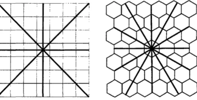
E [eL, (0)] = E [ILs (0) - 1 = E [Ls (0)] - 1 = 1 ,: 0.273. (2.4) By symmetry, we can see that the length bias will be the same for lines whose defining orientation angle lies in the other three quadrants, so the same result is obtained whether we integrate over the full range of angles or merely in the first quadrant. Notice also that we could have limited the integration to the range 0 E [0, 7r/4] since the integrated functions are symmetric about the line 0 = 7r/4. In fact, any of the regions shown in Figure 2-1A serve as a basis for the interval of integration for Equation 2.2, as long as we add absolute value brackets around the sine and cosine functions.' This type of symmetry will be exploited in determining the surface area bias for truncated octahedron and rhombic dodecahedron tilings of space.

Figure 2-1: Bias symmetry regions for square and hexagonal tessellations. The recog-nition of such regions simplifies bias computations in more complicated tessellations. Notice that the hexagonal grid has twelve symmetry regions while the square grid has only eight.

2.3

Hexagonal Tilings

Next consider the errors obtained when the plane is tiled with hexagons, as in Figure 2-2. We start by noticing that for lines of unit length which lie at an angle 0 E [0, 7r/6],

'This 8-way symmetry of the circle with respect to the Cartesian axes is exploited in other domains, such as in the fast Bresenham circle algorithm of computer graphics [4].

the following formula for estimated length holds:

LH (0) = 4 cos 0. (2.5)

The somewhat surprising conclusion is that only the run, and not the rise, of such a line is relevant to the computation of its estimated length! To see this, note that each line which lies in the interval 0 E [0, 7r/6] (L1 and L2 in Figure 2-2) can be estimated by the hexagonal grid pieces in Figure 2-3. Each of these pieces is 4/3 as long as the distance between pixel centers along the x-axis, resulting in Equation 2.5. These hexagonal grid pieces are analogous to the east-west and north-south segments used for computing city block distance on a square grid.

Figure 2-2: Lines on a hexagonal grid. For lines which lie at an angle between

0 E [0, r/6] radians from the x-axis, the estimated length is a constant times the

length of the line projected onto the x-axis.

Unfortunately, the relationship of the hexagons to the coordinate axes becomes fundamentally different when the angle of the line is greater than 7r/6. The line L3 in Figure 2-2 cannot be represented as a sum of the hexagonal grid pieces of Figure 2-3. This leads to a more complex function for estimated length in the region Figure 2-3: These two sections of the hexagonal grid, laid end to end, can be used to approximate any line segment which forms an angle 0 E [0, 7r/6] with the x-axis.

0

[7r/6, r/2]:'

2

2

LH (0) = cos 0 + sin 0. (2.6)

For our mean estimated length for the entire interval 0 E [0, 7r/2], we then have a combination of Equations 2.5 and 2.6:

f 4 cos OdO + (cos 0 + sin 0)d 2 4

6 _{3 3 _ . (2.7)}

f ldO + f 1dO 2

6

Remarkably, this is the same mean length estimate as for the square. Again, in probability notation, we have:

2 2

E [LH (0)]= LH (0) p (0) d=O LH (0) dO= . (2.8)

0 0 2

Our real quarry, however, is the hexagonal length bias which is easily derived from the mean estimated length:

E [eL (0)] = E [ILH (0) - 11] = E [LH (0)] - 1 = - -1

;- 0.273.

While the function for the estimated length of lines with 0 E [rr/6, r/2] is sub-stantially more difficult to derive than for the interval 0 E [0, 7r/6], we note that they result in the same mean estimated length over the separate intervals by examining the numerical values of the integrals in the numerator of 2.7 (they both have mean 4/7r). Looking at the geometry again (Figure 2-1B), we can see that there is symme-try in the hexagon we could have taken advantage of, similar to that of the square. The general mean estimated length (for all angles) can be computed by computing only the mean estimated length for 0 E [0, 7r/6]. All of the symmetry regions which have the same mean estimated length are shown in Figure 2-1B. We emphasize this

2

The derivation of this formula is messy and not of particular interest, so we do not present it here. In fact, we present it mainly to emphasize that we want to avoid computing these types of formulas. Symmetry will be our main tool in avoiding these types of analyses.

point here because using this symmetry will be critical in simplifying surface area bias computations for truncated octahedral and rhombic dodecahedral tilings. Find-ing equations for estimated area over the set of all possible planar segments in three dimensions is substantially more complex than the comparable problem for hexagons in two dimensions.

2.4

Length Bias vs. Centered Length Bias

At first glance, one might conclude that the hexagonal tiling is no better than the square tiling, since they have the same length biases. However, we can make an improvement to our estimated length function on each grid by noticing that the estimated length is almost always3 an overestimate of the true length. We define a new function of the line segment-valued random variable called the centered estimated

length which we define for a square grid as:

cent sin 0 + cos 0

L (0) = Ks (2.10)

where Ks is a correction factor for the overestimate. The centered length error is then

eL~s'ent () = sin

0 +

(2.11)

eehtS. (0) = Ks - 1, (2.11)

such that, for appropriate values of Ks (a little bit larger than 1), eLent. should have a lower mean value than the previously defined error measure. That is, by assuming that the true length of a line segment is a little bit less than the value actually obtained from the local counting algorithm, we are likely to be closer to the true line

3_{For a square grid, the length of segments which align with the coordinate axes will match exactly}

segment length. More formally, the expectation of the centered length error is:

S[e~

nt. (0)]

sin

0

+

cos

0

1

E [en. (9)] = K+s - 1 dO, (2.12)

o s2

which we call the centered bias for the square tiling. We define Ks to be the value which minimizes this expectation. Ks is difficult to obtain analytically due to the ab-solute value within the integral. However, evaluating numerically using a commercial math package [25], we obtain Ks , 1.323, and E [elgt. (0)] - 0.0798 , implying that even after centering, we can expect an error of approximately 8 percent in the length of lines or the perimeter of a figure on a square grid. Summarizing, the integral above represents the mean magnitude of the difference between the true length of the line, which we have defined to be 1, and the centered estimated length.

On a hexagonal grid, the centered estimated length becomes: 4 cos 9

Lcent (0) = s (2.13)

KH

and the centered length error on the hexagonal grid is:

(= 1cos 0

ee. () KH 1 . (2.14) The expected value of this error, the centered bias for the hexagonal grid, is:

E [eLent. (0)] = K -1 d. (2.15)

0

Here, through numerical methods again, we obtain KH / 1.291, and E (Lcnt. (0)) x 0.0348. Hence, tiling with hexagons does improve the mean accuracy of length esti-mates by almost five percent over the square tiling. This corresponds nicely with the intuition that representations with "more circular" pixels (i.e., the hexagonal ones) should demonstrate less sensitivity to line orientation.

2.5

Error Extrema and the Squared Centered Bias

Before moving on to 3-D tessellations, we examine a few more statistics for hexagonal and square tilings, the error extrema and the squared centered bias.

2.5.1

Error Extrema

In many engineering applications, one is concerned with minimizing the worst possible error in measurement. For example, in buying expensive paint to cover an irregularly shaped object, one may want to guarantee that one has enough paint before the project begins. Hence the measurement of the object which produces the smallest maximum possible surface area for a given measured area is desirable. This idea also applies to perimeter estimates.

Suppose we compute the city block distance of a line segment and obtain a value of 1. We do not know the actual length of the line segment which generated this measurement. It could be as short as 1//\2 r- 0.707 and as long as 1. Hence, if we want to prepare for the maximum possible boundary length for a given measurement we need to commit to about 41% more than might actually be needed. For the hexagonal tiling, if a line segment measured 1 according to a local counting algorithm, the actual length would be at least 3/4 and at most V/2. In this case, the maximum is only about 15% greater than the minimum, so the potential for waste is much smaller. Other quantities, such as the expected waste, favor the hexagonal grid. We include in Table 2.1 four statistics related to error extrema for square and hexagonal grids: the minimum and maximum length estimate errors and the minimum and maximum centered length estimate errors. These four quantities give a basic intuition about some of the behaviors of these tilings.

2.5.2

Squared centered error

An alternative to the centered error discussed previously involves weighting large errors more heavily than small errors. To do this we can merely square the residue

used in previous expressions. This gives us

eLsq. (0) sin s - 1 , (2.16) for the square grid, with an expectation of

[eL (9)] =

J

(sin

0

E e. (0)- 1 dO, (2.17)

0 2

which we call the squared centered error.

The value which minimizes the above equation (Ks) represents the "best" ad-justment of our guess at the true length of the line given that we want to weigh larger errors more heavily. By differentiating Equation 2.17 with respect to Ks and setting it equal to 0 we find that the value of Ks which minimizes the expression is r/4 + 1/2 % 1.285, which makes sense, since we expected a value a little greater than 1. And this corresponds to an expected value of exactly 2+2t 6, which is

approximately 0.00946.

For the hexagonal grid, we have an error measure of:

e (cos 0

.(0) = 1)2 . (2.18)

with an expectation of:

E [e. (0)] = cos d. (2.19)

Again, differentiating and equating to 0, we can obtain a value for KH which defines our best guess for true length: KH = + • m 1.275. And again, this is a value slightly greater than 1. This generates an expected value of exactly 2j(3-,r36

which is approximately 0.00176. Thus, for this and higher order weightings of error magnitude, the hexagonal tiling becomes more advantageous.

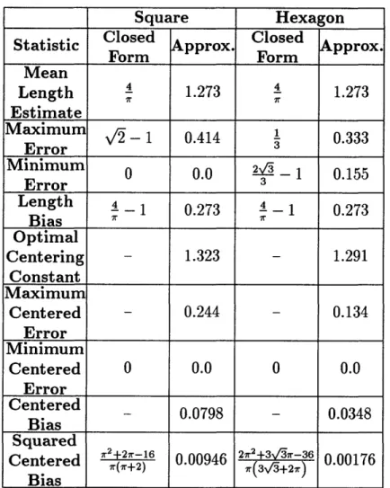
Table 2.1: Some estimated length statistics of a random unit-length line segment process under square and hexagonal tessellations. Notice that while the square and hexagonal grids have equal length bias, the hexagonal grid has a lower centered length bias as well as a smaller range of possible values for length estimates of a unit-length line segment.

2.6

Summary of results for 2-D

Table 2.1 summarizes the results for the perimeter statistics computed in this chapter. While one could compute many other statistics, these capture many of the important practical measures.

Square Hexagon

Statistic Close pprox Clos pprox

Form Form Mean Length 4 1.273 4 1.273 Estimate Maximum _{2- - 1 0.414 1} 0.333 Error 3 Minimum _{0 0.0 2- 1} 0.155 Error 3 Length _{4 1 0.273 4- 1} 0.273

Bias

Centered _{Bias+2) I(3} 2(+27-16 0.00946 2•2+3 ₊₂₎i-36 0.00176

Chapter 3

Three Dimensional Tilings

We now turn to the problem of estimating the surface area of a volume on a discrete grid in three dimensions using a local counting scheme. The basic procedure is for each voxel to report the amount of its own surface area which is part of the surface area of the global object. Measurements of surface area will be biased again due to the discretization of the volume. Just as we assumed in Chapter 2 that planar figures could be well approximated by a finite number of fixed length line segments, we assume in 3-D that the volumes can be well approximated by planar patches or

planar segments of arbitrary orientation and shape but of fixed area. Volumes for

which this is not true are not addressed by the analysis in this paper. For example, fractal surfaces and other highly convoluted surfaces are not subject to the following analyses.

3.1

Cubic Tilings

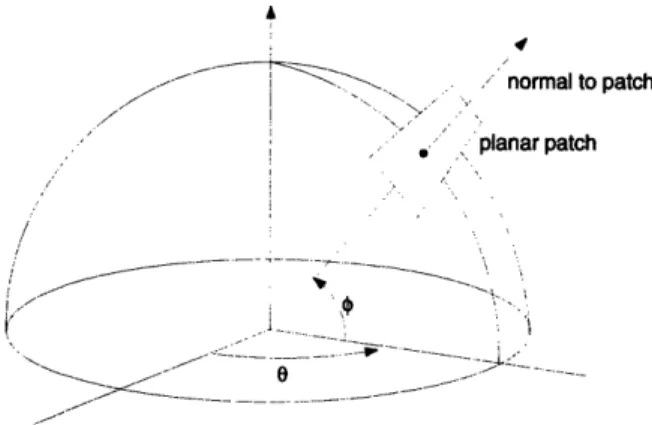
Assume the true area of a planar segment is unity. Let 0 and € define the normal to the planar segment, as one would define a point on the unit sphere by two angles. Such a patch and the associated angles can be seen in Figure 3-1. The estimated area of this planar segment using a local counting algorithm on a cubic grid is then:

assuming (as in the 2-D case with pixels) that the voxel size is small relative to the

normal to patch

planar patch

-- e --.

Figure 3-1: A planar patch and its associated angles.

size of the planar segment. The three terms on the right hand side of Equation 3.1 are the projections of the planar segment onto each of the primary Cartesian planes

(z-y,

block length estimate in two dimensions.

3.1.1

Mean Estimated Area

Integrating Equation 3.1 over the angles 0 and q in the interval [0, 7r/2] and dividing the result by the solid angle (in units of steradians) over which we have integrated gives us the mean area estimate obtained with a cubic grid. We need to multiply the area expression by the Jacobian term, cos €, which handles the foreshortening of area as we approach the "north pole" of the unit sphere.' We have

2 2 _

f+

f Ac (0, ) cos d dO + (sin 0

+

00 Z - 2 (3.2)

2 2 2 2 2

f

J

cos

d dO

f 1d

00 0

We again offer an alternative interpretation of this mean surface area estimate as the expectation of a function of a random process which generates a uniform

'In the terminology of stochastic geometry, we say that the differential form coso do dO is the

density of planar segments tangent to the unit sphere which is invariant under rigid motions of the

coordinate axes. This is hence called the uniform density of this set of planar segments. See [23, page 118].

4=arctan(cos

e)

%0,=0 IO=ic/2

--i/4

Figure 3-2: Integrating the estimated area expression in Equation 3.1 over the spher-ical triangle shown 0 E [0, 7r/2]; 0 e [0, r/2] yields the area bias for planar segments

on a cubic grid. We obtain the same result if we restrict the solid angle of integration

to Area A, B, or C (area A is used in the text).

distribution of planar segments whose normals are distributed equally around the unit sphere. This interpretation yields the stochastic geometry view:

E [Ac (0, )] = . 3 (3.3)

which is simply another framework for interpreting the results in this paper.

In the case of calculating the mean length estimate on a square grid in two dimen-sions, we noted that we could restrict our interval of integration to 0 E [0, 7r/4], due to the symmetry of a square grid. There is an analogous, albeit more complicated symmetry in 3-D on a cubic grid. Picture a sphere whose center is at the origin and whose equator lies in the x-y plane, as in Figure 3-2. The family of planar segments whose normals fall within the solid angle of Area A (or B or C for that matter) of Figure 3-2 have the same estimated areas and hence the same mean estimated area as the total family of planar segments whose normals lie in a single Cartesian octant. That is, just as the range 0 E [0, ir/4] represents all of the unit length line segments needed to calculate the mean estimated length on a square grid, the part of the unit sphere defined by 0 E [0, r/4]; 0 E [0, arctan (cos 0)] represents a family of unit area

planar segments sufficient to calculate the mean estimated area on a cubic grid. To understand this, note that the function we are evaluating (from Equation 3.1) is sym-metric with respect to the three coordinate axes. That is, if we relabel the axes and their associated angles, the value of the function integrated across the entire region remains the same.2 This concept can be tested by integrating the equation for area bias over 1/3 of the spherical triangle shown in Figure 3-2, i.e. the solid angle which is represented by Area A. We should end up with the same mean area estimate which was computed in Equation 3.4, namely, 3/2. We see that this is in fact the case:

7 arctan(cos ) f f Ac (0, €) cos € do dO 0 4- 3 (3.4) arctan(cos 0) -

2

f

f

cos0

do

dO

This symmetry provides us with a slew of identities which can be found in Appendix B. These identities are helpful in deriving closed form solutions to area bias estimates for more complicated tilings which we shall encounter later.

3.1.2

Area Bias, Centered Area Bias, and Other Statistics

Once we have established the area estimation function and calculated the mean area estimate for a tiling, the computations of other statistics for that tiling follow straight forwardly. While it is not always easy to obtain a closed form solution for these statistics, at least numerical approximations can be obtained.

Since we described in detail the various statistics chosen for the square and hexag-onal tilings in the plane, we omit repeating our exposition of these statistics for the cubic tiling, and merely present formulas and solutions for the additional statistics below. These results are summarized in Table 3.1.

2_{Actually, the smallest possible regions of symmetry are half the size of those shown in Figure 3-2.} One can subdivide each of the Regions A, B, and C into smaller regions by drawing a great circle across the sphere from the center of the lune to the corner of the lune. This gives a total of six regions of symmetry per spherical octant, for a total of 48 regions of symmetry on the sphere. The six part symmetry is particularly apparent in Figure 3-11E and Figure 3-11F.

Area Bias for Cubic Tiling

We define the area error to be

eAc (0, 0) =

IAc

3

E [eAc (0, 0)] = E [Ac (0, ) - = E [Ac (0, )] -1 = - 1 = 0.5. (3.6)

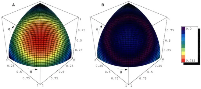
Figure 3-3A shows the area error for a cubic tiling as a function of 0 and €, the two angles which define the normal to a planar segment. The color at each point represents the error for the planar segment defined by that particular point. For the cubic tiling, as expected, the error is zero at the three corners of the plot, since this corresponds to the three principal Cartesian planes, which can be perfectly represented in a cubic tiling. However, as the angle of the plane becomes more oblique, the error increases quickly. The maximum error occurs in the middle of the plot and has an area error of V3- - 1 M 0.732. Figure 3-3B shows the benefit of centering the error which is discussed in the following section.

Centered Bias for Cubic Tiling

To produce the centered area bias, we must first define the centered estimated area to be

A• t " ) Ac(0, €)

A e (t, A)c= ( (3.7)

where Kc is the correction factor for the overestimate of area. Then, the centered

area error is:

eAent. (0, Q) = A ) , 1 (3.8) and the expectation of this quantity is just

T arctan(cos

0)

E

[ea

(0(,

Aent.

K)

1

1 1

Figure 3-3: A. Area error as a function of the planar segment normals 0 and q for the cubic tiling. Notice that the error is zero at the corners which represent the principal Cartesian planes, but increases quickly as we move toward the plane defined by the equation x + y + z = 1, which gives an area error of approximately 0.732. B. Centered area error as a function of 0 and q. The error is greatly reduced by the centering process. The maximum error is now only 0.348 and occurs in the corners of the plot. Notice the purple ring of zero error in the middle of the lune.

Minimizing over Kc using numerical methods, we obtain Ke , 1.533 correspond-ing to a centered area bias of approximately 0.0812. Figure 3-3B shows a plot of the centered area error as a function of the planar segment normals. Notice the greatly reduced error due to the correction factor.

Squared Centered Bias for Cubic Tiling

Following in the same vein, we compute the squared centered error for area, as

$ arctan(cos 0) 2

E

(0,

) =

K

cos

dJ dO,

(3.10)

0 0 6

The value of Kc - 1.516 minimizes the expression, which has a corresponding value of approximately 0.0102.

~~I

0.0

0.732 III •l

Error Maxima and Minima for Cubic Tiling

In two dimensions, computing the values of 0 which maximized and minimized our estimated length functions was easy since these functions are monotonic over the relevant range of 0. In three dimensions, this same statement holds for the partial derivatives (with respect to € and 0) of the cubic grid estimated area function, so again we have it easy:

,Ac (0)=Ac arctan (cos - = v, (3.11)

,10

4

4

and

min

Ac (0, i) = Ac (0, 0) = 1. (3.12) These values give us a maximum centered error of approximately 0.348, and the minimum centered error is of course 0.

3.1.3

Summary of Results for Cubic Grid

Let us pause for a moment to consider the meaning of some of these results. First, the expected error when we simply compute area of a smooth figure on a cubic grid using a local counting scheme is exactly 50 percent. While this is large, we can do substantially better by dividing the result of the local counting algorithm by 1.533 and using this as our guess of the true area. Our expected error is then only about 8 percent, a great improvement. However, as we shall see, we can do substantially better than this. Furthermore, our worst case error, even after centering, is still 34 percent, which is quite severe for some applications. This too, we would like to improve upon.

3.1.4

Other Choices of Grids

Suppose we choose something other than the standard Cartesian cubic grid for our tessellation. Can we reduce the area bias of planar segments represented with different voxels or a different arrangement of voxels? What are reasonable choices for voxel

shapes?

What More Can We Do with Cubes?

Note that even using cubes, we can achieve alternative tessellations with interesting properties by sliding planes of cubes and rows of cubes relative to other planes and rows (Again, this is suggested by Horn [9]). Using cubes we can generate grids which have neighborhood properties equivalent to the truncated octahedron tiling which we explore below. Although we do not investigate the issue here, we conjecture that the surface area bias of a cubic voxel grid arranged in the geometry of a truncated octahedron tiling has greater surface area bias than the corresponding truncated octahedron grid.

Perhaps a more interesting topic for future work would be an analysis of cubic grids with random planar and row-wise displacements. The two dimensional analog would be a brick wall whose successive layers were displaced randomly. We suspect that these configurations may actually be optimal for many problems, but an analysis of these configurations is beyond the scope of this paper.

Affine Transformations of Cubes

Now it is easy to see that any affine transformation of a tessellation is also a tessel-lation. (For more on tessellations, see Appendix A.) We can break these transforma-tions down into translation, rotation, scaling, shearing, and reflection. Translation, rotation, and reflection of grids are not very interesting since they lead to identical area bias analyses. And we already know that the size of pixels and voxels do not affect boundary estimates when the tiles are "small" relative to the tessellated figure (Chapter 2), so scaling our cubic voxels will not yield an improvement in area bias.

Non-uniform scaling of the Cartesian cubic grid yields the interesting case in which the voxels are rectangular prisms, which is probably the most common situation in the data obtained from many sources, including most medical scanners, such as MRI and CT scanners. The somewhat surprising result here is that the area bias for rectangular prism voxels is equivalent to that of cubes. This is easily seen by realizing

that the estimated area function for rectangular prism voxels is the same as that for the cube (Equation 3.1). This seems quite counterintuitive (at least it did to me!). The resolution of this conundrum is that in practice, the largest cubic voxel volume which gives a surface area estimate within some tolerance e will fail to achieve this tolerance for a non-cubic rectangular prism voxel. That is, the voxels must be smaller for rectangular prism voxels to achieve the same performance. However, if we start with the assumption that the voxels are "small enough" which has been our running assumption, then the two tessellations are equivalent.

Tessellations with parallelepipeds are not considered here, but again, we suspect that these will do no better than their correspondingly arranged cubic counterparts. That exhausts the possibilities for cubes and their affine transforms. There are many other groups of polyhedra which tile space however. Some of these can also tile space in more than one manner.

The Regular Polyhedra

There are exactly five regular polyhedra (also called the Platonic solids); they are de-fined as polyhedra in which each face is the same regular polygon[24]. These polyhedra have many properties which make them good candidates for analysis. Unfortunately, among these solids (tetrahedron, cube, octahedron, dodecahedron, and icosahedron), only the cube tiles space, so we have completed our analysis of tessellations for this

class of polyhedra.

The Semi-Regular Polyhedra

Another interesting class of solids are the semi-regular polyhedra. There are various definitions in the literature, but Lyusternik [16, page 147] gives the definition as "a polyhedron all of whose faces are regular polygons (though all faces need not be of the same type) and all of whose polyhedral angles are equal." Properties of these solids and the regular polyhedra can be found in [5, 16, 24].

Of these, three tile space: the triangular prism, the hexagonal prism, and the truncated octahedron. We have chosen to analyze the truncated octahedron here

because of its symmetry properties. An analysis of the prisms seems warranted at some point, however. For now, we turn to the analysis of the truncated octahedron. The hope is that given its more "spherical" shape, it may have less of a centered area bias than the cube.

3.2

The Truncated Octahedron

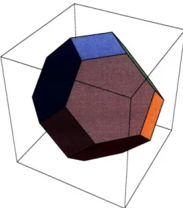
Figure 3-4: A truncated octahedron.

A truncated octahedron (TO) is shown in Figure 3-4. It has 14 sides, eight of which are squares and six of which are regular hexagons. Hence as mentioned before, it is a semi-regular polyhedron. It can be constructed by chopping off (truncating) the corners of a regular octahedron so that the edge length is reduced to 1/3 of the original.

We have already hinted that one may encounter some challenges in evaluating the surface area bias for a TO tiling of space. The primary difficulty encountered is very similar to the one already discussed for the hexagonal tiling of the plane, in which one encounters a fundamental change and increased complexity in the estimation of area for certain orientations of planar segments. In three dimensions the problem is exacerbated by the difficulty of drawing multiple layers of objects. A simple solution to this problem relies again on finding certain symmetries in the tiling which we can