Publisher’s version / Version de l'éditeur:
Vous avez des questions? Nous pouvons vous aider. Pour communiquer directement avec un auteur, consultez la première page de la revue dans laquelle son article a été publié afin de trouver ses coordonnées. Si vous n’arrivez pas à les repérer, communiquez avec nous à PublicationsArchive-ArchivesPublications@nrc-cnrc.gc.ca. Questions? Contact the NRC Publications Archive team at
PublicationsArchive-ArchivesPublications@nrc-cnrc.gc.ca. If you wish to email the authors directly, please see the first page of the publication for their contact information.
https://publications-cnrc.canada.ca/fra/droits
L’accès à ce site Web et l’utilisation de son contenu sont assujettis aux conditions présentées dans le site LISEZ CES CONDITIONS ATTENTIVEMENT AVANT D’UTILISER CE SITE WEB.
2005 ASME Summer Heat Transfer Conference [Proceedings], 2005
READ THESE TERMS AND CONDITIONS CAREFULLY BEFORE USING THIS WEBSITE. https://nrc-publications.canada.ca/eng/copyright
NRC Publications Archive Record / Notice des Archives des publications du CNRC :
https://nrc-publications.canada.ca/eng/view/object/?id=d123902b-93aa-47fd-b486-beefd58209f5 https://publications-cnrc.canada.ca/fra/voir/objet/?id=d123902b-93aa-47fd-b486-beefd58209f5
NRC Publications Archive
Archives des publications du CNRC
This publication could be one of several versions: author’s original, accepted manuscript or the publisher’s version. / La version de cette publication peut être l’une des suivantes : la version prépublication de l’auteur, la version acceptée du manuscrit ou la version de l’éditeur.
Access and use of this website and the material on it are subject to the Terms and Conditions set forth at
On the implementation of stream-wise periodic boundary conditions
Proceedings of HT2005 2005 ASME Summer Heat Transfer Conference July 17-22, 2005, San Francisco, California, USA
HT2005-72271
ON THE IMPLEMENTATION OF STREAM-WISE PERIODIC BOUNDARY CONDITIONS
Steven B. Beale
National Research Council Montreal Road
Ottawa Ontario K1A 0R6 Canada steven.beale@nrc-cnrc.gc.ca
ABSTRACT
Fully-developed periodic boundary conditions have frequently been employed to perform calculations on the performance of typical elements of heat exchangers. Many such calculations have been achieved by transforming the equations of motion to obtain a new set of state variables which are cyclic in the stream-wise direction. In others, primitive variables, based on substitution schemes are employed. In this paper; a review of existing procedures is provided, and a new method is proposed. The method is based on the use of primitive variables with periodic boundary conditions combined with the use of slip values. Either pressure difference or mass flow rate may be prescribed, and both constant wall temperature and constant heat flux wall conditions may be considered. The example of an offset-fin plate-fin heat exchanger is used to illustrate the application of the procedure. The scope and limitations of the method are discussed in detail, and the mathematical basis by which the method may be extended to the consideration of problems involving mass transfer, with associated continuity, momentum, and species source/sinks is proposed.
INTRODUCTION
In the application of computational fluid dynamics to heat exchanger design, it has long been recognized that much computational effort may be spared by considering elements deep within the design where the flow is ‘fully-developed’; for example; Thom and Alpelt [1], LeFeuvre [2], and Massey [3] considered fully-developed flow in tube banks assuming a cyclical 2-D stream function/vorticity formulation. In [2,3] temperature was also solved-for.
More recently, the equations of motion are usually solved in terms of primitive variables, for which the steady-state form is typically written, subject to certain simplifications, as:
( )
0divρu = , (1)
(
u;u)
grad div(
gradu)
divρ =− p+ µ (2)
(
cp T)
div(
kgradT)
divρ u = (3)
For convenience, and without loss of generality it is assumed that the region has been tessellated with a structured mesh with associated finite-volume equations [4]:
(
)
(
)
(
)
(
)
(
φ −φ)
+(
φ −φ)
+ =0 + φ − φ + φ − φ + φ − φ + φ − φ S a a a a a a P H H P L L P N N P S S P E E P W W (4) where φ=p,u,v,w,T is a general state-variable, and the well-known compass notation [4] has been employed. The source-term in Eq. (4) is frequently linearized according to(
V P)
CS = −φ (5)
where S is referred to as a source-term coefficient and V is a source-term value.
A problem frequently encountered is that it is difficult to construct a mesh large enough to describe the gross motion of the fluid within the entire heat exchanger, and yet fine enough to capture the boundary-layer detail around individual elements [5,6]. Often a single ‘typical’ module, or perhaps a small group of such modules, is considered, with the flow taken as being ‘fully-developed’ in the stream-wise direction,
(
0,y,z) (
ul,y,z)
u = (6)
(
0,y,z) (
pl,y,z)
p0p = +∆ (7)
where ∆p0 is the pressure drop over characteristic length, l.
NOMENCLATURE
A Area, m2
a Coefficient in finite-volume equation
B Mass transfer driving force
b Width, m
C Value in linearized source term cp Specific heat, J/kgK
f Friction factor
j Heat transfer factor
k Thermal conductivity, W/mK
l Length, m
Proceedings of HT2005 2005 ASME Summer Heat Transfer Conference July 17-22, 2005, San Francisco, California, USA
T Temperature, K
u Stream-wise velocity component, m/s
v Cross-wise velocity component, m/s
w Cross-wise velocity component, m/s p Pressure, Pa, pitch, m
V Value in linearized source term
Vp Volume of cell P, m3
x Stream-wise displacement component, m
y Cross-wise displacement component, m
z Cross-wise displacement component, m Greek Letters
β Volumetric term δ Fin thickness
φ Generalized state variable Γ Exchange coefficient, kg/ms θ Non-dimensional temperature ρ Density, kg/m3 σ Volumetric term τ Characteristic time, s ω Weighting factor
REVIEW OF PREVIOUS WORK Transformed variable approach
Patankar Liu and Sparrow [7] transformed the state-variables to a set of equations which were truly cyclic in the sense:
(
x,y,z) (
=φx+l,y,z)
φ (8)
This was achieved in the momentum equations by defining a ‘reduced’ pressure, ~p, according to:
x p p= −β
~ (9)
where β=∆p0 l and ∆p0=p0
( )
0 −p0( )
l is a referencepressure difference. The reduced pressure, p~, is thus cyclic in the sense of Eq. (8); the pressure, p, may be obtained algebraically at the end of the computational cycle, if required. The momentum equation may readily be written in the form,
(
u;u)
ˆ grad~ div(
gradu)
divρ =βi− p+ µ (10)
Thus when solving for p~, a volumetric source term,
p
V
S=β is introduced into the x-direction momentum
equation. Pressure gradient, as opposed to mass flux or Reynolds number must be prescribed. Subsequently, Murthy and Mathur [8] suggested a rationale whereby β may be systematically adjusted until the desired mass flux is obtained.
For heat transfer at constant wall flux, qwall'', an
essentially similar situation exists with,
0 ) , , ( ) , , (x y z T x l y z T T = + +∆ (11)
A reduced temperature, T~, may be defined as,
x T
T~= −γ (12)
where γ=∆T0 land T ~
is cyclic. The transformed energy equation is:
(
cp T)
u(
k T)
~ grad div ~ divρ u + γ= (13)and a source term S =−uγVp is introduced in the energy
equation.
For constant wall temperature Twall, a non-dimensional
temperature, θ, may be defined as;
wall 0 wall T T T T − − = θ (14)
where T0(x) is some suitably-defined module reference
temperature; for example, the local bulk temperature at x. The
non-dimensional form of the energy equation with θ as state-variable is less straightforward
(
ρ θ)
=div(
gradθ)
+σ div ucp k (15) where wall 0 2 0 2 wall 0 0 2 T T x d T d c k T T x d dT u x c k p p − θ ρ − − θ − ∂ θ ∂ ρ = σ (16)These various implementations have been adopted by numerous researchers, for example Patankar and Prakash [9], and at least one commercial CFD code has been modified to allow for solutions to equations of the form (10)-(16) to be incorporated for stream-wise periodic problems. The reader will note that it is necessary to modify wall boundary conditions in the reduced form of the transport equations, see [7] for details.
Because of the additional complexity associated with the solution of Eqs. (15) and (16); alternative formulations, Kelkar and Patankar [10], have been proposed based on a primitive-variable formulation, for constant Twall problems. In this paper,
all solved-for variables are primitive variables, regardless of the choice of wall boundary conditions.
Primitive variable approach
The present author did not adopt the methodology [7] but instead worked directly with the primitive variables, p, u, v, w, T, in previous work [11-13]. The reasons for this were as
follows: (a) There is no need to introduce new state-variables: (b) Reynolds’ number can be directly stipulated; (c) Constant
Twall boundary conditions may readily be prescribed; (d) Flow
symmetry may be exploited for staggered or offset geometries, halving the required number of grid cells. In the primitive formulation, the temperature, T, is given by,
(
0,y,z)
c1T(
l,y,z)
c2 T = + (17) where( )
( )
(
)
( )
( )
− − = − − = wall 0 0 wall 1 wall 2 wall wall wall 0 wall 0 1 ' ' constant 0 constant 1 ' ' constant 1 constant 0 q T L T T c Τ c q T T L Τ T Τ c (18)The periodic boundary conditions were implemented by the addition of an additional line of ‘halo’ cells downstream, at
1 + = nx
Antonopoulos [14-16]. This approach was employed because non-standard grids, which could not readily be connected together in a structured manner, were employed.
Downstream velocity and temperature values were substituted upstream in the continuity, momentum, and energy equations in the normal sense as convected inlet boundary values; temperatures being scaled according to Eq. (17). The downstream pressure values at i= nx+1 were fixed to the upstream values as p
(
nx+1,j) ( )
=p1,j −p0. The meanpressure at i=1 was chosen as the reference pressure, p0; and
thus ensured that the mean downstream pressure was zero, as the upstream values rose to some finite value. In addition the upstream velocity profile was scaled so as to render the desired overall Reynolds number. This scheme corresponded to the common practice of prescribing upstream boundary values and fixing the outlet pressure. The early methodology presumed no re-circulation to occur at the upstream/downstream boundaries; a situation sometimes referred to as ‘locally parabolic’ [4]. This requirement was subsequently relaxed by means of a double-substitution process whereby upstream values of velocity and temperature were also substituted downstream [12,13].
One advantage of the use of primitive variables is that transient problems may also be considered [17];
(
0,y,z,t) (
=ul,y,z,t+τ)
u (19)
(
0,y,z,t)
c1T(
l,y,z,t)
c2T = +τ + (20)
In that case, downstream values were stored in a ‘ring-buffer’ and substituted upstream after time τ (substantially longer than the characteristic period of oscillation of the system) has elapsed. This allowed-for span-wise amplification of small periodic oscillations (vortex-shedding, wake/shear layer instabilities) to be successfully replicated.
The use of periodic boundary conditions is not confined to heat transfer problems. Comini and Croce [18] considered periodic mass transfer in tube-fin heat exchangers under conditions of prescribed wall value, based on local saturation conditions for an ideal gas mixture. Beale [19] considered fully-developed mass transfer in plane and square ducts. The velocity and scalar profiles were presumed similar according to
( )
cu( )
lu0 = (21)
with v
( ) ( )
0 =vl and w( ) ( )
0 =wl ; the upstream bulk velocity being fixed to some value u0.For scalar transport, a constant transformed substance-state boundary condition, as opposed to constant wall flux or constant value, was presumed. Periodicity is imposed with
( )
0 =c1φ( )
l +c2φ (22)
by computing c1=
(
φb( )
0 −φw( )
0) ( )
(
φb l −φw( )
l)
and( )
c( )
lc2=φw 0 − 1φw in a manner analogous to Eq. (17). The
upstream wall value must be computed,
( )
(
b( ) ( )
Bl t)
(
B( )
l)
w = φ + φ +φ 0 0 1 , where B is a mass transfer
driving force [20].
PRESENT CONTRIBUTION
The problem addressed in this paper is the means whereby periodic boundary conditions may be reduced to cyclic conditions in the primitive-variable formulation, without the cumbersome step of introducing ‘halo’ cells. The solution is achieved by imposing ‘slip’ boundary conditions at the grid
edges in the x-direction. Slip boundary conditions are naturally
encountered, for example in the temperature field in radiative heat transfer problems, and elsewhere.
Momentum equation
No special treatment is required in the continuity (pressure correction) equation, or the cross-wise v and w momentum
equations. For stream-wise u-momentum the situation is
extremely simple: All that is required is that a constant step be imposed as a force corresponding to the overall pressure change
0
p A
S = P∆ (23)
along a single y-z plane of cells. The pressure slip may be
applied at any location in the domain, however if it is applied at the system boundary, i = nx, there is the superficial advantage
that graphical post-processing software may not interpolate between the two values, producing spurious bands of iso-values within the computational domain. Figure 1(a) illustrates the notion schematically, for the case of a staggered scheme [21]. The in-cell pressure must also be fixed, elsewhere, to some reference value at one cell in the computational domain, in order to prevent the pressure field from wandering.
If it is desired that the bulk velocity, u , or Reynolds’ number, be prescribed; the imposed pressure difference, ∆p0,
may be adjusted: ' * 0 0 0 p p p =∆ +∆ ∆ (24)
where ∆p0*is the value of the pressure difference at the
previous iteration, and ∆p0'is a pressure correction. Since in
the SIMPLE algorithm [22] ue=b
(
pP'−pE')
where Ee P e p A a u
b=∂ ∂ = , it may be concluded that,
(
)
∑
∑
−=
∆p0' ae u ue* Ae or ∆p0'=R
(
u−ue*)
. The choiceof R is not critical, and need only be sufficiently accurate as to
procure rapid convergence. Neglecting stream-wise diffusion and applying an order of magnitude analysis yields the following simplified relation;
(
*)
'0 u u u
p =ρ −
∆ (25)
which is identically true in the lim u*→u. This methodology is similar to, but simpler than that given in ref. [8].
Heat transfer
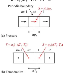
For the temperature field there is a slip; not in the flux or source, but in the actual value across the boundary faces: A different treatment is required: It is necessary to prescribe a source/sink pair. The reader will note that these are not necessarily equal and opposite, owing to the well-known non-linear property of the convection-diffusion system of equations [4].
Various means to code the slip temperatures at x = 0 and x = l. are available; (i) If the user has access to the neighbor
values, φW and φE, in the finite-volume equation, Eq. (4); it will
be possible to directly add/subtract the ∆T slip-values, from the neighbors, TE and TW. (ii) If, however, the user does not
have access to the neighbor values, as is more often the case, then it is convenient to introduce a pair of linearized source terms:
(
W P)
W T T a(
E P)
E T T aS= ∆ − at i = nx (27)
Figure 1 Slip boundary conditions for a staggered scheme, constant wall flux, .
where the slip values, ∆TW and ∆TE, are the differences
between the actual temperatures and the ‘apparent’ temperatures that would arise if the field were truly periodic. If
W T
∆ is positive then ∆TE is negative, and vice-versa.
These source terms are easily coded simply by setting
C = anb and V = ∆Tnb in Eq. (5) where the subscript ‘nb’ refers
to the east or west neighbor value. The linking coefficients aE
and aW must be computed using exactly the same scheme
employed in the CFD solver.
For the case of constant wall flux, qwall'', the temperature
difference is constant, ∆TW =∆T0, ∆TE=−∆T0, and Fig. 1(b)
illustrates schematically the coding of the source-sink pair. It is, in theory, possible to directly obtain ∆T0=q mcp[7], and code
this as a fixed flux (source): However, the in-cell temperature must then be prescribed to a constant value at some chosen location, T = Tref, as above. The temperature (enthalpy) slip
must precisely balance the net heat flux at the wall. If there is even the slightest error in the value of the computed value of
0
T
∆ , e.g. for complex geometry, the error will be manifested as distortion in the region near the cell with fixed temperature. For this reason the author chooses to prescribe the temperature as a linearized source term; for example C=aW and
0
T
V =±∆ , upstream in Eq. (5). The source-term value is adjusted iteratively until the upstream in-cell temperature reaches the desired reference value,
( )
T( )
l TT0= 0 0 − 0
∆ (28)
In other words T0(l) is a fetched-value of T at some chosen
location, or the mean-value downstream, during the iterative cycle, whereas T0(0) is a constant value prescribed by the user
(e.g. T0 = 0).
For the case of constant Twall, ∆TE≠−∆TW, the
implementation is similar to that in [10]. It is readily apparent that the temperature slip may be obtained from,
( )
( )
wall wall 0 0 0 wall ( ) 0 T T T T l T T l T T T T W W E E − ∆ − = − − = − ∆ (29) From whence the source-term values for the general case may be written as;(
c1 1)
T c2V = − W+ at i = 1 (30)
(
1 c1)
T c2V = − E− at i = nx (31)
where TW is the west neighbor at i = 1 (i.e. TP at i = 1) and TE is
the east neighbor at i = nx (i.e. TP at i = 1). Once again, the
source-term coefficients in Eq. (5) are just aW and aE.. Eqs. (30)
and (31) may be written in compact form as
(
1 c1)
Tnb c2V =± − ∓ .
CASE STUDY: OFFSET-FIN HEAT EXCHANGER
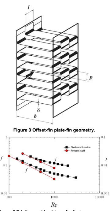
The problem considered to illustrate the methodology is that of fully-developed conjugate heat transfer in a 3-D offset-fin plate-offset-fin heat exchanger under laminar flow conditions. Numerical solutions to this problem were previously presented in [11,12] using the ‘halo’ cell method. Figure 3 shows the geometry. The design selected was Core 105 from Shah and London [23,24]. Two plates separated by a distance b are
considered to be at constant wall temperature Twall. A
rectangular strip-fin, length, l, thickness δ, is offset at pitch, p.
A computational domain of 2l×p/2×b corresponding to two
complete modules was constructed. Geometry and properties are given in Tables 1 and 2, respectively.
The flow Reynolds number was prescribed and the resulting ∆p0 adjusted according to Eq. (25). Temperature slip
was prescribed according to Eqs. (30) and (31) with the constants c1 and c2 computed according to Eq. (18). Figures 2,
4, and 6 display velocity vectors, pressure and temperature contours for plan and elevation views of the heat exchanger.
Overall friction and heat transfer factors are computed according to 2 0 2 b h u l p D f ρ ∆ = (32)
( )
1 3 2 ln Pr c A A j= c (33)where Ac =
(
b−2δ)(
p−δ)
is the minimum free-flow area and(
−δ)
+(
−δ)
+ δ+(
−δ)
δ= lb l p b p
A 2 2 2 is the area for heat
transfer. These are compared to experimental values in Fig. 5. It can be seen that agreement in the laminar flow regime is quite good.
Figure 2 Velocity vectors, Re = 500.
Figure 3 Offset-fin plate-fin geometry. Figure 4 Pressure contours, Re = 500.
Figure 5 Friction and heat transfer factors compared with available experimental data.
Figure 6 Temperature contours, Re = 500.
Table 1. Dimensions for Core 105. Table 2. Fluid properties.
Quantity Value (mm) b 1.905 p 1.054 l 2.822 δ 0.1016 Quantity Value ρf 0.9944 (kg/m 3 ) µf 20.82x10 -6 Pa.s k 0.03035 W/mK cp 1.016 x10⁻³ J/kg.K
DISCUSSION
The results show that it is possible to code stream-wise periodic problems in primitive form with cyclic boundary conditions, by the selective introduction of slip boundaries. For problems involving fluid mechanics and heat transfer, the approach proposed in this work offers the advantages that storage does not require to be allocated for additional ‘reduced’ variables. Moreover the implementation of the slip boundary value is essentially replicating, in a mathematical manner, that which occurs naturally. It is true that the slip conditions must be coded, but this is offset by the fact that the wall boundary conditions are in the standard form, i.e. do not require modification.
Of course it might be argued that even if Eqs. (15) and (16) are somewhat inelegant; provided the implementation of reduced variables is hidden from the user, the means is inconsequential to the engineer; so long as a correct solution is obtained. Notwithstanding the above, the primitive variable formulation is easy to code and offers clear advantages, not only for the constant wall temperature problem, but potentially for fully-developed mass transfer problems.
The reader will note for the case of locally-parabolic flow at sufficiently high Reynolds number; upstream
w PuA T c
S=ρ ∆ , and downstream S=0 as expected. For the case of pure conduction; S=ΓA
(
∆T−Tp)
δx, both upstreamand downstream. The reader will note that for constant Twall the
∆T slip values are not necessary equal on either side of the boundary.
The simple method devised to adjust the pressure jump based on a desired reference bulk velocity or Reynolds number, as given in Eq. (25), was found to work well for the problem under consideration, and others (not shown).
Choice of reference values
The choice of reference value, φo, is not exclusive; One
obvious possibility is that of the weighted mean value at x = L,
∫
∫
ω ωφ = φ A A dA dA 0 (34)where ω is a weighting factor. The most commonly-used weighting factor is the velocity, ω=u, i.e., the so-called bulk value, φ0 =φ. It has also been suggested [7] that for
re-circulating flows a more appropriate weighting in Eq. (34) is velocity magnitude ω=u; a discussion of some of the issues may be found in [12]. For computing a reference pressure, p0,
the weighting factor would normally be unity.
Another basis for the reference value, φo, is a module
average value,
∫ ∫
∫ ∫
φ = φ l A l A dx udA dx dA u 0 0 0 (35)Another very convenient reference φo, is the in-cell value at
some particular location, say j = j0, k = k0. Finally it is worth
noting that φo, need not correspond to any particular x-location;
i.e., it could be at some offset i = i0+n. Provided a consistent
practice is adopted, there is a great deal of flexibility in the choice of φ0. In other words, the choice of weighting factor is
rather arbitrary, but is usually chosen to correspond to some well-established norm in fluid mechanics or heat transfer.
Mass transfer
There are numerous problems involving mass transfer with finite wall velocity, vwall. A fully-developed periodic condition
with a similarity velocity profile, u
( )
0 =cu( )
l can be presumed, wherec=u0( ) ( )
0 u0l . Putting( )
( )
wall flow wall 0 0 0 0 v A A l u u u = − = ∆ (36)In the continuity (pressure-correction) equation, a single constant sink equal and opposite to the overall mass source (or vice-versa) at the wall is required:
(
c) ( )
ul Au A
S=−ρ w∆ =−ρ w −1 (37)
In the u-momentum equations it is also necessary to
introduce a velocity slip, analogous to the temperature slip, on either side of the continuity cells for which Eq. (37) is applied,
(
c 1)
unbV=± − (38)
The momentum equations may further be complicated by the fact that the source-term coefficients may also need to be corrected.
With these modifications; future work will include examples of 3-D fully-developed periodic mass transfer problems: Previous works on this subject by other authors [18,25] were primarily for low mass flow rates; where no continuity modifications were implemented. At higher mass flow rates injection/suction rates have a significant impact on the v-velocity, pressure gradients and scalar transport, which
cannot be captured merely by neglecting the impact on continuity of mass transfer. While it might, in theory, be possible to incorporate these effects by defining a ‘reduced velocity’ satisfying a cyclic form, Eq. (8), for continuity; the resulting momentum equation will contain quadratic terms and may not therefore be readily amenable to such a treatment.
CONCLUSIONS AND FUTURE WORK
Periodic boundary conditions may readily be coded, based on a primitive variable formulation for fluid mechanics and heat transfer problems. This is achieved by combining cyclic boundary conditions with the use of slip values. The latter are introduced as linearized source terms.
The methodology has the advantages that no new variables need be introduced, and that standard wall boundary conditions may be used. Moreover it corresponds physically to the actual situation at hand. It may readily be implemented in existing CFD codes with only minor modifications. Either a mean pressure gradient, or a reference velocity/flow Reynolds number may be prescribed using a simple algorithm.
Although the work presented here was based on a finite-volume method, with a structured mesh, and employing a staggered scheme; the technique is quite general and may
readily be applied to; unstructured meshes, schemes employing co-located variables, and other methodologies such as finite-element analysis. The technique will be extended in the future, to consideration of engineering problems involving mass transfer under constant transformed substance state with associated variation in the continuity, momentum, and species fields.
ACKNOWLEDGMENTS
Dr. John Ludwig at CHAM Ltd. provided assistance with the computer code used to generate the results. Mr. Ron Jerome of NRC provided general technical support. Dr. Katherine Cooke assisted in a literature survey. The support of the National Research Council is gratefully acknowledged.
REFERENCES
[1] Thom, A., and Apelt, C. J., 1961, Field Computations in Engineering and Physics, Van Nostrand, London.
[2] Le Feuvre, R. F., 1973, "Laminar and Turbulent Forced Convection Processes through in-Line Tube Banks." Ph.D. thesis, Imperial College, University of London.
[3] Massey, T. H., 1976, "The Prediction of Flow and Heat-Transfer in Banks of Tubes in Cross-Flow." Ph.D. thesis. [4] Patankar, S. V., 1980, Numerical Heat Transfer and Fluid Flow, Hemisphere, New York.
[5] Spalding, D. B., 1981, "Methods of Calculating Heat Transfer within the Passages of Heat Exchangers", Computational Fluid Dynamics Unit, Imperial College, University of London, HTS/81/4, London.
[6] Spalding, D. B., 1981, "The Calculation of Heat-Exchanger Performance", Computational Fluid Dynamics Unit, Imperial College, University of London, HTS/81/5.
[7] Patankar, S. V., Liu, C. H., and Sparrow, E. M., 1977, "Fully-Developed Flow and Heat Transfer in Ducts Having Streamwise-Periodic Variations of Cross-Sectional Area." Journal of Heat Transfer (Transactions of the ASME), 99, pp. 180 -186.
[8] Murthy, J. Y., and Mathur, S., 1997, "Periodic Flow and Heat Transfer Using Unstructrured Meshed", International Journal for Numerical Methods in Fluids, 25, pp. 659-677. [9] Patankar, S. V., and Prakash, C., 1981, "An Analysis of the Effect of Plate Thickness on Laminar Flow and Heat Transfer in Interrupted Plate Passages", International Journal of Heat and Mass Transfer, 24, pp. 1801-1810.
[10] Kelkar, K. M., and Patankar, S. V., 1987, "Numerical Prediction of Flow and Heat Transfer in a Parallel Channel with Staggered Fins", Journal of Heat Transfer, 109, pp. 25-30. [11] Beale, S. B., 1990, "Laminar Fully Developed Flow and Heat Transfer in an Offset Rectangular Plate-Fin Surface", PHOENICS Journal of Computational Fluid Dynamics and its Applications, 3, pp. 1-38.
[12] Beale, S. B., 1993, "Fluid Flow and Heat Transfer in Tube Banks", PhD thesis, Imperial College of Science, Technology and Medecine, London.
[13] Beale, S. B., and Spalding, D. B., 1998, "Numerical Study of Fluid Flow and Heat Transfer in Tube Banks with Stream-Wise Periodic Boundary Conditions", Transactions of the CSME, 22, pp. 394-416.
[14] Antonopoulos, K. A., 1979, "Prediction of Flow and Heat Transfer in Rod Banks", Ph.D thesis, Imperial College, University of London.
[15] Antonopoulos, K. A., 1985, "Heat Transfer in Tube Assemblies under Conditions of Laminar, Axial, Transverse and Inclined Flow", International Journal of Heat and Fluid Flow, 6, pp. 193-204.
[16] Antonopoulos, K. A., 1987, "The Prediction of Turbulent Inclined Flow in Rod Banks." Computers and Fluids, 14, pp. 361-378.
[17] Beale, S. B., and Spalding, D. B., 1999, "A Numerical Study of Unsteady Fluid Flow in in-Line and Staggered Tube Banks", Journal of Fluids and Structures, 13, pp. 723-754. [18] Comini, G., and Croce, G., 2001, "Convective Heat and Mass Transfer in Tube-Fin Exchangers under Dehumifying Conditions", Numerical Heat Transfer, Part A, 40, pp. 579-599.
[19] Beale, S. B., 2005, "Mass Transfer in Plane and Square Ducts", International Journal of Heat and Mass Transfer, 48, pp. 3256-3260.
[20] Spalding, D. B., 1960, "A Standard Formulation of the Steady Convective Mass Transfer Problem", International Journal of Heat and Mass Transfer, 1, pp. 192-207. [21] Harlow, F. H., and Welch, J. E., 1965, "Numerical Calculation of Time-Dependent Viscous Incompressible Flow of Fluid with Free Surface." The Physics of Fluids, 8, pp. 2182-2189.
[22] Patankar, S. V., and Spalding, D. B., 1972, "A Calculation Procedure for Heat, Mass, and Momentum Transfer in Three-Dimensional Parabolic Flows", International Journal of Heat and Mass Transfer, 15, pp. 1787-1806.
[23] Shah, R. K., 1967, "Data Reduction Procedures for the Determination of Convective Surface Heat Transfer and Flow Friction Characteristic Steam-to-Air Test Cores", Department of Mechanical Engineering, Stanford University, Stanford. [24] Shah, R. K., and London, A. L., 1967, "Offset Rectangular Plate-Fin Surfaces - Heat Transfer and Flow Friction
Characteristics", Deptarment of Mechanical Engineering, Stanford University.
[25] Baier, G., Grateful, T. M., Graham, M. D., and Lightfoot, E. N., 1999, "Prediction of Mass Transfer in Spatially Periodic Flows", Chemical Engineering Science, 54, pp. 343-355.