The use of thermogravimetry to analyze a mixed plastic waste stream

Publisher’s version / Version de l'éditeur:

Journal of Thermal Analysis, 42, 2-3, pp. 397-424, 1994-08

READ THESE TERMS AND CONDITIONS CAREFULLY BEFORE USING THIS WEBSITE.

https://nrc-publications.canada.ca/eng/copyright

Vous avez des questions? Nous pouvons vous aider. Pour communiquer directement avec un auteur, consultez la première page de la revue dans laquelle son article a été publié afin de trouver ses coordonnées. Si vous n’arrivez pas à les repérer, communiquez avec nous à PublicationsArchive-ArchivesPublications@nrc-cnrc.gc.ca.

Questions? Contact the NRC Publications Archive team at

PublicationsArchive-ArchivesPublications@nrc-cnrc.gc.ca. If you wish to email the authors directly, please see the first page of the publication for their contact information.

NRC Publications Archive

Archives des publications du CNRC

This publication could be one of several versions: author’s original, accepted manuscript or the publisher’s version. / La version de cette publication peut être l’une des suivantes : la version prépublication de l’auteur, la version acceptée du manuscrit ou la version de l’éditeur.

For the publisher’s version, please access the DOI link below./ Pour consulter la version de l’éditeur, utilisez le lien DOI ci-dessous.

https://doi.org/10.1007/BF02548524

Access and use of this website and the material on it are subject to the Terms and Conditions set forth at

The use of thermogravimetry to analyze a mixed plastic waste stream

Day, M.; Cooney, J. D.; Fox, J. L.

https://publications-cnrc.canada.ca/fra/droits

L’accès à ce site Web et l’utilisation de son contenu sont assujettis aux conditions présentées dans le site LISEZ CES CONDITIONS ATTENTIVEMENT AVANT D’UTILISER CE SITE WEB.

NRC Publications Record / Notice d'Archives des publications de CNRC:

https://nrc-publications.canada.ca/eng/view/object/?id=ded05c91-1229-4214-8af6-268b440ce3a6 https://publications-cnrc.canada.ca/fra/voir/objet/?id=ded05c91-1229-4214-8af6-268b440ce3a6

Journal of Thermal Analysis, Vol. 42 (1994)397-424

THE USE OF THERMOGRAVIMETRY

TO ANALYZE A MIXED PLASTIC

WASTE STREAM"

M. Day, J. D. Cooney and J. L. Fox

Institute for Environmental Chemistry, National Research Council Canada, Ottawa, Ontario, Canada, K1A OR6

A b s t r a c t

The thermogravimetry of a mixed polymer waste stream has been studied and the weight-loss behaviour of this heterogeneous mixture has been compared with results obtained from the weight-loss curves of some individual polymers. The results suggest that the behaviour of the mixture cannot be predicted by the simple additive behaviour of the individual polymers since interactions can occur which influence the degradation weight-loss profiles. The heterogeneous polymeric waste studied was that generated from the shredding of old discarded automobiles. The results of the study indicate that while it is possible to determine what is present in a sample, the relevance of the data to a very heterogeneous waste stream is questionable.

Keywords: polymers, TG I n t r o d u c t i o n

Plastic recycling in the US is currently quite small (5%) but has been fore- cast to grow dramatically, especially for rigid containers, over the next few years [1] as a result of increased public awareness and political regulatory pres- sure. In order to expand the recycling of plastics, there are many economic and technological problems that need to be addressed [2-4] such as viable markets, cost recovery, product purity, sortation efficiency, product performance, etc.

One of the fundamentals of any process is quality control. It is good practice in any process to determine the chemical and physical properties of the raw ma- * Issued as NRCC #37562

0368--44661941 $ 4.00 John Wiley & Sons, Limited

398 DAY ct al.: PLASTIC WASTE STREAM

terials to be used in the process to ensure that they meet the specifications re- quired to obtain a satisfactory product. The processing of recycled plastics should be no different. Before recycling a mixed waste stream, a procedure should be developed to "characterize" in a sound and scientific way, the poly- meric components in the waste stream.

In this study we have examined the waste known as Auto Shredder Residue (ASR) generated by metal shredding operations in North America. In the shred- ding process an old automobile hulk is fed into a hammermill where the com- ponents are reduced in size to fist size pieces of material before being separated into a metallic ferrous stream, a metallic non-ferrous stream and a light "fluff" fraction referred to as ASR. While the two metallic fractions are recycled, the remaining commingled ASR waste is usually landfilled. The shredding of a 1979 North American automobile weighing approximately 1500 kg would, on average, yield 1100 kg of ferrous metal and 250 kg of ASR [5]. The ASR typi- cally consists of a wide range of materials including plastics, rubber, foam, tex- tiles, wood, glass, rust, dirt, etc. contaminated with oil, fluids and metal fragments [6]. Clearly this waste stream is not of a precise composition with the materials present and their concentrations being greatly dependent upon the make, model and year of the automobiles being fed into the shredder. In a pre- vious study, we performed a detailed characterization of this material employ- ing a systematic and scientific protocol [7]. This study provided some valuable information on the typical composition of this heterogeneous waste stream, along with an indication of the type and magnitude of sample variability that could be expected. This study not only provided some valuable information on the composition of the material, but based upon data from other studies [8] has indicated that the sampling procedure employed was acceptable and repeatable [91.

The object of the present study was to investigate the use of thermo- gravimetry (TG) to provide information on the polymeric composition of this mixed plastic waste stream known as ASR.

E x p e r i m e n t a l

Four automotive polymeric samples were employed in this study along with the ASR. They included:

- Himont's PRO-FAX SV-152 polypropylene copolymer recommended for automotive applications (designated PP)

- Dow's Magnum Acrylonitrile/Butadiene/Styrene plastic resin recom-

mended for interior automotive components (designated ABS) - BF Goodrich's Geon, polyvinyl chloride (designated PVC)

DAY et al.: PLASTIC WASTE STREAM 399

- An automotive polyurethane foam received from Curon Canada Ltd, sup- pliers to the auto industry (designated PU).

All the above polymers were ground in the presence of liquid nitrogen using a Wiley Laboratory Mill to a size less than 20 mesh (1 mm) prior to use. Mix- tures of these polymer powders were then obtained by blending appropriate amounts of the individual polymers together to give mixtures with the appropri- ate composition required for analysis.

The ASR samples used in this study were collected using a scientifically ac- cepted sampling protocol to ensure that samples brought to the laboratory for analysis were representative of the material being produced by shredding opera- tions in the provinces of Ontario and Quebec, Canada [7]. The actual process involved collecting approximately 1-2 tonnes of ASR that was produced from at least 15 automobiles. This material was transferred to a concrete pad where it was reduced in size to 50 kg by a cone and quartering procedure. This re- duced representative sample was bagged, labelled and transferred to the labora- tory for subsequent analysis. Four such representative samples were obtained from each participating shredding operation. In this study samples from 3 shredding operations were employed.

In the laboratory these test samples were further subdivided into test speci- mens which were then homogenized using a Startevant Laboratory Roll Crusher (IR46) followed by a Wiley Laboratory Mill (Model 4) to a size less than 2 mm (liquid nitrogen was employed during this size reduction process).

Representative experimental test sub-specimens of the ASR, suitable for use in the TG experiments, were obtained from the homogenized test specimens by the use of a riffle funnel.

The thermal analysis experiments were performed on a TA Instruments 951 TG balance controlled by a TA Instruments 2100 controller. All experiments were conducted in nitrogen at a flow rate of 50 ml/min and employed a heating rate of 5 deg.min -1. All samples used throughout the study were 12+1 mg and were contained in an open platinum sample pan. The usual procedure was to weigh the sample into the pan and close the system. The chamber was then flushed with nitrogen for 20 min at room temperature prior the commencement of the heating cycle. The pure polymers were heated to a final temperature of 600~ while the ASR was heated to 950~ The thermogravimetric weight loss curve (%) and the derivative curve of the weight loss (%.min q) were recorded as a function of time and temperature. The derivative curves were subsequently analyzed using Jandel Scientific's Peakfit (Version 3) software program. With the aid of this program it was possible to deconvolute the overlapping peaks in an attempt to determine the contribution of each weight-loss region to the total weight-loss, as well as the position of the peak maxima. Of several possible de- convolution functions available, the asymmetric double sigmoidal function was

400 DAY et al.: PLASTIC WASTE STREAM

found to yield the best curve fitting results for the weight-loss rates of the pure polymers used in this study.

Results and discussion

Degradation of the ASR

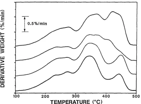
Typical thermogravimetric weight-loss and derivative weight-loss curves are shown in Fig. 1. It will be noted that several distinct regions are identifiable from both the weight-loss and its derivative curves. There is an initial weight- loss of about 5 % up to approximately 200~ which is assumed to be due to vola- tilization of water, fluids and lubricants. Between about 200 and 500~ the major weight-loss processes take place, and several weight-loss steps are de- cernable in the weight-loss curve and are more clearly identified in the deriva- tive weight-loss curve. These weight-loss steps can b e attributed to the degradation of the major polymers present in the ASR, along with other organic materials present which also degrade at these temperatures. Above 500~ al- though some polymer degradation may be occurring it was assumed that the weight-losses are associated with inorganic materials present in the ASR. For example the weight-loss occurring at about 640~ is probably due to the decar-

I-- "r" O ! LU 1 0 0 1.5 80 60- 40 r . m E 1.0 I-- -i- O 0 . 5 W N 0.0 ~ - 0 . 5 o 2bo 660 860 looo TEMPERATURE (~

Fig. 1 The weightqoss and derivative weight-loss curves for a typical ASR sample heated at 5 deg.min -1 in nitrogen

DAY et al.: PLASTIC WASTE STREAM 401

boxylation of calcium carbonate, a material widely used as a filler in a variety of plastic components found in automotive applications [10].

Because the ASR solid waste is such a heterogeneous material and the sam- pling protocol involved taking 1-2 tonne samples in order to obtain a repre- sentative sample, the big concern of the analyst resolves around this use of a 12+1 mg sample for analysis. In order to address this concern we have con- ducted a series of experiments at different levels of sampling.

Table I Sampling procedure, nomenclature and coding

Level Sample size Test number Code Example

Operations - 4 A, B, C, D, E C

Samples 1-2 Mg reduced . 4 1, 2, 3, 4 C3

to 50 kg

Specimens 50 kg 4 a, b, c, d C3b

lkg

Sub-specimens 10 g 4 i, ii, iii, iv C3b(ii)

12 mg

In order to address these different levels of sampling the reader is referred to Table 1 which explains the sampling protocol and nomenclature used in this study. It should be pointed out, however, that in this current study we did not evaluate all the samples from all operations because of the magnitude of the task. Instead we restricted our comparisons to one sample from each of four op- erations, and likewise only all 4 samples from one operation. It should also be noted that each 50 kg sample was broken down into more than 4 specimens, but only 4 of these specimens, which weighed about 1 kg each, were actually ho- mogenized for this study [7]. Likewise these 1 kg specimens were riffled to give the 10 g sub-specimens from which the 12 mg test samples were taken for the TG analysis.

Sub-specimen variability

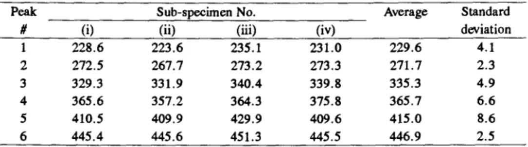
The derivative weight-loss curves for the four sub-specimens of ASR, C3b (i)-(iv) are presented in Fig. 2. Although the experiments were performed up to a final temperature of 950~ it was decided to only concentrate on the weight-loss up to 500~ since it was felt that it was this region that corre- sponded to the weight-losses associated with the polymeric materials. It must be noted that all four experiments displayed certain similar characteristics in terms of peak maxima positions along with certain similarities in peak shapes but are far from identical. Each curve was then individually subjected to the deconvo- lution program. The result of a typical deconvolution analysis are shown in

402 D A Y et al.: PLASTIC WASTE STREAM 0

F,,

Fig. 2 D e r i v a t i v e weight-loss curves for four sub-specimens o f A S R heated at 5 deg-min -I

in nitrogen r-. 1 . 5 , ~ ~ ... i ... ! ... ~ ... 1 . . . . ... i: ... ~ '... :/4' ... ";,f ... ~*" ... C.';"~'"t"\: "'": ... - - \ " it i E3 0.0 . . . . . . 1 0 0 2 0 0 3 0 0 4 0 0 5 0 0 T E M P E R A T U R E (~

Fig. 3 A typical deconvoluted derivative weight-loss curve showing the six de.convoluted peaks

DAY et al.: PLASTIC WASTE STREAM 403

Fig. 3. Each curve was deconvoluted into six individual peaks and each individ- ual peak was analyzed in terms of peak area and peak temperature maximum.

The results of this analysis are presented in Tables 2 and 3 for the peak tem- peratures and % areas, respectively. A similar analysis was performed on four other specimens from this sample i.e. specimens C3a, C3b, C3c and C3d and these results are summarized in Tables 4 and 5 for the peak temperatures and % areas, respectively. The data suggest that in terms of the position of the peak temperatures the variability from sub-specimen to sub-specimen is not very large with an average percent coefficient of variability of less than 2%. How- ever peak #1 showed the largest variability with an average coefficient of vari- ation of 4.1% with one set of sub-specimens showing a coefficient of variation of 8.1% with the peak temperature ranging from a low of 203.6~ to a high of 254.3~ However, even with this set of sub-specimens, the average for peak #1 at 227.5~ was very close to the average for the set of 229.7~ This same set of sub-specimens also showed a coefficient of variation of 4.3 % for the po- sition of peak #2 with values ranging from 267.7 to 289.8~ However once again the average peak value of 271.2~ was close to the average of 267.3~

Table 2 Peak temperature (~ for the sub-specimen samples C3b (i-iv)

Peak Sub-specimen No. Average Standard

# (i) (ii) (iii) (iv) deviation

1 228.6 223.6 235.1 231.0 229.6 4.1 2 272.5 267.7 273.2 273.3 271.7 2.3 3 329.3 331.9 340.4 339.8 335.3 4.9 4 365.6 357.2 364.3 375.8 365.7 6.6 5 410.5 409.9 429.9 409.6 415.0 8.6 6 445.4 445.6 451.3 445.5 446.9 2.5

Table 3 Peak areas (%) for the sub-specimen samples C3b (i-iv)

Peak Sub-specimen No. Average Standard

# (i) (ii) (iii) (iv) deviation

1 22.2 16.8 20.1 24.8 21.0 2.9 2 7.4 15.7 9.2 7.8 10.0 3.3 3 16.6 25.4 26.4 32.5 25.2 5.6 4 18.8 23.7 26.5 14.0 20.7 4.8 5 20.7 7.8 8.1 12.6 12.3 5.2 6 14.1 10.6 9.8 8,2 10.7 2.2

In general it was found that peaks #1, 3 and 4 represented the major con- tributors to the total area, on average accounting for 20, 25 and 25% of the total

4 0 4 D A Y et al.: P L A S T I C W A S T E S T R E A M I-I ..-t . " ~ ~ 9 ~ . ~ ~

I

~.~

~.~

DAY et al.: PLASTIC WASTE STREAM 405 U

~d

~.~

" ~ ~

4 0 6 D A Y et a l . : P L A S T I C W A S T E S T R E A M "?, 0 v o = .~. 2 ~

t ~

~~

D A Y et al.: P L A S T I C W A S T E S T R E A M 4 0 7 r ,-.. ,-'. r ,..., (4 ei o r ,,Q ",3 ~ 3". Thermal Anal., 42, 1994

408 DAY et al.: PLASTIC WASTE STREAM

area respectively. Meanwhile, peaks #2, 5 and 6 on average each contributed approximately 10%.

However, the sub-specimen variability was high with the smaller peaks #2, 5 and 6 showing the greatest average coefficients of variation of 32, 34 and 29 % respectively, with an individual sub-specimen set showing values as high as 54% (peak #5 specimen C3c). This type of variability in the peak area clearly reflects the problems of employing such small sample sizes to measure the com- position of such a heterogeneous material.

Specimen variability

In terms of specimen to specimen variability for one sample from one opera- tion, the results are summarized in Tables 4 and 5, for the peak temperatures and the % areas, respectively. The mean and standard deviation for the speci- mens were calculated in two ways. The first involved a standard calculation based upon the average value obtained for the sub-specimens. The second in- volved the calculation of the weighted mean [12] which takes into consideration the standard deviation obtained with the sub-specimens. The net effect of the weighted mean calculation was to give greater credence to the values with low standard deviations and lower credence to the values with high standard devia- tions. In terms of actual average peak temperatures and measured areas the cal- culated values using the two processes were very similar. However, in terms of the coefficient of variation large differences were noted depending upon the sta- tistical approach used. For example in the case of the peak temperature, em- ploying a weighted mean, the highest coefficient of variation was 1.4% observed for peak #1. However, when straight statistics were employed the highest coefficient of variation was obtained with peak #4 at 1.8 %.

When the peak areas are considered, larger coefficients of variation are evi- dent than were noted with the peak temperatures. The average value for the weighted mean statistics was 11.3%; with standard statistics giving a value of 15.2%. Once again, the largest variability was noted for the smaller peaks #2, 5 and 6 (i.e. 23.3, 25.8 and 2.7%) than for the larger peaks #1,3 and 4 (i.e. 11.2, 16.9 and 11.2%); peak #6 proving to be an exception. Comparing the sub-specimen to specimen variability it is clear that the averages of the sub- specimen data are responsible for an apparent improvement in the specimen variability as can be seen by comparing the numbers for the sub-specimen and specimens in Tables 4 and 5.

Sample variability

The results of the sample to sample variability measurements for the peak temperatures and peak areas are given in Tables 6 and 7, respectively. Once J. Thenna/ AnaL, 42, 1994

DAY et al.: PLASTIC WASTE STREAM 409

again the mean and standard deviation of the samples have been calculated in the standard statistical manner in addtion to the weighted mean and standard de- viation approach. It will be noted that once again the coefficients of variation are much lower for the peak temperatures than those observed with the peak ar- eas. However, the peak temperatures are beginning to show increased variabil- ity, especially peaks #1 and 2. For example with peak #1 coefficients of variation of 3.3% and 1.5% are noted using the standard and weighted statisti- cal approaches and the calculated mean values are 255.4 and 265.0~ respec- tively. Average individual values for the peak #1 were also noted to vary from a low of 245.7~ to a high of 268.80C; a sizable difference. In a similar manner peak #2 also shows a high degree of variability, with average values ranging from a low of 283.6~ to a high of 306.1~ Meanwhile peaks #3, 4, 5 and 6 were noted to have much lower levels of variability comparable to the specimen variability noted previously.

Interestingly, however, when the peak areas are considered peaks #1 and 2 show similar coefficients of variation to those for peak #3, 4, 5 and 6. How- ever, the degree of variability was once again dependent upon the statistical method of calculation. The average coefficient of variability for the six peaks calculated by the weighted mean method was about 8.3% whilst it was as high as 17.8% for the standard method of calculation. This high variability was par- ticularly evident with peak #4, which ranged from a low of 13.1% to a high of 26.5 % with a coefficient of variation of 23.3 % calculated by standard statistics. Despite the variability in the peak areas between the four samples, peaks #1, 3 and 4 were still the major peaks with peaks #2, 5 and 6 contributing less to the total area.

Variability between operations

On progressing to examine the variability of the peak temperatures and peak areas between the four operations (Tables 8 and 9), a pronounced increase in the coefficients of variation were noted, especially when the values were calcu- lated using the standard statistical method. For example the average coefficient of variation for the six peak temperatures was 3.0% while that for the peak ar- eas was 21.2%.

Once again the largest variations in peak temperatures were noted for peaks #1 and 2 which had coefficients of variation of 7.0% and 5.0%, respectively when calculated using standard statistics. This variability appears to be associ- ated with the identification of these two peaks #1 and #2. For example peak #1 was identified at 227.5~ for operation C while peak #1 for the other opera- tions was located at about 268~ Similarly peak #2 for operation C appears centred at 269.9~ very close to the temperature identified for peak #1 for the

410 DAY et al.: PLASTIC WASTE STREAM

o

d ~ d d d ~ ~ d ~ d

DAY et al.: PLASTIC WASTE STREAM 411

r

412 DAY ,~t al.: PLASTIC WAST~ S T I ~ A M O p., E ~ . ~ ~, 0 u O ~ ',O (",1 r J. Thermal Anal., 42, 1994

DAY et al.: PLASTIC WASTE STREAM 413

J

414 DAY et al.: PLASTIC WASTE STREAM 0 ~

~'~

.~ i

D A Y et al.: P L A S T I C W A S T E S T R E A M 415 o 0 i . ~ ~ o o o o cq P~ O~ rz ~4 ~- ,n: J. Thermal Anal., 42, 1994

416 D A Y et al.: PLASTIC W A S T E STREAM 0 0 e~ ,. el ~ ~ o 0 0 0 ~ 0 ~ 0 c'4 r j. Thermal Anal., 42, 1994

D A Y et a l . : P L A S T I C W A S T E S T R E A M 4 1 7 o ~ 0 o o o t"-I t"-I ~ ~ c4 o< r o< t"4 4 o o o o m u ~ m ~ m J. Thermal Anal., 42, 199,t

418 DAY et al.: PLASTIC WASTE STREAM

other'operations. Clearly this ambiguity iri the assignment of peaks #1 and 2 is a major concern and suggests that in the 200 to 300~ temperature region we could be dealing with more than just two components contributing to this weight-loss zone.

Meanwhile, in the case of peaks #3 to 6 the position of the peak temperature is relatively constant although the variability between operations is definitely greater than that observed for sample variability and specimen variability.

In terms of peak areas, once again, larger coefficients of variation are noted for the variability between operations than was observed with the samples and specimens. For example, average values for peak areas of 21.2% and 13.7% were obtained for the coefficients of variation by standard statistics and weighted statistics respectively. In fact some very high coefficients of variation were observed for individual peaks such as 35.1% for peak #6 and 27.3% for peak #1 when standard statistics were employed. This variability is clearly evi- dent with peak #6 which had an average area of only 8.7 % from operation D while that measured for operation E was 21.7%. Meanwhile the observed peak areas for peak #1 were 28.7% and 14.0% for operation D and E respectively.

Table 10 Summary of peak temperature (~ results

Peak Specimens Samples Operations

# Average Std. Dev. Average Std. Dev. Average Std. Dev.

1 229.7 3.0 255.4 8.4 258,7 18.1 2 269.3 2.8 294.4 8.6 295.4 14.8 3 335.1 1.2 350.5 2.0 343.5 6.3 4 375,6 6, 9 388.3 3.4 382.1 4.6 5 418.1 3.9 421.7 6.1 421.1 7.3 6 449.6 3.0 450.1 4.7 450,8 4.9

The results of this statistical analysis are summarized in Tables 10 and 11 for the peak temperatures and peak areas respectively using the standard statistical data. In the case of the peak temperatures it is clear that on progressing from specimen to sample to operation the degree of variability is increasing. This in- crease in variability is especially noticeable for peaks #1 and 2 where the as- signment of only two peaks to the degradation zone 200-300~ is questionable (Fig. 3). In terms of the weight-loss steps it appears that peaks #1, 3 and 4 are the major contributors, accounting for about 70% of the total while the other three peaks #2, 5 and 6 together only contribute approximately 30% to the to- tal. In terms of variability in peak areas there are large variations in all cases with only as light increase in the measured coefficients of variation on progress- ing from specimens to samples to operations.

DAY et al.: PLASTIC WASTE STREAM 419

Table 11 Summary of peak area (%) results

Peak Specimens Samples Operations

# Average Std. D e v . Average Std. D e v . Average Std. Dec.

1 19.6 2.2 16.3 1.4 20.4 5.6 2 12.9 3.0 10.5 1.3 8.6 1.0 3 24.9 4.2 35.5 6.9 20.0 3.5 4 22.3 2.5 21.0 4.9 25.9 3.5 5 9.3 2.4 6.2 1.5 9.6 2.1 6 11.0 0.3 10.5 2.0 13.9 4.9 P e a k i d e n t i f i c a t i o n

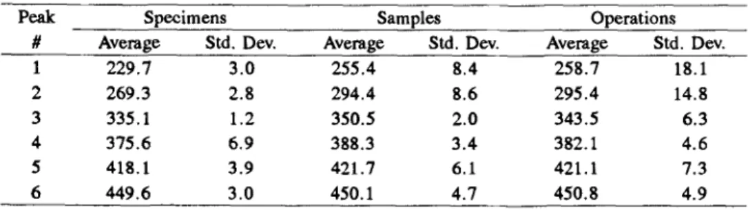
The derivative TG curves for some of the major polymers used in the auto industry are presented in Fig. 4. Also included in this figure are d e c o n v o l u t e d curves for an ASR sample.

Based u p o n an examination o f the information presented in Fig. 4, it be- c o m e s possible to speculate u p o n the p o l y m e r s responsible for the different

"r

1"7i

pp

uJ

n-

>-

ABS

LLI

P V C ~

1 O0

200

300

400

500

TEMPERATURE (~

Fig. 4 Comparison of the derivative weight-loss curves from PP, ABS, PU and PVC and a deconvoluted ASR sample

420 DAY et al.: PLASTIC WASTE STREAM

peaks observed in this ASR sample. For example the high temperature peak #6 in ASR at about 450~ could be attributed to PP with some possible contribu- tion by PVC. Peak #5 at about 420~ meanwhile may be attributed to ABS. Likewise peak #4 at about 380~ may be due to PU. Meanwhile PU and PVC could also contribute to peaks 2 and 3 at about 290 and 340~ respectively. Peak #1 at about 250~ however appears to be due to some other material which need not be polymeric such as engine oil, lubricants, etc.

However, in a previous study we have shown that binary mixtures of these polymers can result in interactions causing changes in peak temperatures [11]. In this earlier study we compared experimental and calculated information and noted that interactions occurred in the degradation of mixed polymeric compo- nents. The use of the deconvolution procedure described in this paper was therefore used to analyse a series of binary polymer mixtures in an attempt to assist the peak identification process. The results of these studies are summa- rized in Table 12.

Table 12 Peak temperature (~ for binary mixtures

Pure Experimental mixtes polymer 25/75 50/50 75/25 PP/ABS PP 449.9 447,0 449.8 452.6 ABS 411.8 402.9 404.8 405.3 PP/PVC PP 449.9 450.5 453.9 454.5 PVC 453.1 460.7 460.3 459,5 PVC 296.1 293.1 292.6 293.1 PP/PU PP 449.9 443.9 442.6 446.2 PU 374.9 375.6 391.9 410.9 PU 292.6 291.8 285.7 283.4 ABS/PVC ABS 411.8 403.9 404.2 406.7 PVC 453.1 447.6 434.0 441.3 PVC 296.1 288.7 286.0 284.4 ABS/PU ABS 411.8 403.9 408.2 407.3 PU 374.9 376.8 389.1 391.9 PU 292.6 292.7 289.8 285.4 PU/PVC PU 374.9 363.3 373.5 377.9 PU 292,6 274.7 282.8 288.8 PVC 453,1 455.2 451.5 453.6 PVC 296.1 282.4 278.7 271.6 J. Thermal Anal., 42, 1994

DAY et al.: PLASTIC WASTE STREAM 421

From this data it is clearly seen that when polymers are mixed interactions may occur causing the position of peak temperatures to shift. The extent of these temperature shifts, however, appear to be dependent upon the polymer mixtures and their concentrations.

In the case of the PP/ABS mixtures, little interactions appear to be taking place, i . e . the peak temperatures for both the PP and ABS are relatively inde- pendent of the composition of the mixture.

The PP/PVC mixtures meanwhile show some sort of interactions. However, because of the overlap of the two high temperature peaks some difficulty in peak temperature assignment is encountered. Essentially, however, the PVC ap- pears to be responsible for a shift in the peak temperature of PP to higher tem- peratures while the PP appears to be responsible for a similar slight shift in the higher PVC temperature peak. Meanwhile the lower PVC temperature peak is shifted to lower temperatures due to the presence of PP.

In the case of the PP/PU mixtures an increase in PU content in the mixture appears to cause the PP peak to shift to lower temperatures. Meanwhile the two PU peaks also shift due to the presence of the PP, but in opposite directions. The high temperature PU peak moves from 375.6 to 410.9~ as the concentra- tion of PP increases from 25 to 75%. Meanwhile, the same change in PP con- centration causes the lower PU peak to fall from 291.8 to 283.4~

In the case of the ABS/PVC mix, the PVC appears to be responsible for a reduction in the ABS peak temperature from 411.8~ for the pure polymer to 403.9~ for the 25/75 mixture. Meanwhile, as was noted with the PP/PVC mix- ture, the lower PVC peak temperature falls with increased ABS content. How- ever, contrarily to what was noted with the PP/PVC mixtures the high PVC peak temperature also falls with increasing ABS content.

The behaviour of the ABS/PU mixture mirrors that of the PP/PU mixtures. Increased PU content causes a fall in the ABS peak temperature from 411.8 to 403.9~ while the ABS caused the higher temperature PU peak to increase for 374.9 to 391.9~ while the lower temperature PU peak falls from 292.6 to 285.4~

In the case of the PU/PVC mixtures all peaks showed movement due to the presence of the other polymer with the exception of the higher temperature PVC peak which appears to be independent of mixture composition. In the case of both PU peaks, an increase in PVC content in the mixture resulted in a lowering of the PU peak temperatures. Meanwhile the lower PVC temperature peak shifted from 296.1 to 271.6~ as the concentration of PU was increased.

Based upon this information it is clear that peak assignment based upon the behaviour of the individual polymers is not a reliable prediction of peak tem- peratures when real mixed polymers are being considered.

422 DAY et al.: PLASTIC WASTE STREAM

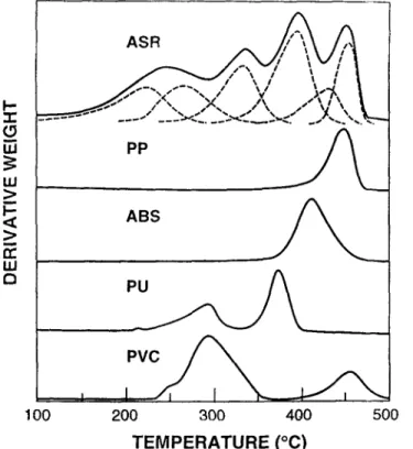
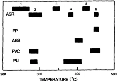
The assist the peak assignment of ASR samples the results of this binary mixture study have been summarized in Fig. 5. From this figure it would ap- pear that the peak temperatures associated with PVC and PU are the ones most strongly influenced by the presence of other polymers in binary mixtures. The PP and ABS peak temperatures are meanwhile influenced least by other poly- mers in that they both show narrow peak temperature ranges.

1 3 5 2 i 4 i 6

ASR

i

m

l

AB$

Fig. $ Peak temperature assignment for the six derivative weight-loss peaks in ASR and PP, ABS, PU and PVC

The information presented in Fig. 5 can now be used to assign the polymers to the various peaks identified in the ASR samples. For example it appears that peak #4 can be safely assigned to PU, the presence of which is easily recog- nized in ASR samples. Based upon this assignment and data from the analysis of several PU mixtures with other polymers in which it has been found that the area of the higher PU temperature peak contributes approximately three times that of the lower peak, the major part of peak #2 can also be assigned to PU. The consequence of this is that PVC can only contribute to a limited extent to peak #2. However, with PVC the peak area ratio between the lower and higher peaks is 2:1. This means that peak #6 cannot be assigned to PVC, but must be mainly due to the presence of PP. Some small PVC contribution cannot be ruled out but based upon chlorine analysis [13] is less than 3%.

It would therefore appear likely that in terms of polymeric composition, PU and PP are the major polymeric components present in the ASR samples with small contributions from PVC and ABS.

DAY r al.: PLASTIC WASTE STREAM 423 I--

<

h

TEMPERATURE (~

Fig. 6 C o m p a r i s o n o f a d c c o n v o l u t e d A S R s a m p l e and a synthetic p o l y m e r m i x c o m p o s e d o f P U ( 3 0 % ) , P P ( 4 5 % ) , F i b r e s ( 1 5 % ) and oil (10%)

In order to verify the logistics of this type of analysis a composite mix was prepared containing 30% PU and 45% PP to which was added 15% fibrous ma- terial (sound deadening material) taken from an old automobile and 10% engine oil. This composite was subjected to TG analysis and the deconvoluted deriva- tive curve is shown in Fig. 6 along with the deconvolution analysis of an ASR sample. It will be noted while the match is not positive the peaks do show some similarities. However, the added complications of metal contaminants such as rust, copper, etc. need to be taken into consideration [14].

C o n c l u s i o n s

The composition of ASR is a complex mixture of polymers contaminated with numerous materials. The organic composition shows a high degree of vari- ability between specimens, samples and operations. The use of TG coupled with a computer software program to convolute overlapping peaks obtained from the derivative weight-loss curves can be used to give some indication of the poly- J. Thermal Anal., 42, 1994

424 DAY r ai.: PLASTIC WASTE STREAM

meric composition of such a mixed plastic waste stream. However, because, of the small sample size and the large degree of heterogeneity of the waste, quan- titative interpretation of the data is extremely difficult. The technique may have some merit when dealing with a more homogeneous plastic waste stream such as that generated by a plastic recycling collection program. However, in order to obtain meaningful information it is essential to employ an acceptable sam- pling protocol along with the analytical technique to ensure that the repre- sentative samples being analyzed are worthy of analysis.

R e f e r e n c e s

1 T. Ratray, Resource Recycling, 5 (1993) 65.

2 T. R. Curlee and S. Das, Resources, Conservation and Recycling, 5 (1991) 343. 3 J. W. Everett and J. J. Peirce, Resource, Conservation and Recycling, 6 (1992) 355. 4 F. Rodriguez, L. M. Vane, J.-J. Schreiter and P. Clark, ACS Syrup. Series, 509 (1992) 99. 5 American Iron and Steel Institute. Special Report: "Recycling: State of the Art for Scrapped

Automobiles Rept. #67110, 1992.

6 Plastics Institute of America, Secondary Reclamation of Plastic Waste, PIA Research Report Phase I: Development of Techniques for Preparation and Formulation, Technomic Publish- hag, 1987.

7 M. Day, J. Graham, R. Laehmansingh and E. Chen, Resource Conservation and Recycling, 9 (1993) 255.

8 E. Nieto, "Technical Support Document for Treatment Levels for Auto Shredder Waste" Fi- nal Report, State of California Department of Health Services, 1989.

9 M. Day, SAE Technical Paper 93-0562 March 1993. 10 S. J. Ainsworth, Chemical and Eng. News, 70 (1992) 34.

11 M. Day, J. D. Cooney and C. Klein, J. Thermal Anal., 40 (1993) 669.

12 R. J. Cvetanovie, D. L. Singleton and G. Paraskevopoulos, J. Phys. Chem., 83 (1979) 50. 13 V. Boyko, (Private Communications) 1993.

14 M. Day, J. D. Cooney and M. MacKinnon, "Recycling Mixed Plastic Waste Streams: I1 The role of impurities on Pyrolysis Processes" Proc. 22nd NATAS Conference, Sept. 1993, p. 556.

Z u s a m m e n f a s s u n g - Die Thermogravimetrie gemischter Polymerabfallstrrme wurde unter- sueht und das Gewichtsverlustverhalten dieser heterogenen Gemische mit den Resultaten der Ge- wichtsverlustkurven einiger reiner Polymere verglichen. Die Ergebnisse weisen darauf hin, dab das Verhalten des Gemisches nieht anhand eines einfachen additiven Verhaltens der Polymer- komponenten vorausgesagt werden kann, da Wechselwirkungen auftrcten krnnen, wclche die Gewiehtsverlustprofile der Zersetzungen bceinflussen. Der untersuehte hetemgene Polymerabfall wurde dutch Zerldeinerung yon alten ausrangierten Automobilen gewonnen. Die Resultate der Untersuchung zeigen, dab es mrglich ist, zu bestimmen, was in einer Probe enthalten ist, dab jedoch die Relevanz der Daten bei einem sehr heterogenen Abfallstrom fraglich ist.