HAL Id: hal-01393361
https://hal.inria.fr/hal-01393361v2
Submitted on 31 Jan 2017
HAL is a multi-disciplinary open access
archive for the deposit and dissemination of
sci-entific research documents, whether they are
pub-lished or not. The documents may come from
teaching and research institutions in France or
abroad, or from public or private research centers.
L’archive ouverte pluridisciplinaire HAL, est
destinée au dépôt et à la diffusion de documents
scientifiques de niveau recherche, publiés ou non,
émanant des établissements d’enseignement et de
recherche français ou étrangers, des laboratoires
publics ou privés.
Spatio-Temporal Predictability of Cellular Data Traffic
Guangshuo Chen, Sahar Hoteit, Aline Carneiro Viana, Marco Fiore, Carlos
Sarraute
To cite this version:
Guangshuo Chen, Sahar Hoteit, Aline Carneiro Viana, Marco Fiore, Carlos Sarraute. Spatio-Temporal
Predictability of Cellular Data Traffic. [Research Report] RT-0483, INRIA Saclay - Ile-de-France.
2017, pp.17. �hal-01393361v2�
ISSN 0249-0803 ISRN INRIA/R T --483--FR+ENG
TECHNICAL
REPORT
N° 483
November 2016 Project-Teams INFINEPredictability of Cellular
Data Traffic
Guangshuo Chen, Sahar Hoteit, Aline Carneiro Viana, Marco Fiore,
Carlos Sarraute
RESEARCH CENTRE SACLAY – ÎLE-DE-FRANCE 1 rue Honoré d’Estienne d’Orves Bâtiment Alan Turing
Campus de l’École Polytechnique 91120 Palaiseau
Guangshuo Chen
∗†, Sahar Hoteit
‡, Aline Carneiro Viana
†,
Marco Fiore§, Carlos Sarraute
¶Project-Teams INFINE
Technical Report n° 483 — November 2016 — 19 pages
Abstract: The knowledge of the upper bounds of mobile data traffic predictors provides not
only valuable insights on human behavior but also new opportunities to reshape mobile network management and services as well as provides researchers with insights into the design of effective prediction algorithms. In this paper, we leverage two large-scale real-world datasets collected by a major mobile carrier in a Latin American country to investigate the limits of predictability of cellular data traffic demands generated by individual users. Using information theory tools, we measure the maximum predictability that any algorithm has potential to achieve. We first focus on the predictability of mobile traffic consumption patterns in isolation. Our results show that it is theoretically possible to anticipate the individual demand with a typical accuracy of 85% and reveal that this percentage is consistent across all user types. Despite the heterogeneity of users, we also find no significant variability in predictability when considering demographic factors or different mobility or mobile service usage. Then, we analyze the joint predictability of the traffic demands and mobility patterns. We find that the two dimensions are correlated, which improves the predictability upper bound to 90% on average.
Key-words: user profiling and personalization
This work was supported by the EU FP7 ERANET program under grant CHIST-ERA-2012 MACACO.
∗Université Paris Saclay, France †INRIA Saclay, France
‡Ecole d’ingénieurs du numérique ISEP, France §CNR - IEIIT, Italy
Prévisibilité spatio-temporelle du trafic de données
cellulaires
Résumé : La capacité de prévoir l’activité des abonnés par rapport à leur trafic de données
ouvre des nouvelles possibilités de remodeler la gestion et les services de réseaux mobiles. Dans cet article, nous exploitons deux grands ensembles de données réels collectés par un important opérateur mobile au Mexique afin d’étudier la prévisibilité des demandes de trafic de données cel-lulaires générées par les utilisateurs, de manière individuelle. Nous nous concentrons d’abord sur la prévisibilité des modèles de consommation de trafic mobile isolément. Nos résultats montrent qu’il est possible d’anticiper la demande individuelle avec une précision typique de 85%, et de révéler que ce pourcentage est cohérent pour tous les types d’utilisateurs. Malgré l’hétérogénéité des demandes des utilisateurs, nous constatons également une absence de variabilité significa-tive de la prévisibilité en tenant compte des facteurs démographiques, de la mobilité, ou de l’utilisation des services mobiles. Ensuite, nous analysons la prévisibilité des demandes de trafic combinée à des modèles de mobilité. Nous constatons que les deux dimensions sont corrélées, ce qui améliore la limite supérieure de prévisibilité à 90% en moyenne.
1
Introduction
The quantitative understanding of human behavior (e.g., a user’s whereabouts or data traffic) has recently emerged as a central question in multi-disciplinary research [1, 2, 3, 4, 5, 6, 7, 8, 9]. Individual actions cause dynamics that impact technological and economic phenomena of interest to many research communities. In wireless networking, the ability to foresee human activities has important implications in network design, management, control, and optimization [6, 7, 8, 9]. Specially, the better understanding of mobile data traffic consumption can help to improve the design of solutions for network load balancing, aiming at improving the quality of Internet-based mobile services. Over the past decade, a considerable amount of literature has investigated on predicting Internet traffic, such as [10, 11, 5].
The performance of any practical technique that aims at anticipating human behaviors is bounded by its predictability, which evaluates to what degree a specific behavior can be foreseen. The knowledge of the upper bounds of mobile data traffic predictors not only provides valuable insights on human behavior, but also opens new opportunities to network operators to manage their resources in advance, so as to accommodate the future demand at lower maintenance and operational costs. Besides, studies on per-user traffic consumption predictability allows defining traffic plans that are better tailored to users’ needs. Finally, understanding such upper bounds also empowers networking or service designers with the required knowledge to better deal with any constraints such bounds imply, as well as provides researchers with insights into the design of effective prediction algorithms.
The interplay between the regularity and the randomness determines the predictability. For instance, the temporal order of a user’s visited locations limits the predictability of her mobil-ity [4]; the statistical characteristics such as long-range dependence [12] and self-similarmobil-ity [13] restricts the predictability of Internet traffic in wired networks [14] or in cellular base sta-tions [10, 11]. In particular, for mobile phone subscribers, the regularity of their Internet traffic is not only reflected by the statistics of data [15, 16, 17] but also related to the user’s where-abouts [18]. However, at the best of our knowledge, there is no analysis of (i) how per-user regularity of mobile data traffic is translated into actual predictability, or (ii) the associated impacts brought by users’ visited locations.
In this paper, we aim at filling the gap above, and provide a first investigation of the pre-dictability of mobile data traffic generated by individual users. Specifically, we focus on data traffic volume, i.e., the amount of bytes generated by the mobile services consumed by a given subscriber. Overall, our study allows answering an important question: to what degree is the individual consumption of mobile data traffic predictable?
We address this problem by studying the variation in individual’s mobile data traffic over
timeand space and by investigating its predictability limits. To that end, we mine two large-scale
real-world datasets describing the cellular communication activity of thousands of subscribers, and leverage tools from information theory to determine predictability bounds. Our approach let us derive promising upper bounds to the performance of practical algorithms for the prediction of the volume of mobile data traffic generated by each user.
Our contributions are summarized as follows:
• We provide a first study of the predictability of mobile data traffic usage from the viewpoint of individual subscribers. We derive a promising upper bound (i.e., 85% on average) to the performance of practical algorithms for the prediction of the volume of mobile data traffic generated by each user by just considering temporal correlations in the traffic.
• We prove the result above to hold across heterogeneous classes of subscribers, based on age, gender, mobility, or mobile service usage.
• We extend the methodology so as to account for the joint predictability of single users’ traffic consumption and movement patterns. This let us investigate whether it is possible to forecast when, where, and how much mobile data traffic is generated by individual subscribers.
• We observe a 90% potential predictability of the spatio-temporal data consumption patterns of individual users. This result is due to the strong correlation between mobility and mobile
4 Guangshuo Chen, Sahar Hoteit, Aline Carneiro Viana, Marco Fiore, Carlos Sarraute service usage, i.e., to the fact that subscribers tend to generate similar amounts of traffic at each location. This suggests the feasability of anticipating how much mobile data traffic (as an order of magnitude) will be consumed by a given subscriber and where this will occur in a very effective manner, by knowing the past history of activities of the target individual. Although spatio-temporal information of subscribers can further improve the design of prediction model, we also find that the gain is not dramatic with respect to a technique that only relies on temporal information (i.e., 85%).
The rest of the paper is organized as follows. Sec. 2 sheds light on the related works from the literature. In Sec. 3, we introduce the concept of predictability and the methodology to compute it. In Sec. 4, we present our datasets and discuss data preprocessing. Sec. 5 discusses the pre-dictability of mobile data traffic in isolation. Sec. 6 extends the analysis to the joint prepre-dictability of mobility and data traffic. Sec. 7 discusses the cause of the high (joint) predictability and sheds light on the design of predicting algorithms. Finally, Sec. 8 concludes the paper.
2
Related work
Since the turn of the millennium, traffic predictability has attracted attention in the wired net-working community [14, 19]. As a consequence, the literature on the study of cellular network traffic has grown dramatically [1]. A number of studies have attempted to understand cellular data traffic. The authors in [16] modeled the volume distribution of Internet data traffic towards an improved traffic volume prediction. Oliveira et al. [17] proposed a measurement-driven model of mobile data traffic and a synthetic mobile data traffic generator. Both these studies do not consider the influence of subscribers’ mobility on their mobile service consumption. The relation between content consumption and mobility properties is considered in studies that focus on ap-plication interests [20], data traffic dynamics [15] and service usages [18]. However, none of these works provides a complete analysis of the predictability of the mobile data traffic consumption of individual subscribers, with respect to both time and space dimensions – as done in this work. Recently, two studies contributed to our understanding of the predictability of cellular data traffic. Zhou et al. [10] analyzed the predictability of voice, text, and data traffic in cellular networks. Li et al. [11] focused on the traffic predictability in Cloud radio access networks (C-RANs) and proposed future potential of software-defined C-RAN paradigms that benefit from the traffic prediction. These two works have an aggregated perspective, only distinguishing all traffic served by each base station. Instead, we analyze the traffic predictability from the viewpoint of individual users, as motivated in the introduction.
Our analysis is driven by information theory [21]. Tools of entropy estimation are introduced in [22], including the entropy estimator we used in the paper. Entropy is a concept found in many studies investigating spatial or temporal characteristics of cellular network data [23, 16, 20]. Our work is mainly based on the research of Song et al. who were the first to use information theory to investigate the predictability of human mobility [4, 24]. However, the goal of our study is different, as the target is mobile data traffic volume predictability, studied in isolation as well as jointly with mobility.
3
Measuring predictability
In this section, we define the concept of predictability as employed in our work, and show how its upper limit can be derived from entropy. Our methodology follows that first proposed in [4], which has been successfully employed to investigate the predictability of human mobility [4, 25], mobile data traffic [10], and vehicular traffic [26]. We favor the definition of predictability in [4] over equivalent ones (e.g., those in [27] and [14]), since it is more easily adapted to the study of the joint predictability of mobility and mobile data traffic demands, which is our ultimate objective.
3.1
Predictability
Consider a particular human behavior (e.g., a user’s whereabouts or data traffic volumes), which could be discretized and be measured regularly at every time interval. Its predictability at the
ith time interval, denoted as Π
i, is defined as the maximum probability of correctly forecasting
the current state from a known set of possible outcomes. Leveraging the concept of expected
value, the overall predictability is then defined as: Π ≡ limT →∞ T1 P
T i=1Πi.
As indicated in Sec. 1, we are interested in investigating the predictability of the volume of data traffic generated by mobile phone subscribers, in isolation as well as jointly with the geographical locations where they consume the associated mobile services. The computation of the overall predictability requires knowledge of the expected predictability over an infinite time interval. Since measurement periods are finite in any practical setting, we model user-generated data traffic demands and user movements as stochastic processes. We then compute an upper bound on each of their predictability. To that end, we employ the empirical estimation proposed in [4] and its supplement [24], presented next.
3.2
An entropy-based upper bound of predictability
In information theory [21], entropy measures the degree of uncertainty or disorder of an informa-tion flow. Intuitively, entropy and predictability are negatively correlated variables: a random process with low (or high) uncertainty is highly (or little) predictable. Song et al. [4, 24] studied this correlation for human mobility analysis and established an explicit formula from the
intu-ition. Their formula quantifies the correlation between entropy H(X) (or entropy rate Hu(X))
and an upper bound on predictability Πmax
u , and is summarized as follows.
Recall the human behavior mentioned above. Let discrete random variable Xi denotes the
discretized behavior at the ithtime interval with probability mass function p
i(x) = Pr(Xi= x).
Its entropy is formulated as H(Xi)≡ −Pxi∈Xipi(xi) log2pi(xi)[21]. Its predictability, denoted as Πi, is linked with its entropy by the inequality as H(Xi)≤ HF(Πi, Ni)where Niis the number
of possible states at the ith time interval and H
F(p, N ) is a function defined as: HF(p, N ) =
p log2p + (1− p) log2N −11−p. Because HF(p, N )is monotonically increasing, the upper bound of Πi
is derived from the inequality as Πi ≤ Πmaxi where Πmaxi satisfies H(Xi) = HF(Πmaxi , Ni). We
could calculate an upper bound of any human behavior’s predictability if we knew its entropy
at the ith interval. According to [24], this upper bound estimation is tight: It could be possibly
achieved by an actual algorithm.
Consider a time series of behaviors, denoted as X = {X1,· · · , XT}. Similarly, its entropy rate
is defined, regarding to the joint entropy of all behaviors over T time intervals in X, as follows:
Hu(X) ≡ lim T →∞ 1 T T X i=1 H(Xi|Xi−1,· · · , X1). (1)
It could be regarded as per-symbol entropy describing the mean degree of uncertainty of each behavior given the condition of being aware of past ones. As a bridge between its entropy rate
and its overall predictability, the following inequality stands: Hu(X) ≤ HF(Π, N ) where N is
the number of all possible states which may appear in the time series. From this inequality, an
upper limit of the overall predictability is also derived as Π ≤ Πmax
u . Apparently, the upper
bound Πmax
u is the exclusive solution of the equation HF(Πmaxu , N ) =Hu(X).
In our work, human behaviors are analyzed on per-user basis. Thus, given a particular
behavior of a user u, we collect a time series of the studied behavior as Su, and calculate its
entropy rate and upper limit of the overall predictability. Because Su is a limited set and
consequently, is unsuitable to apply Eqn. 1, the entropy rate is empirically estimated on the Lempel-Ziv encoding [28] as: Hu(X) ˆ=Hestu (Su)≡ PT logT 2T
i=1Li, where T is the total number of time
intervals and Li is the length of the shortest subsequence beginning from i which never appears
before the ith interval. Theoretically, Hest
u (Su) converges to Hu(X) with T → ∞ [28]. For
the overall predictability, we calculate its upper bound by applying a numerical solver on the
corresponding equation. The solver receives N and Hu(X) as inputs and produces the upper
6 Guangshuo Chen, Sahar Hoteit, Aline Carneiro Viana, Marco Fiore, Carlos Sarraute
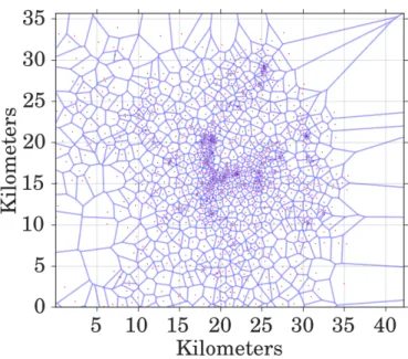
Figure 1: Deployment of cell towers in the observing area
4
Data overview
Our study is based on two real-world datasets describing the cellular network activity of hundreds of thousands of mobile phone subscribers (identically called users) of a major cellular operator in a metropolitan area. All data refer to a consecutive period of 92 days. The first dataset consists of call detail records (CDRs) containing timestamped and geo-referenced logs (i.e., of the closest mobile cell tower) of each voice call performed by every user. The second dataset describes the
Internet data sessions established every time a mobile device needs to exchange IP data traffic
through the cellular network.
These two datasets provide different and complementary information: CDR data includes location information that allows reconstructing user mobility, while session data only presents the mobile data traffic volume generated by each subscriber (with no associated geo-referenced log). In both cases, we preprocess the datasets to construct time series of subscriber’s locations and data traffic demands that are representative and statistically significant.
4.1
Datasets
CDR dataset: Call detail records are logged every time a mobile device makes or receives a
voice call. Each entry contains the hashed identifiers of the caller and callee, the call duration in seconds, the timestamp of the call start time and the location (latitude and longitude) of the cell tower to which the device is connected when initiating the phone call.
From a spatial perspective, cell tower locations are fairly dense in the center observing area, as shown in Fig. 1, where (red) dots represent the base stations and the Voronoi tessellation
approximates the coverage of each cell: on average, a cell tower covers a 2 km2area. This grants
a fair granularity in the localization of mobile subscribers. From a temporal perspective, the frequency of CDR entries (i.e., of phone calls) is not uniform over time. We observe that users are more keen to make or receive calls during daytime than nighttime.
Internet data session dataset: Every Internet data session is established upon the allocation
of a radio channel for the exchange of IP traffic, and it ends after an idle period over the same channel. Each entry in the dataset contains the hashed device identifier. The same hashing function is used in the CDR and Internet data session datasets, which allows linking users in the two datasets. The volume of upload and download data exchanged in KiloBytes, and the timestamp denoting the starting time of the session.
The dataset does not contain spatial information, but, from a temporal perspective, data sessions have a relatively uniform pattern. This is quite different from voice calls and is mostly
100 101 102 103 104 105 106 107 Mobile data traffic per user (KB) 0.0 0.2 0.4 0.6 0.8 1.0 F (x ) CDF All Users Selected Users
(a) Mobile data traffic per user
102 103 104 105 106 Volume in an hour (KB) 0.0 0.2 0.4 0.6 0.8 1.0 F (x ) CDF All users Selected users 0 20 40 60 80 100 0.0 0.2 0.4 0.6 0.8 1.0 F (x )
(b) Mobile data traffic per hour
10 20 30 40 50 60 70 80 Age 0.000 0.005 0.010 0.015 0.020 0.025 0.030 0.035 P (x ) PDF
All Users (Men) Selected Users (Men) All Users (Women) Selected Users (Women)
(c) Age and gender
10−1 100 101 102 103
Distance (in KM) between real and estimated user’s positions 0.65 0.70 0.75 0.80 0.85 0.90 0.95 1.00 F (x ) CDF Stop-by-spothome Baseline (d) Validation of CDR enhancement
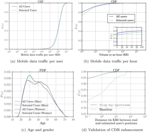
Figure 2: CDF of (a) the data traffic volume generated per user, (b) the data traffic volume generated per hour, and (c) the age categorized by the user’s gender over all mobile phone subscribers (solid blue curve) and the selected 45, 832 users (dashed green curve). (d) CDF of the spatial error (in km) between samples from the GPS and enhanced CDR data by the
stop-by-spothomeacross 84 users on the validation dataset.
due to automatically-generated background traffic and push notifications that are periodic and fairly independent of human activity.
To give a general overview of the mobile data traffic generated by the Internet session dataset, we plot the cumulative distribution function (CDF) of the total traffic volume generated by each subscriber in Fig. 2(a) and the traffic volume per subscriber on an hourly basis in Fig. 2(b), respectively. We remark that: (i) the data traffic generated by a subscriber is on average of 1.6 GB during the whole observing period, and significantly varies from 452 KB to 32GB; (ii) in
68% of hours, a subscriber does not start any new data session; (iii) the hourly traffic is highly
heterogeneous, and varies from 1 KB to 4.6 GB; (iv) only 6% of hours present a traffic volume higher than 1 MB/h. Besides, Fig. 2(c) portrays the distribution of the user’s age, showing that our datasets have almost all ages covered.
4.2
Data preprocessing
As detailed in Sec. 3, the calculation of the entropy rate and the corresponding upper bound on predictability requires discretized versions of the movements and demands of mobile phone subscribers. To this end, we proceed as follows. Firstly, we enhance the existing CDR dataset by adding the number of locations identified during nighttime, in order to enrich the mobility information captured by CDRs. Secondly, we filter subscribers in the datasets so as to ensure that their mobile activities allow accurate entropy estimation. Finally, using the selected subscribers
in each dataset, we compute representative discretized time series of locations Sloc
u and of data
traffic volumes Svol
u per user.
Enhancing CDR data: It is well-known that the events logged in CDR data tend to be
8 Guangshuo Chen, Sahar Hoteit, Aline Carneiro Viana, Marco Fiore, Carlos Sarraute a comparatively small number of measurements of location during nighttime as the source of mobility. In order to enhance the sparse CDR data and therefore improve the accuracy of the user location information, we employ the recent stop-by-spothome completion technique [29] which allows increasing the temporal coverage of CDR by adding more measurements between evening and morning without affecting the localization precision.
This stop-by-spothome technique infers a user’s home location and a period when a user stays at home. Formally, for each subscriber u ∈ U, where U is the observed population, it performs the following operations.
• The position of user u is considered to be the same associated to a CDR data entry (i.e., when a voice or sms event is triggered) 30 minutes before to 30 minutes after the entry timestamp.
• If two CDR entries are at less than 1 hour distance, then the transition from the location associated to the first entry and that associated to the second entry occurs (instantaneously) halfway between the two CDR entry timestamps.
• Considering the 3-month period of the dataset, the home location `H
u is determined as
the cell where u is most frequently found during the night time interval tH = (22h, 9h),
according to the CDR data.
• The home boundary time tH
u ⊆ tH is then defined as the most probable interval during
which the subscriber is found at `H
u in the CDR data.
• If a subscriber u’s location at a time instant t ∈ tH
u is unknown and if he was last seen at
no more than 1 km from this home location `H
u, he is considered to be at `Hu at time t.
We demonstrate the quality of the stop-by-spothome approach on a small dataset of users for which ground-truth data is available. We leverage the GPS trajectories of 84 users, sampled at a 5-minute frequency during a period ranging from a few weeks to several months, depending on the user. We subsample the GPS trajectory of each user, according to the empirical distribution of interarrivals of phone call events in the CDR dataset: this lets us recreate artificial CDR data from the complete GPS trajectories. Then, we apply the stop-by-spothome technique on the subsampled data, and compute the distance between the positions which are estimated by the stop-by-spothome and those in the ground-truth GPS trajectories. For the sake of completeness, we compare the result to that of a baseline approach that assumes users to remain static at the last observed location in between phone call events. Fig. 1(c) shows the excellent precision of stop-by-spothome with an error of 100 meters or less in 95% of cases, and much improved performance with respect to the baseline solution.
User filtering: To ensure statistical significance of the analysis, subscribers need to be
suffi-ciently active during the period under study to be tracked effisuffi-ciently via CDRs. For that and using the CDR dataset, we compute the incompleteness q for each subscriber, i.e., the fraction of hours during which no positioning information is available from the CDR entries. We then filter out subscribers with q ≥ 0.8 or who only visited 2 locations at most during the measurement period. These thresholds select users whose mobility information allows an accurate estimation of the location entropy [4, 24]. A total of 90, 726 users in our CDR dataset satisfy the conditions above.
In terms of data traffic, those users who do not generate traffic are not interesting for our study. Hence, we only consider users who actually leverage the cellular network for Internet access. To this end and using the Internet data session dataset, we calculate the daily volume of mobile data traffic generated by each subscriber in the Internet session dataset, and retain subscribers who establish sessions in at least 73 days (i.e., 80% of the observing period). As a result of our filtering process, 45, 832 subscribers are retained for our analysis.
A legitimate question is whether our filters introduce biases in the analysis. As shown in CDFs of Fig. 2(a) and Fig. 2(b), the distribution of mobile data traffic per user and per hour is consistent with that of the complete user set. In addition, as shown in Fig. 2(c), the selected users subset follows the same distribution of the user’s age and gender as the whole user population. Despite a minor bias in the fraction of hours during which no session is established, results show there is no bias introduced by the performed user filtering, since selected user subset is
still characterized by a strong heterogeneity in terms of ages, gender, and long-term demand of mobile data traffic (i.e., from light to heavy hitter users).
Volume integration: Leveraging the preprocessed data, we construct discretized time series of
the mobile data traffic generated by a subscriber u ∈ U as: Svol
u ={v1u, v2u, . . . , viu, . . . , vuT}, where
vi
u is a measure of the traffic volume generated by the subscriber u during the ithtime interval.
We consider four different temporal resolutions for time intervals: 15, 30, 45, or 60 minutes. In each case, we aggregate the volume of traffic from all sessions recorded during the corresponding interval. For instance, when the resolution is 60 minutes, the measurement period is divided into
T = 24 hours/day × 92 days = 2208 intervals, and the mobile data traffic is computed on an
hourly basis: This will be our default setting, unless stated otherwise.
As seen in Fig. 2(b), the hourly traffic volume varies across a wide spectrum, from KB/h
to GB/h. Since the traffic volume needs to be quantized in the Svol
u representation, we favor a
representation that captures the traffic magnitude over a uniform discretization. The rationale is that one is more interested in predicting whether a user will generate, i.e., KiloBytes, MegaBytes or GigaBytes of traffic, rather than if a user’s demand will be in the first (1 KB, 333 MB), second (334 MB, 666 MB) or third (667 MB, 1 GB) portions of one GB. Specifically, we employ the following five different quantizations of the traffic volume spectrum, listed in order of increasing accuracy:
• Q1: four quantization levels, i.e., idle (0 KB), light (1 KB, 1 MB), heavy (1 MB, 1 GB), and extremely heavy (1 GB, 10 GB).
• Q2: eight quantization levels, i.e., 0, (1, 10), (10, 102), . . . , (106, 107), all values in KB.
Once stated otherwise, Q2 will be our default setting.
• Q3: twelve quantization levels, obtained by bisecting each level over 1 MB in Q2, e.g., splitting (1,10) MB into (1,5.5) MB and (5.5,10) MB.
• Q4: sixteen quantization levels, obtained by trisecting each level over 1 MB in Q2. • Q5: forty quantization levels, obtained by nine-secting each level over 1 MB in Q2.
Location integration: The movement of a user u ∈ U is represented as a discretized time series
of locations, as follows: Sloc
u = {`1u, `2u, . . . , `iu, . . . , `Tu}, where `iu is the location of u in the ith
time interval spanning (ti
s, tie). The location is that of the main cell to which user u is attached
during time period (ti
s, tie). If that location is unidentified, i.e., no entry is available in the CDR
dataset for u during (ti
s, tie), `iu is marked as unknown. Since the CDR logs are sparse in time,
we only implement the temporal resolution of 60 minutes for time intervals. For that, the same measurement period as that of mobile data traffic is split into the T = 24 hours/day × 92 days =
2208hour-long intervals and each representative location is selected on an hourly basis.
5
Predictability of mobile data traffic
In this section, we study the predictability of the mobile data traffic generated by individual subscribers. For now, we focus on the forecast of traffic volume in isolation, and we will consider the joint predictability of traffic and mobility later on.
5.1
Methodology
We implement the method presented in Sec. 3 to empirically derive an upper bound on the
pre-dictability through the entropy rate. Formally, we consider a stochastic process V = {V1,· · · , VT}
that describes the mobile demand of a generic subscriber as a sequence of discretized traffic
vol-umes Vi, for each time interval i.
The actual entropy rate, denoted by Hu(V), depends no t only on the frequency of appearance
of each discretized traffic volume but also on the order in which they appear, capturing the
temporal order presented in a subscriber’s traffic usage pattern. Formally, Hu(V) is defined in
Eqn. 1 and models the process as a stationary stochastic process. For each user, an empirical
10 Guangshuo Chen, Sahar Hoteit, Aline Carneiro Viana, Marco Fiore, Carlos Sarraute
(a) Example: rapid entropy convergence
0.0 0.5 1.0 1.5 2.0 2.5 3.0 3.5 Entropy H 0.0 0.5 1.0 1.5 2.0 2.5 P (H ) PDF Hrand u (V ) Hunc u (V ) Hn0 u(V ) Hu(V) (b) Entropy 0.0 0.2 0.4 0.6 0.8 1.0
Upper limit of predictablity Π 0 1 2 3 4 5 6 7 8 9 P (Π) PDF Πrand u (V ) Πunc u (V ) Πn0 u(V ) Πmax u (V) (c) Predictability
Figure 3: (a) An example of the fast convergence: for three representative users: the entropy rate
converges rapidly to Hu(V) as Svolu includes an increasing number of days. (b) Distributions of the
random entropy Hrand
u (V ), the temporal-uncorrelated entropy Huunc(V ), the
nonzero-temporal-uncorrelated entropy Hn0
u (V ), and the entropy rate Hu(V) as observed in the individual traffic
demand generated by the selected 45, 832 users. (c) Equivalent distributions of the upper bounds
on the predictability Πrand
u (V ), Πuncu (V ), Πn0u (V )and Πmaxu (V).
converge rapidly enough (within a few days in our three-month data) in the case of practical traffic volumes. For this, we show in Fig. 3(a) an example of three typical users.
We leverage Svol
u to derive three additional variants of the entropy rate, which we will use to
investigate the properties of the process. The variants are as follows:
• The random entropy is computed by considering that each Viis equally probable and
time-independent in the process. The random entropy is Hrand
u (V ) ≡ log2N, where N is the
number of distinct quantizations of traffic volumes associated to a subscriber. It indicates
the theoretical maximum value of the entropy rate Hu(V).
• The temporal-uncorrelated entropy is formulated as Hunc
u (V ) ≡ −
P
v∈V p(v) log2p(v),
where p(v) is derived from Svol
u and represents the historical probability of a subscriber
to generate volume v, characterizing the heterogeneity of traffic demand patterns. The temporal-uncorrelated entropy characterizes a mobile demand process that has no tempo-ral correlations, hence its name.
• The nonzero-temporal-uncorrelated entropy is based on the same model of Hunc
u (V ),
but it is limited to those cases when the user is not idle. Formally, it is Hn0
u (V ) ≡
−P
v∈V /{0}p(v|v 6= 0) log2p(v|v 6= 0). The nonzero-temporal-uncorrelated entropy
cap-tures the heterogeneity of the traffic volume exchanged during active sessions only, assuming again that no temporal correlations exist among them.
It is worth noting that, naturally, for each subscriber: Hu(V) ≤ Huunc(V )≤ Hurand(V ).
As discussed in Sec. 3, an upper bound on the predictability can be computed from the entropy rate. In our context, this bound is an estimation of the maximum achievable accuracy in the prediction of the mobile traffic demand, given a particular model of the distribution of V.
Hence, four upper bounds for the predictability, indicated as Πrand
u (V ), Πuncu (V ), Πn0u (V ), and
Πmaxu (V), can be calculated from the entropy rates above.
In addition, recall that multiple representations of Svol
u are possible, depending on the
combi-nation of time granularity and volume quantization. For each such combicombi-nation, different results are obtained in terms of entropy rate and thus, predictability.
5.2
Baseline results
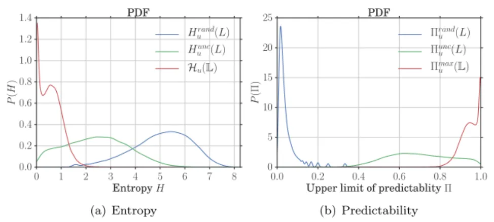
Our baseline results are shown in Fig. 3, and are obtained under 1-hour (time) and Q2 (traffic volume) quantization level described in Sec. 4.2. Specifically, Fig. 3(b) displays the probability
density function (PDF)1 of the four versions of the entropy rate presented in Sec. 5.1. Fig. 3(c)
portrays the PDF of the corresponding upper bounds on predictability.
1All PDFs are represented using kernel density estimation (KDE).
Q1 Q2 Q3 Q4 Q5 Data volume quantification
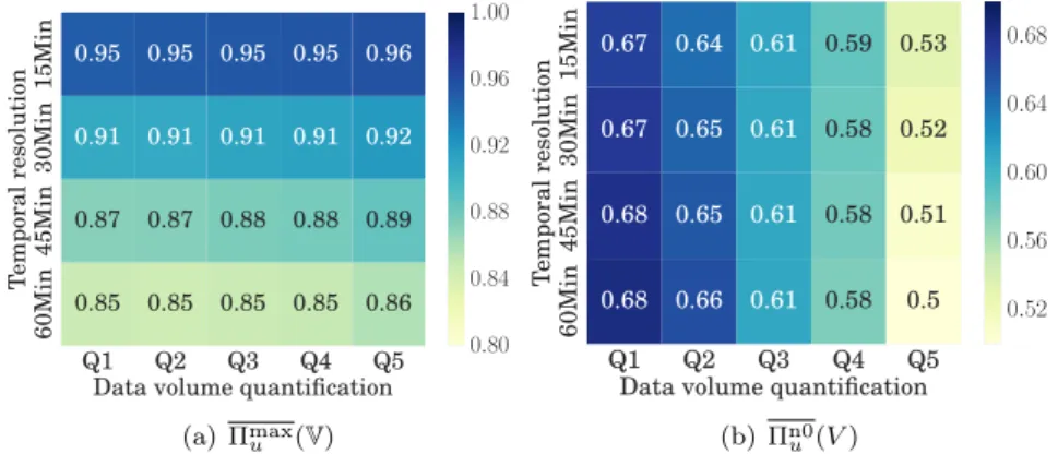
60Min 45Min 30Min 15Min Temporal resolution 0.85 0.85 0.85 0.85 0.86 0.87 0.87 0.88 0.88 0.89 0.91 0.91 0.91 0.91 0.92 0.95 0.95 0.95 0.95 0.96 0.80 0.84 0.88 0.92 0.96 1.00 (a) Πmax u (V) Q1 Q2 Q3 Q4 Q5 Data volume quantification
60Min 45Min 30Min 15Min Temporal resolution 0.68 0.66 0.61 0.58 0.5 0.68 0.65 0.61 0.58 0.51 0.67 0.65 0.61 0.58 0.52 0.67 0.64 0.61 0.59 0.53 0.52 0.56 0.60 0.64 0.68 (b) Πn0 u (V )
Figure 4: (a) Heatmap of the median predictability upper bound Πmax
u (V) for different
quantiza-tions of time and traffic volume. (b) Heatmap of the median predictability upper bound Πn0
u (V )
for different quantizations of time and traffic volume.
Let us start by considering the PDF of Hrand
u (V )in Fig. 3(b). Its range indicates that an
equiprobable distribution of traffic volume during each time interval can be represented with three bits. This phenomenon is normal, as we consider eight traffic volume quantization levels
as our default setting. When the temporal-uncorrelated entropy, i.e., Hunc
u (V ), is concerned, a
sizable shift of probability occurs. The uncertainty decreases to 2Hunc
u (V ) = 21.63 ≈ 3. Under
this model, each user tends to generate traffic that is described by just three quantization levels out of the eight available. For instance, at each time interval, a user may generate traffic by one order of MB or tens of MB, or stay idle; but typically she will not generate smaller or larger traffic volumes. The same holds for users who generate, e.g., order-of-KB or order-of-GB traffic. Ultimately, a reduced entropy rate implies higher regularity in the mobile traffic demand.
Interestingly, idle time intervals do not bias such regularity. Indeed, the PDF of Hn0
u (V )
overlaps well to that of Hunc
u (V ), suggesting that the considerations above also hold when only
time intervals with data sessions are considered. However, our main result is the significant
shift presented by the PDF of Hu(V), which is amassed around a value 0.97. When taking
the temporal ordering of data sessions into account, one can reduce the uncertainty to just two quantization levels.
The probability distributions in Fig. 3(c) confirm these findings and provide upper numerical bounds to the predictability of the mobile data traffic demand generated by individual
sub-scribers. We observe that Πrand
u (V ) peaks at 0.16, i.e., it is very hard to guess the volume of
traffic generated by such a stochastic model. The predictability grows for Πunc
u (V )and Πn0u (V ),
which peak at 0.69 and 0.66, respectively. More importantly, Πmax
u (V) indicates that the demand
of a subscriber can be possibly predicted within 85% accuracy on average. It means that in only
15% of the time does the subscriber generate a traffic volume in a manner that appears to be
random, but in the remaining 85% of the time, we could hope to predict her volume. This re-sult proves, for the first time, that the traffic volume which subscribers generate via their mobile devices is highly predictable.
The results in Fig. 3(b) and Fig. 3(c) refer to the case where the individual mobile data traffic is represented with a temporal resolution of 60 minutes and volume quantization Q2. In fact, data granularity has been shown to have a significant impact in the predictability of mobility [30]. We thus explore if the same is true in the case of predictability of the mobile data traffic demand. The heatmaps in Fig. 4(a) and in Fig. 4(b) show the median of the upper bound on the mobile demand predictability, over four temporal and five traffic volume quantization levels. The two
plots refer to Πmax
u (V) and Πn0u (V ), respectively.
In Fig. 4(a), we observe that Πmax
u (V) is not significantly affected by the traffic volume
quan-tization, i.e., our results appear to have general validity under different levels of accuracy in the representation of the mobile demand. In contrast, surprisingly, it grows with finer-grained temporal resolutions. The reason is that more idle intervals appear as the temporal resolution is increased; these idle intervals tend to dominate the real-world distribution of mobile data traf-fic, reducing the entropy and improving the overall predictability but hiding the predictability
12 Guangshuo Chen, Sahar Hoteit, Aline Carneiro Viana, Marco Fiore, Carlos Sarraute
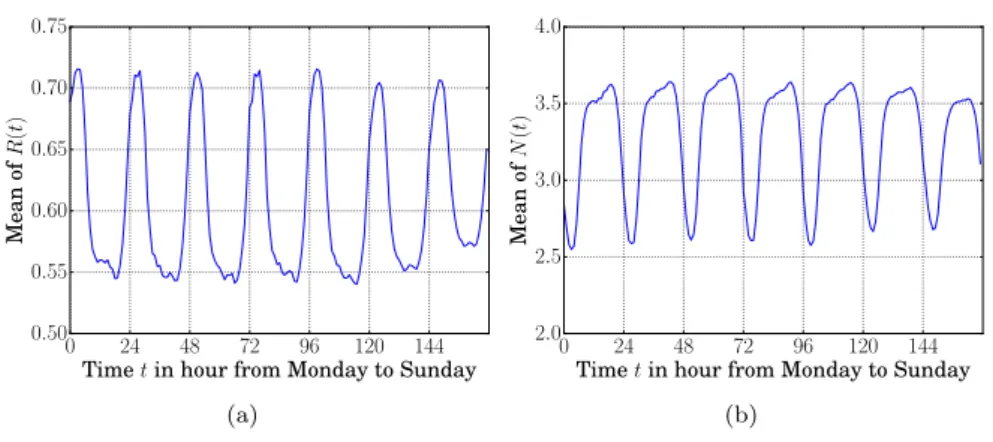
0 24 48 72 96 120 144 Time t in hour from Monday to Sunday 0.50 0.55 0.60 0.65 0.70 0.75 Mean of R (t ) (a) 0 24 48 72 96 120 144 Time t in hour from Monday to Sunday 2.0 2.5 3.0 3.5 4.0 Mean of N (t ) (b)
Figure 5: Temporal dynamics of individual mobile data traffic volume, during the average week. (a) Regularly R(t). (b) Number of observed levels N(t).
of non-idle intervals. This is confirmed by Fig. 4(b): Πn0
u (V ), which only accounts for non-idle
time intervals, is slightly affected by variations in the time granularity. Instead, it is strongly dependent on the traffic volume quantization, an artifact of the lack of temporal correlation in
this model, which disappears in Πmax
u (V).
5.3
Temporal variability
It is well-known that the demand generated by mobile phone subscribers is time-dependent [17]. Thus, a relevant question is whether the predictability of mobile data traffic similarly undergoes temporal variations. Nevertheless, entropy does not allow a detailed view of such temporal variation.
To that end, we compute, for each user and on an hourly basis, the regularity R(t), i.e., the probability that the user generates the most likely traffic volume observed during each hour. Similarly, we define N(t) as the number of unique traffic volume levels observed at each hour. Regularity provides a lower bound on the predictability, as it ignores the temporal correlation of subscribers’ traffic demand patterns [4, 24], and is typically inversely correlated with N(t). R(t) and N(t) can be seen as proxies of the predictability and entropy rate.
Fig. 5 shows the evolution of R(t) and N(t) over the average week. We remark a clear circadian rhythm. At night, the mean of R(t) rises to approximately 0.7, meaning that, on average, the subscriber’s demand matches the most likely traffic volume around 70% of the time. During the morning, working hours, and evening, R(t) drops to 0.55. N(t) shows opposite trends, as expected. As R(t), N(t) (as tied to the predictability) varies significantly over time as well. However, we do not observe significant variations from one day to another, which suggests that mobile data traffic volume predictability is not only imposed by the working schedule but is intrinsic to more generic human activities.
5.4
Variability across subscriber types
Our datasets let us explore several additional dimensions of the traffic volume predictability. These dimensions are related to the nature of the subscriber. The results are shown in Fig. 6 and discussed below.
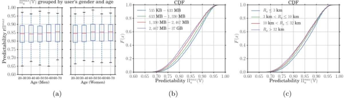
• Age and gender. The age and gender of the mobile user are known to affect the way mobile services are consumed. However, Fig. 6(a) shows that these do not affect in a remarkable manner the predictability of the traffic volume. Hence, age- and gender-induced behaviors remain similarly predictable when it comes to the traffic volume.
• Overall mobile data traffic volume consumption. We categorize users into four groups, according to their data consumption during the 92 days of the data collection period. Each group consists of 25% of the observed users. As shown in Fig. 6(b), the predictability
Πmax
u (V) tend to decrease as the data volume increases. Yet, the mean of Πmaxu (V) is 85.5%
20-30 30-40 40-50 50-60 60-70 Age (Men) 0.60 0.65 0.70 0.75 0.80 0.85 0.90 0.95 1.00 Predictability rΠ max 20-30 30-40 40-50 50-60 60-70 Age (Women) Πmax
u (V) grouped by user’s gender and age
(a) 0.60 0.65 0.70 0.75 0.80 0.85 0.90 0.95 1.00 Predictability Πmax u (V) 0.0 0.2 0.4 0.6 0.8 1.0 F (x ) CDF 535KB − 633 MB 633MB − 1, 330 MB 1, 330MB − 2, 467 MB 2, 467MB − 37 GB (b) 0.60 0.65 0.70 0.75 0.80 0.85 0.90 0.95 1.00 Predictability Πmax u (V) 0.0 0.2 0.4 0.6 0.8 1.0 F (x ) CDF Rg≤ 3 km 3km < Rg≤ 10 km 10km < Rg≤ 32 km Rg> 32km (c)
Figure 6: (a) Boxplot of Πmax
u (V) categorized by user’s age and gender. Each box denotes the
median, 25th
− 75thpercentiles, and minimum and maximum values. (b) CDF of Πmax
u (V), when
users are separated according to the overall mobile data traffic volume recorded they generate during the measurement period of 92 days. Four groups are considered: 535 KB − 633 MB,
633MB − 1, 330 MB, 1, 330 MB − 2, 467 MB, and 2, 467 MB − 37 GB. Each group contains 25%
of the observed users. (c) CDF of Πmax
u (V), when users are separated according to their level of
mobility. Four ranges of radius of gyration are considered, mapping to sedentary (Rg ≤ 3km),
urban (3 km < Rg ≤ 10 km), peri-urban (10 km < Rg ≤ 32 km), and long-range commuting
(Rg> 32km) profiles.
in the group of 535 KB − 674 MB and 83.1% in the group of 2, 553 MB − 37 GB. The difference is thus small and can be imputed to the fact that a larger amount of data naturally entails more complex dynamics as well as may be characterized by a lower regularity. We conclude that the overall amount of generated traffic only marginally impacts the potential predictability of traffic volumes.
• Mobility level. Some correlations between mobility and mobile service usage were observed in the literature [20, 15, 18]. We study whether this occurs with mobile data traffic volume predictability as well. To that end, we compute, for each user, the radius of gyration [31],
i.e., the root mean square distance of all recorded locations with respect to their center
of mass. The radius of gyration provides a measure of the overall level of mobility of an individual and allows classifying subscribers into the following categories: sedentary,
urban, peri-urban, and long-range commuters [32]. Fig. 6(c) presents the CDF of Πmax
u (V)
computed on each user category. Again, there exists a slight shift towards lower values in
the Πmax
u (V) distribution, as the level of mobility grows. However, the variation is minimal,
at 1.3% between commuters and sedentary users. This implies that less mobile users may have slightly more regular data traffic patterns, yet the difference is marginal.
In conclusion, we find no significant correlations between dominant subscribers’ features and the predictability of the mobile data traffic volume they generate. In fact, all plots in Fig. 6
indicate that the heterogeneity of Πmax
u (V) across all users is fairly low: the high predictability
of traffic volume is a property shared throughout the whole user population.
6
Joint predictability of traffic and mobility
In this section, we push our analysis further, and study the joint predictability of future mobile data traffic volume and visited locations, on a per-user basis. In other words, we investigate how predictable is the combination of how much traffic is generated by a mobile phone subscriber and where this happens. Note that the temporal dimension, i.e., when the mobile data traffic is consumed, is implicitly taken into account by the temporal correlation in the definition of the predictability upper bound. Overall, our analysis provides a first comprehensive understanding of whether it is possible to anticipate when, where, and how much mobile data traffic is generated by individual subscribers.
14 Guangshuo Chen, Sahar Hoteit, Aline Carneiro Viana, Marco Fiore, Carlos Sarraute 0 1 2 3 4 5 6 7 8 Entropy H 0.0 0.2 0.4 0.6 0.8 1.0 1.2 1.4 P (H ) PDF Hrand u (L) Hunc u (L) Hu(L) (a) Entropy 0.0 0.2 0.4 0.6 0.8 1.0 Upper limit of predictablity Π 0 5 10 15 20 25 P (Π) PDF Πrand u (L) Πunc u (L) Πmax u (L) (b) Predictability
Figure 7: (a) The distribution of the random entropy Hrand
u (L), the temporal-uncorrelated
en-tropy Hunc
u (L)and the entropy rate Hu(V) across the observed 45, 832 users. (b) The distribution
of the upper bounds on the predictability Πrand
u (L), Πuncu (L)and Πmaxu (L) across the observed
users.
6.1
Methodology
We build on knowledge of each user’s sequences of traffic volumes Svol
u and locations S
loc
u , and
compute several measures of interest, as follows.
Predictability of mobility. We consider a stationary stochastic process L = {Li,· · · , LT}
which represents a sequence of locations Li, recorded for a given user at each time interval i.
In a similar way to what done in Sec. 5.1 for the mobile data traffic volume, we leverage Sloc
u to
calculate three entropy rate variants on subscribers’ mobility: the random entropy Hrand
u (L), the
temporal-uncorrelated entropy Huunc(L), and the actual entropy rate Hu(L). These allow
com-puting their corresponding upper bounds on the predictability Πrand
u (L), Πuncu (L), and Πmaxu (L).
These are the same exact measures used in [4], and are used to study to what extent user mobility can be anticipated when considered in isolation.
Predictability of joint mobility and traffic volume. The traffic process V and
mobil-ity process L are combined into a single joint process M = {(V1, L1),· · · , (VT, LT)}.
Cor-respondingly, from a measurement data perspective, Svol
u and Slocu are merged into Smixu =
{(v1
u, l1u),· · · , (vTu, lTu)}, for each user u. The following variants of the entropy rate are calculated
on Smix
u ∀u ∈ U. The temporal-uncorrelated entropy Huunc(V, L)≡ −
P
v∈V,l∈Lp(v, l) log2p(v, l)
determines the heterogeneity deriving from simply considering the user’s location and traffic
vol-ume together. The joint actual entropy rate Hu(V, L) is defined as the actual entropy rate of
the joint stationary process M. It expresses the combined uncertainty of a user’s location and traffic volume at a given time instant, considering his previous history of movements and mobile
service usage. The corresponding predictability upper bounds Πunc
u (V, L) and Π
max
u (V, L) are
calculated as detailed in Sec. 3.
Predictability of data traffic conditioned on mobility: This is a simplified variant of the
joint case above, where the two dimensions of traffic volume and mobility are not considered at once, but the former is conditioned on the latter. In other words, only the traffic volume is forecast, assuming knowledge of the past and current locations. Formally, the conditional
entropy rate is Hu(V|L) ≡ Hu(V, L) − Hu(L), and the temporal-uncorrelated conditional entropy
is Hunc
u (V|L) ≡ Huunc(V, L)−Huunc(L). The predictability upper bounds mapping to each entropy
rate are Sloc
u and Svolu , respectively.
6.2
User mobility in isolation
We first investigate how predictable is individual mobility when considered in isolation. This means to re-run the exact same study presented in [4] on our CDR dataset. The results, in Fig. 7, are consistent with those in the literature, yet they present interesting slight variations that are discussed next.
Fig. 7(a) presents the PDF of the entropy rates Hrand
u (L), Huunc(L)and Hu(L). P (Hurand(L))
and P (Hunc
u (L)) are bell-shaped and have statistical measures that are close to those found
in [4]. Specifically, Hrand
u (L)has a mean of approximately 5 bit, indicating that a user’s entire
movement space is composed of 2Hurand(L)
≈ 32 cells on average. Also, Hrand
u (L)has a significant
variance, i.e., the geographical span of movements varies widely from person to person in our
dataset. The mean is higher in the case of Hunc
u (L), at ≈ 2.4 bit. Users tend to favor some
locations over others, and keeping this into consideration allows making more accurate forecasts
on the next location they will visit: the uncertainty shrinks to just 2Huunc(L)
≈ 5 locations on average.
However, the most interesting result is the distribution of Hu, which, unlike what found in
previous studies, is the composition of two bell-shaped distributions with peaks at around 0.03 and 0.65, respectively. The second peak implies that the uncertainty in anticipating the next
cell of a subscriber is limited to 2Hu(L) ≈ 2 options; this is consistent with what reported in [4].
The first peak is symptomatic of an even lower indecision: in fact, 20.03
≈ 1, i.e., there are situations where the next location of a user is almost certain. We ascribe this result to the fact that we complete the original CDR data using the stop-by-spothome approach, as discussed in Sec. 4.2. On the one hand, the data completion places individuals at one single cell (i.e., their home location) for long, continuative periods of time: there is thus little uncertainty about where subscribers are at night. On the other hand, raw CDR data was employed in [4], which could not capture the low entropy rate associated with the lack of movement overnight.
Fig. 7(b) shows the PDF of the predictability upper bounds Πrand
u (L) and Πuncu (L),
corre-sponding to the entropy rates above. The results are consistent: Πrand
u (L) has a distribution
that is narrowly peaked at very low values, while Πunc
u (L)yields better predictability but widely
varies significantly among individuals. While Πrand
u (L)distribution is in agreement with those
originally presented in [4], our results on the Πunc
u (L)distribution are instead much better (i.e.,
Πunc
u (L) = 0.6, instead of 0.3 as reported in [4, Fig. 2.B]), what is due to our CDR dataset
completion process. More significant differences emerge instead for Πmax
u (L), with two distinct
peaks at Πmax
u = 0.94and Π
max
u = 0.99. The former value is very close to the Π
max
u = 0.93
re-ported in [4]. The second peak is again due to the CDR dataset completion process, as explained above. We verified this hypothesis by running experiments on our CDR dataset without data
completion: in this case, we obtain a bell-shaped distribution of Πmax
u (L) peaked at 0.93, and
the second peak disappears. In all cases, our results confirm that user mobility alone is highly predictable.
6.3
Mobile data traffic volume and mobility
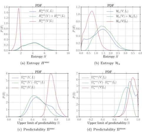
We now consider the uncertainty and predictability of traffic volume and mobility at once. Our results are summarized in Fig. 8, which portrays PDFs for different ways of bringing together the two dimensions of traffic volumes and locations. Specifically, each plot contains three curves: (i) the joint entropy or associated predictability, (ii) the sum of entropy rates measured for traffic volume and mobility separately, and (iii) the conditional entropy rate or associated predictability. The second curve represents the uncertainty (or predictability) in the case the stochastic processes driving mobility and traffic volume consumption are independent of each other. Fig. 8(a) and Fig. 8(c) refer to temporal-uncorrelated versions, whereas Fig. 8(b) and Fig. 8(d) concern our actual measures of interest.
A first interesting remark is that Hunc
u (V, L) and Huunc(V ) + Huunc(L)in Fig. 8(a), and
con-sequently Πunc
u (V, L)and Πuncu (V )· Πuncu (L) in Fig. 8(c), are nearly indistinguishable. Instead,
Hu(V, L) and Hu(V)+Hu(L) in Fig. 8(b), and consequently Πumax(V, L) and Πmaxu (L)·Πmaxu (V) in
Fig. 8(d), show significant differences. Hence, there exists some correlation between the mobility and traffic volume consumption processes, and such correlation mainly emerges when consider-ing – and it is thus driven by – the temporal orderconsider-ing of events. As observed in Fig. 8(d), a joint prediction of the next consumed amount of traffic and of the future location where this occurs can yield a better accuracy than forecasting the two separately, when knowledge of the
previous actions of the individual is taken into account. The shift between Πmax
u (L) · Πmaxu (V)
and Πmax
u (V, L) is of 10% on average.
More importantly, we note that the mean value of Πmax
u (V, L) is at 0.88, with the probability
mass above 0.8 and a noticeable peak at 0.98. Therefore, our main conclusion is that it is possible to anticipate how much mobile data traffic (as an order of magnitude) will be consumed by a
16 Guangshuo Chen, Sahar Hoteit, Aline Carneiro Viana, Marco Fiore, Carlos Sarraute 0 2 4 6 8 10 Entropy H 0.0 0.2 0.4 0.6 0.8 1.0 1.2 1.4 1.6 P (H ) PDF Hunc u (V, L) Hunc u (V ) + Huunc(L) Hunc u (V|L)
(a) Entropy Hunc
0.0 0.5 1.0 1.5 2.0 2.5 3.0 3.5 4.0 Entropy H 0.0 0.2 0.4 0.6 0.8 1.0 1.2 P (H ) PDF Hu(V, L) Hu(V) + Hu(L) Hu(V|L) (b) Entropy Hu 0.0 0.2 0.4 0.6 0.8 1.0 Upper limit of predictablity Π 0 1 2 3 4 5 6 P (Π) PDF Πunc u (V, L) Πunc u (V )· Πuncu (L) Πunc u (V|L) (c) Predictability Πunc 0.0 0.2 0.4 0.6 0.8 1.0 Upper limit of predictablity Π 0 1 2 3 4 5 6 7 P (Π) PDF Πmax u (V, L) Πmax u (V) · Πmaxu (L) Πmax u (V|L) (d) Predictability Πmax
Figure 8: (a) Distributions of the different flavors of temporal-uncorrelated entropies: Hunc
u (V, L),
Huunc(V ) + Huunc(L) and Huunc(V|L). (b) Distributions of the different flavors of entropy rates:
Hu(V), Hu(V) + Hu(V) and Hu(V|L). (c) Distributions of the predictability upper bounds
Πuncu (V, L), Πuncu (L)· Πuncu (L)and Πuncu (V|L) based on the corresponding temporal-uncorrelated
entropies. (d) Distributions of the predictability upper bounds Πmax
u (V, L), Πmaxu (V) · Πmaxu (L)
and Πmax
u (V|L) based on the corresponding entropy rates.
given subscriber and where this will occur in a very effective manner (i.e., with an 88% accuracy on average), by knowing the past history of activities of the target individual.
If the available information about each user increases, and the location information can be precisely established (e.g., because mobility occurs at much longer timescales than service consumption, or we know that the user has especially deterministic movement pattern), one can remove the uncertainty about the mobility dimension. In fact, the knowledge about the past and current locations can be then leveraged to even improve the accuracy of the prediction, which occurs in both temporal-uncorrelated and actual cases, as shown in Fig. 8. The plot
in Fig. 8(d) also portrays the range of the predictability gain: by comparing Πmax
u (V|L) with
Πmax
u (V) in Fig. 3(c), we observe that including location information in the prediction process
allows forecasting the future consumption of mobile data traffic with 5% higher accuracy, pushing the overall performance from 85% to 90%. Hence, our second conclusion is that using knowledge of the spatio-temporal trajectories of subscribers can further improve the design of a prediction model targeting individual traffic volume consumption. Yet, the gain is not dramatic with respect to a technique that only relies on temporal information.
7
Discussion
Understanding the cause of the high (joint) predictability observed in Sec. 6 is relevant to the design of practical solutions for the prediction of mobile subscriber behavior.
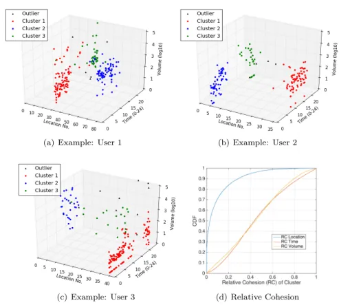
To investigate this issue, we map each user’s Internet sessions into a three-dimensional space of location, time, and volume. Each session becomes then a point p(l, t, v) into this space. To
represent the location obtained from Sloc
u using one dimension, for each user, we use the Optics
(a) Example: User 1 (b) Example: User 2
(c) Example: User 3 (d) Relative Cohesion
Figure 9: (a)(b)(c) Examples of mapping a user’s sessions mapped the three-dimensional space. (b) CDF of each cluster’s relative cohesion on the three dimensions. Figure best viewed in colors.
algorithm [33] to cluster spatially close locations appearing in the Sloc
u , and then use the node
identifier as a location value l instead of the coordinate (lat, lon). Time t is expressed by hours with decimals from 0 to 24, where the date is ignored. Finally, volume v is the magnitude of the traffic volume, i.e., log10(·).
In this three-dimensional space, we can clearly observe how a user generates mobile Internet sessions. Examples are shown in Fig. 9. For the user 1 in Fig. 9(a), sessions are aggregated mainly on two major locations (i.e.with IDs 30 and 60), probably mapping to home and working place according to their time of visit. Besides, sessions containing large data traffic (> 10MB) mostly occur at the location 30 during nighttime. In Fig. 9(b) and 9(c), though the data traffic consumption of the two users are different, we also observe similar aggregating patterns of their sessions.
Overall, we find that the 3D space representation of user’s sessions is typical for the vast majority of users. Hence, we investigate quantitatively the clustering of such points. For that, we use DBScan [34] to cluster each user’s sessions in the three-dimensional space. The algorithm parameters minP ts and Eps are set to minP ts = 4 and Eps = 0.25 after extensive tests. For the
clustering, a weighted euclidean distance is measured between every two points p1(l1, t1, v1)and
p2(l2, t2, v2), where the distance of each dimension is computed as follows: (i) for the location,
dist(location)(p
1, p2) = ωl|l1−l2|geoin kilometers; (ii) for the time, dist(time)(p1, p2) = ωt|t1−t2|
in hours; (iii) for the volume, dist(volume)(p
1, p2) = ωv|v1− v2| (|log10VolVol1
2|). Each distance
is normalized by the largest 1% of the distances on that dimension through the parameters ωl,
ωt and ωv, respectively. Examples of the result returned by DBScan are shown in Fig. 9, where
colors are used to denote different clusters of session points.
For each cluster, we use the relative cohesion (RC) to quantify the contribution of each
dimension to a given cluster as RC(∗) = Pp∈Cdist
(∗)(p,c)2
P
p∈Cdist(p,c)2 , where C and c represents the cluster
and its centroid c = (lcentroid, tmean, vmean). The RCs of the three dimensions satisfy RC(loc)+
18 Guangshuo Chen, Sahar Hoteit, Aline Carneiro Viana, Marco Fiore, Carlos Sarraute significantly smaller than the other two dimensions, we can say this dimension is contributing the most to the creation of the cluster.
Fig. 9(d) shows the distributions of RC along the three dimensions. The most striking be-havior is the much lower RC in space than time or traffic volume: i.e.where a user is drives the creation of the majority of clusters. In other words, the location of a mobile user has a high probability to trigger some routine service consumption activity; hence, anticipating the future location of a subscriber should be the first target of a solution aiming at predicting mobile user activity. However, we also observe that locations alone do not explain all clusters. A non-negligible fraction of clusters showing high RC in space and low RC in time and traffic volume are also present in several cases. We conclude that the three dimensions are complementary, and, although with different weights, are all important for an accurate prediction of the behavior of mobile subscribers. This is consistent with – and explains – our results on the high joint predictability of temporally correlated visited locations and consumed traffic.
8
Conclusions
To the best of our knowledge, this is the first work to (i) show the maximum predictability of personal mobile data traffic volume and (ii) jointly consider user’s location and mobile service usage in a per-user predictability analysis. We found an upper limit on such predictability, demonstrating that it is possible to anticipate upper bounds on how much traffic a subscriber will generate, as well as where he will do so, with 88% accuracy on average, by leveraging historical information about the user. This result is possible thanks to correlations between visited locations and traffic volumes: indeed, trying to analyze predictability of traffic volumes in isolation reduces the accuracy to 85%. If the location information is instead known and used at the analysis, the mean precision grows to 90%. Our results indicate that there is a large space for predicting mobile data traffic and adapting network optimizing solutions based on the latter, such as caching and prefetching.
To further analyze the predictability and its limits, it requires a more fine-grained view of users behavior (e.g., types of content or device, contextual information), which we will consider in future works. In addition, we plan to make explicit predictions on users’ mobile data traffic consumption, turning the predictability identified in our study into actual traffic predictions.
References
[1] Diala Naboulsi, Marco Fiore, Stephane Ribot, and Razvan Stanica. Large-scale Mobile Traffic Analysis: a Survey. IEEE Communica-tions Surveys & Tutorials, PP(99):1–1, 2015.
[2] William Su, S-J Lee, and Mario Gerla. Mobility prediction in wireless networks. In IEEE MILCOM 2000, volume 1, pages 491–495. IEEE, 2000.
[3] Pubudu N Pathirana, Andrey V Savkin, and Sanjay Jha. Mobility modelling and trajectory prediction for cellular networks with mobile base stations. In ACM MobiHoc 2003c, pages 213–221. ACM, 2003.
[4] C Song, Z Qu, N Blumm, and Albert-László Barabási. Limits of Predictability in Human Mobility. Science, 327(5968):1018–1021, February 2010.
[5] David G. Taylor and Michael Levin. Predicting mobile app usage for purchasing and information-sharing. International Journal of Retail & Distribution Management, 42(8):759–774, 2014.
[6] Wee-Seng Soh and Hyong S Kim. Qos provisioning in cellular networks based on mobility prediction techniques. IEEE Communications Magazine, 41(1):86–92, 2003.
[7] Henrik Petander. Energy-aware network selection using traffic estimation. In ACM MICNET 2009, pages 55–60. ACM, 2009.
[8] Vasilios A Siris and Dimitrios Kalyvas. Enhancing mobile data offloading with mobility prediction and prefetching. ACM SIGMOBILE Mobile Computing and Communications Review, 17(1):22–29, 2013.
[9] Zhiyuan Li, Junlei Bi, and Siguang Chen. Traffic prediction-based fast rerouting algorithm for wireless multimedia sensor networks. International Journal of Distributed Sensor Networks, 2013.
[10] Xuan Zhou, Zhifeng Zhao, Rongpeng Li, Yifan Zhou, and Honggang Zhang. The predictability of cellular networks traffic. In IEEE ISCIT 2012, pages 973–978. IEEE, 2012.
[11] Rongpeng Li, Zhifeng Zhao, Xuan Zhou, Jacques Palicot, and Honggang Zhang. The prediction analysis of cellular radio access network traffic: From entropy theory to networking practice. IEEE Communications Magazine, 52(6):234–240, 2014.
[12] Sven AM Ostring and Harsha Sirisena. The influence of long-range dependence on traffic prediction. In IEEE ICC 2001, volume 4, pages 1000–1005. IEEE, 2001.
[13] M. E. Crovella and A. Bestavros. Self-similarity in world wide web traffic: evidence and possible causes. IEEE/ACM Transactions on Networking, 5(6):835–846, Dec 1997.
[14] Aimin Sang and San-qi Li. A predictability analysis of network traffic. Computer networks, 39(4):329–345, 2002.
[15] Utpal Paul, Anand Prabhu Subramanian, Milind M Buddhikot, and Samir R Das. Understanding traffic dynamics in cellular data networks. INFOCOM, pages 882–890, 2011.
[16] M Zubair Shafiq, Lusheng Ji, Alex X Liu, and Jia Wang. Characterizing and modeling internet traffic dynamics of cellular devices. ACM SIGMETRICS Performance Evaluation Review, 39(1), June 2011.
[17] Eduardo Mucelli Rezende Oliveira, Aline Carneiro Viana, Kolar Purushothama Naveen, and Carlos Sarraute. Mobile data traffic modeling: Revealing temporal facets. Computer Networks, 112:176–193, 2017.
[18] H H Jo, M Karsai, J Karikoski, and K Kaski. Spatiotemporal correlations of handset-based service usages. EPJ Data Science, 1:1–18, 2012.
[19] Khushboo Shah, Stephan Bohacek, and Edmond A Jonckheere. On the predictability of data network traffic. In Proceedings of the American Control Conference, volume 2, pages 1619–1624, 2003.
[20] Ionut Trestian, Supranamaya Ranjan, Aleksandar Kuzmanovic, and Antonio Nucci. Measuring serendipity: Connecting people, locations and interests in a mobile 3g network. In ACM SIGCOMM 2009, IMC ’09, pages 267–279, New York, NY, USA, 2009. ACM.
[21] Thomas M Cover and Joy A Thomas. Elements of information theory. John Wiley & Sons, 2012.
[22] Thomas Schürmann and Peter Grassberger. Entropy estimation of symbol sequences. Chaos: An Interdisciplinary Journal of Nonlinear Science, 6(3):414–427, September 1996.
[23] Hui Zang and Jean C Bolot. Mining call and mobility data to improve paging efficiency in cellular networks. In ACM MobiCom 2007, pages 123–134, New York, USA, September 2007. ACM.
[24] C Song, Z Qu, N Blumm, and Albert-László Barabási. Limits of Predictability in Human Mobility Supplementary Material. Science Online.
[25] Xin Lu, Erik Wetter, Nita Bharti, Andrew J Tatem, and Linus Bengtsson. Approaching the Limit of Predictability in Human Mobility. Scientific reports, 3:2923, October 2013.
[26] Jingyuan Wang, Yu Mao, Jing Li, Zhang Xiong, and Wen-Xu Wang. Predictability of Road Traffic and Congestion in Urban Areas. PloS one, 10(4):e0121825, 2015.
[27] Salvatore Scellato, Mirco Musolesi, Cecilia Mascolo, Vito Latora, and Andrew T Campbell. NextPlace: A Spatio-temporal Prediction Framework for Pervasive Systems. Pervasive, 6696(Chapter 10):152–169, 2011.
[28] Ioannis Kontoyiannis, Paul H Algoet, Yu M Suhov, and Abraham J Wyner. Nonparametric entropy estimation for stationary processes and random fields, with applications to english text. IEEE Transactions on Information Theory, 44(3):1319–1327, 1998.
[29] Sahar Hoteit, Guangshuo Chen, Aline Viana, and Marco Fiore. Filling the gaps: On the completion of sparse call detail records for mobility analysis. In ACM Chants, 2016.
[30] G. Smith, R. Wieser, J. Goulding, and D. Barrack. A refined limit on the predictability of human mobility. In IEEE PerCom 2014, pages 88–94, March 2014.
[31] Marta C González, César A Hidalgo, and Albert-László Barabási. Understanding individual human mobility patterns. Nature, 453(7196):779–782, June 2008.
[32] Sahar Hoteit, Stefano Secci, Stanislav Sobolevsky, Carlo Ratti, and Guy Pujolle. Estimating human trajectories and hotspots through mobile phone data. Computer Networks, 64:296–307, 2014.
[33] Mihael Ankerst, Markus M Breunig, Hans-Peter Kriegel, and Jörg Sander. Optics: ordering points to identify the clustering structure. In ACM Sigmod Record, volume 28, pages 49–60. ACM, 1999.
RESEARCH CENTRE SACLAY – ÎLE-DE-FRANCE 1 rue Honoré d’Estienne d’Orves Bâtiment Alan Turing
Campus de l’École Polytechnique 91120 Palaiseau
Publisher Inria
Domaine de Voluceau - Rocquencourt BP 105 - 78153 Le Chesnay Cedex inria.fr