Publisher’s version / Version de l'éditeur:
Vous avez des questions? Nous pouvons vous aider. Pour communiquer directement avec un auteur, consultez la première page de la revue dans laquelle son article a été publié afin de trouver ses coordonnées. Si vous n’arrivez pas à les repérer, communiquez avec nous à [email protected].
Questions? Contact the NRC Publications Archive team at
[email protected]. If you wish to email the authors directly, please see the first page of the publication for their contact information.
https://publications-cnrc.canada.ca/fra/droits
L’accès à ce site Web et l’utilisation de son contenu sont assujettis aux conditions présentées dans le site LISEZ CES CONDITIONS ATTENTIVEMENT AVANT D’UTILISER CE SITE WEB.
Laboratory Memorandum; no. LM-2004-14, 2004
READ THESE TERMS AND CONDITIONS CAREFULLY BEFORE USING THIS WEBSITE.
https://nrc-publications.canada.ca/eng/copyright
NRC Publications Archive Record / Notice des Archives des publications du CNRC :
https://nrc-publications.canada.ca/eng/view/object/?id=9eb7368f-89ad-4061-b30a-3ebb649864df https://publications-cnrc.canada.ca/fra/voir/objet/?id=9eb7368f-89ad-4061-b30a-3ebb649864df
NRC Publications Archive
Archives des publications du CNRC
For the publisher’s version, please access the DOI link below./ Pour consulter la version de l’éditeur, utilisez le lien DOI ci-dessous.
https://doi.org/10.4224/8895739
Access and use of this website and the material on it are subject to the Terms and Conditions set forth at
Validation of GEDAP Programs "Wavetran" and "Boat-Wave"
Institute for Ocean Technology
Institut des
technologies oc ´eaniques
Laboratory Memorandum
LM-2004-14
Validation of Gedap Programs 'Wavetran' and 'Boat-Wave'
D. Cumming and L. Mak
June 2004
DOCUMENTATION PAGE
REPORT NUMBER
LM-2004-14
NRC REPORT NUMBER DATE
June 2004
REPORT SECURITY CLASSIFICATION
Unclassified
DISTRIBUTION
Unlimited
TITLE
VALIDATION OF GEDAP PROGRAMS ‘WAVETRAN’ AND ‘BOAT_WAVE’
AUTHOR(S)
D. Cumming and L. Mak
CORPORATE AUTHOR(S)/PERFORMING AGENCY(S)
Institute for Ocean Technology, National Research Council, St. John’s, NL
PUBLICATION
N/A
SPONSORING AGENCY(S)
Institute for Ocean Technology, National Research Council, St. John’s, NL
IMD PROJECT NUMBER
42_960_26
NRC FILE NUMBER KEY WORDS
Software, WAVETRAN, BOAT_WAVE
PAGES iv, 12, App. A-D FIGS. 16 TABLES 9 SUMMARY
This report documents the validation, using realistic physical wave data acquired in the Institute for Ocean Technology (IOT) Offshore Engineering Basin (OEB), of GEDAP programs ‘WAVETRAN’ and ‘BOAT_WAVE’. ‘WAVETRAN’ is used to translate unidirectional regular or irregular wave data from a stationary wave probe to another stationary point using linear theory. ‘BOAT_WAVE’ is used to translate unidirectional regular or irregular wave data from a stationary wave probe to a defined point on a moving model using linear theory. An attempt will be made to define an envelope for valid use of the software.
ADDRESS National Research Council
Institute for Ocean Technology Arctic Avenue, P. O. Box 12093 St. John's, NL A1B 3T5
Institute for Ocean Institut des technologies
Technology océaniques
VALIDATION OF GEDAP PROGRAMS ‘WAVETRAN’ AND
‘BOAT_WAVE’
LM-2004-14
D. Cumming, L. Mak
LM-2004-14
TABLE OF CONTENTS
List of Tables ... iv
List of Figures ... iv
List of Symbols and Abbreviations ... v
1.0 INTRODUCTION...1
2.0 BACKGROUND ...1
3.0 DESCRIPTION OF THE OFFSHORE ENGINEERING BASIN ...1
4.0 DESCRIPTION OF GEDAP PROGRAMS ‘WAVETRAN’ AND ‘BOAT_WAVE’ ...2
5.0 OEB TEST CONFIGURATIONS ...3
6.0 ‘WAVETRAN’ VALIDATION ...5
7.0 ‘BOAT_WAVE’ VALIDATION ...7
8.0 DISCUSSION...9
8.1 ‘WAVETRAN’ Validation Results...9
8.2 ‘BOAT_WAVE’ Validation Results...10
9.0 CONCLUSIONS AND RECOMMENDATIONS ...11
9.1 Programs ‘WAVETRAN’ and ‘BOAT_WAVE’ ...11
9.2 Other Recommendations ...11
10.0 ACKNOWLEDGEMENTS ...12
11.0 REFERENCES...12
APPENDIX A: Description of the Offshore Engineering Basin APPENDIX B: Description of the QUALISYS System
APPENDIX C: Analysis Results: ‘WAVETRAN’ Regular Waves APPENDIX D: Analysis Results: ‘WAVETRAN’ Irregular Waves
LIST OF TABLES
Table Data Set 1 Waves ... 1 – 3 Data Set 2 Waves ... 4, 5
Example Comparison of Spectral Parameters (‘WAVETRAN’) ... 6
Repeatability Check (‘WAVETRAN’)... 7
‘BOAT_WAVE’ Validation – Regular Waves... 8
‘BOAT_WAVE’ Validation – Irregular Waves ... 9
LIST OF FIGURES Figure Photograph of Typical Seakeeping Ship Model in OEB ... 1
Photograph of Typical Moored Platform in OEB ... 2
Sketch of OEB Configuration – Data Set 1 ... 3
Sketch of OEB Configuration – Data Set 2 ... 4
Plot Illustrating Limit of ‘WAVETRAN’ - Regular Waves, Flume Mode... 5
Plot Illustrating Limit of ‘WAVETRAN’ - Regular Oblique Waves ... 6
Plot Illustrating Limit of ‘WAVETRAN’ - Irregular Waves, Flume Mode... 7
Plot Illustrating Limit of ‘WAVETRAN’ - Irregular Oblique Waves ... 8 ‘WAVETRAN’ Validation Related Example Time Series Plots ... 9 – 14 ‘WAVETRAN’ Validation Related Example Spectral Plots ... 15, 16
LM-2004-14
LIST OF SYMBOLS AND ABBREVIATIONS
cm centimeter(s)
Cxy(τ) Cross-Covariance Function
d water depth
EW1 East Wave Probe
FFT Fast Fourier Transform
g acceleration due to gravity (9.808 m/s2) GDAC General Data Acquisition and Control GEDAP General Data Analysis Package Hav Average Wave Height
Hmax Maximum Wave Height Hz Hertz
IMD Institute for Marine Dynamics (now IOT – Institute for Ocean Technology)
IOT Institute for Ocean Technology
IR infrared
k wave number
Lw wave length
m meter(s)
mm millimeter(s)
MW1 Middle Wave Probe NC1 North Center Wave Probe NRC National Research Council
LIST OF SYMBOLS AND ABBREVIATIONS (cont’d)
NW1 North West Wave Probe OEB Offshore Engineering Basin Rxy(τ) Cross Correlation Function s second(s)
SW1 South West Wave Probe
t tonne(s), time
T1, T2 time segment start, end time Tav Average Wave Period
Tmax Maximum Wave Period
Tw Wave Period
WW1 West Wave Probe
π 3.14159 τ time shift
LM-2004-14
VALIDATION OF GEDAP PROGRAMS ‘WAVETRAN’ AND ‘BOAT_WAVE’
1.0 INTRODUCTION
This report documents the validation, using realistic physical wave data acquired in the Institute for Ocean Technology (IOT) Offshore Engineering Basin (OEB), of GEDAP programs ‘WAVETRAN’ and ‘BOAT_WAVE’. ‘WAVETRAN’ is used to translate unidirectional regular or irregular wave data from a stationary wave probe to another stationary point using linear theory. ‘BOAT_WAVE’ is used to translate unidirectional regular or irregular wave data from a stationary wave probe to a defined point on a moving model using linear theory. An attempt will be made to define an envelope for valid use of the software.
2.0 BACKGROUND
IOT performs seakeeping experiments in the OEB on scaled self-propelled, radio controlled free-running physical models of ships using standard procedures described in Reference 1. A photograph of a typical ship model taken during a seakeeping test in the OEB is provided in Figure 1. Moored platforms are also commonly tested in wind, waves and current (see Figure 2). Waves are
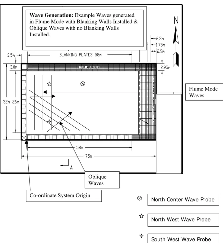
generated in the OEB using standard procedures described in Reference 2. To measure the wave field during testing, IOT would typically install a number of stationary capacitance wave probes at known positions in the OEB co-ordinate system as shown in Figure 3. IOT often tailors model test programs for clients/ collaborators involved in validating time domain numerical prediction software. For these projects, providing time domain wave information at some defined point on the model (typically the model’s center of gravity) is a common
requirement. GEDAP programs ‘WAVETRAN’ or ‘BOAT_WAVE’ can, using data from a stationary wave probe as an input, be used to estimate the variation in wave height at a stationary or moving model subjected to a unidirectional regular or irregular wave field. This document has been written to validate the software, establish boundaries for acceptable output and provide IOT clients/collaborators with some confidence in the integrity of the results generated.
These programs do not provide acceptable results in multi-directional or non-linear waves. Poor results are noted when the generated waves are steep enough to break or where there is a measurable variation in wave celerity as the waves propagate the length of the tank.
3.0 DESCRIPTION OF THE OFFSHORE ENGINEERING BASIN
The IOT Offshore Engineering Basin (OEB) has a working area of 26 m by 65.8 m with a depth that can be varied from 0.1 m to 3.0 m. The depth used for the validation exercise described in this report was 2.8 m. Waves are generated
using 168 individual, computer controlled wet back wavemaker segments, hydraulically activated, fitted around the perimeter of the tank in an “L” configuration. Each segment can be operated in one of three modes of
articulation: flapper mode (± 15º), piston mode (± 400 mm) or a combination of both modes. The wavemakers are capable of generating both regular and
irregular waves up to 0.5 m significant wave height. Passive wave absorbers are fitted around the other two sides of the tank. The facility has a recirculating water system based current generation capability with current speed dependent on water depth, extensive video coverage and is serviced over its entire working area by a 5 t lift capacity crane. Additional information on the OEB can be found in Appendix A.
4.0 DESCRIPTION OF GEDAP PROGRAMS ‘WAVETRAN’ AND ‘BOAT_WAVE’
Both ‘WAVETRAN’ and ‘BOAT_WAVE’ were designed to be used by the GEDAP data analysis software package described in Reference 3. A brief description of the GEDAP software package and documentation on all GEDAP programs available to the IOT user can be found on the IOT internal web site.
‘BOAT_WAVE’ reads in a GEDAP V1 file containing Eta1(t) where Eta1(t) is the wave elevation record of a unidirectional regular or irregular wave train at the position (x1, y1) of a stationary wave probe. At each time step,
‘BOAT_WAVE’ calculates the wave elevation at a desired point on the physical model, specified by two planar position input files X_LOC(t) and Y_LOC(t) normally measured using the QUALISYS optical tracking system described in Reference 4 with additional information presented in Appendix B. Note the QUALISYS infrared (IR) markers on the ship model shown in Figure 1. The wave elevation time series at the desired point on the model is stored in an output file.
‘WAVETRAN’ reads in a GEDAP V1 file containing Eta1(t) where Eta1(t) is the wave elevation record of a unidirectional regular or irregular wave train at the position of a stationary wave probe (x1, y1). At each time step,
‘WAVETRAN’ then calculates the corresponding wave elevation record Eta2(t) at some other defined stationary point (x2, y2) and stores this time series in an output file. Note the array of wave probes around the platform in Figure 2. For both programs, the user specifies the direction of propagation of the unidirectional wave train and the water depth. In addition, both programs use FFT techniques to compute the phase shift of each frequency component on the basis of linear wave theory. The wave direction and planar position in the OEB must be specified in a co-ordinate system defined as follows (see Figure 3):
• origin at the south west corner of the tank. • X co-ordinate positive east
LM-2004-14
• Y co-ordinate positive north
WARNING
: If the planar position data acquired from QUALISYS is
not provided in this co-ordinate system, GEDAP program
‘TRANSFORM1’ must be run to perform a co-ordinate transformation
before using ‘WAVETRAN’ or ‘BOAT_WAVE’. Also the positions of
the wave probes must also be input by the user in this co-ordinate
system.
If there is a tilt to any of the wave probes, this can result in significant
probe position errors. For example, for a water depth of 2.8 m, it will
only require a 4 degree tilt in a wave probe to get a 0.2 m error in
position.
5.0 OEB TEST CONFIGURATIONS
The software was validated using available data acquired during a number of projects carried out over the last few years in the OEB. The following
experiments were carried out: Data Set 1 – Project 977:
Data from three wave probes were acquired for most of the experiments in Data Set 1. A ship model was operating in the tank with planar (X, Y) position
measured using QUALISYS during each run. The co-ordinates of each wave probe are provided as follows:
South West Probe (SW1): X = 15.347 m, Y = 5.775 m North West Probe (NW1): X = 15.230 m, Y = 20.828 m North Center Probe (NC1): X = 29.413 m, Y = 20.837 m See Figure 3 for layout of OEB for Data Set 1.
Wave Configurations - Data Set 1: Regular Waves:
Flume Mode, west wavemakers used only, blanking plates Installed covering north beaches – nominal wave period = 1.12 s to 3.628 s, wave height = 0.0735 m to 0.5 m.
Oblique Waves, west and south wavemakers used, waves generated 60 degrees relative to west wall, no blanking plates installed – nominal wave period = 1.12 s to 3.023 s, wave height = 0.0735 m to 0.5 m.
Irregular Waves:
Flume Mode, west wavemakers used only, blanking plates installed covering north beaches – nominal modal period = 2.6 s, nominal significant wave height = 0.283 m – multiple wave segments were used to cover spectrum. North west wave probe data unavailable.
Oblique Waves, west and south wavemakers used, waves generated 60 degrees relative to west wall, no blanking plates installed – nominal modal period = 2.6 s, nominal significant wave height = 0.283 m – multiple wave segments were used to cover the spectrum.
See Tables 1 - 3 for list of Data Set 1 waves. Data Set 2 – Project 903:
Data from three wave probes were acquired for most of the experiments in Data Set 2. There was no physical model in the tank during these experiments. The co-ordinates of each wave probe are provided as follows:
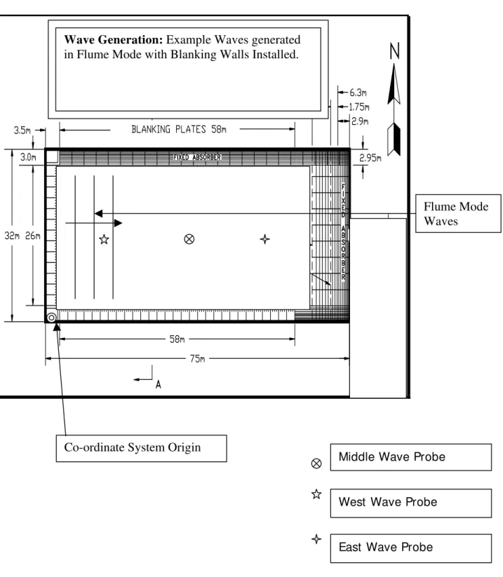
East Probe (EW1): X = 43.541 m, Y = 13.285 m West Probe (WW1): X = 15.005 m, Y = 13.340 m Middle Probe (MW1): X = 29.373 m, Y = 13.330 m See Figure 4 for layout of OEB for Data Set 2. Wave Configurations - Data Set 2:
Regular Waves:
Flume Mode, west wavemakers used only, blanking plates Installed covering north beaches – nominal wave period = 1.43 s to 6.67 s, wave height = 0.05 m to 0.7 m.
Irregular Waves:
Flume Mode, west wavemakers used only, blanking plates installed covering north beaches – nominal mean period = 1.43 to 2.5 s, nominal significant wave height = 0.05 m to 0.6 m – one wave segment from each wave reviewed. See Table 4, 5 for list of Data Set 2 waves.
LM-2004-14
6.0 ‘WAVETRAN’ VALIDATION
The data analysis procedure and the results of the validation of program ‘WAVETRAN’ is presented in this section. For Data Set 1, waves measured using the North West and South West probes were moved to the North Center probe position and compared to waves measured using the North Center probe. For Data Set 2, waves measured using the East and West probes were moved to the Middle probe position and compared to waves measured using the Middle probe. All data acquired in the OEB is initially formatted as GDAC test data acquisition files described in References 5, 6.
Data Analysis Procedure
The following basic data analysis sequence was followed:
• Run GEDAP Program ‘SPLIT_DAC’ to split GDAC test data acquisition files acquired during experiments in the OEB into separate GEDAP format wave data files in model scale units.
• Run GEDAP program ‘WAVETRAN’ to move wave data from one probe position to a second wave probe position. The user inputs the X, Y
position of each wave probe in the specified OEB co-ordinate system with the origin defined at the south west corner of the tank, the water depth (m) and the wave direction with respect to the west tank wall (degrees). • Use GEDAP Program ‘GPLOT’ to review the wave data from all wave
probes in the time domain to determine an acceptable common time segment.
• Run GEDAP Program ‘SELECT1’ to select a common time segment that includes valid data for all wave probes of interest.
• Run GEDAP Program ‘XCORR’ to carry out a cross-correlation between all wave channel time series signals.
• Run GEDAP Program ‘ZCA’ to determine the average wave height, period (HAV, TAV) for regular waves and average as well as maximum wave
height, period (HMAX, TMAX) for irregular waves by carrying out a time
domain zero crossing analysis on the wave time series signals.
• Run GEDAP Program ‘WAVE’ to estimate the breaking wave height given a user specified wave period (s) and water depth (m). (Regular waves only).
Cross-Correlation of two wave signals:
Program ‘XCORR’ computes Rxy(τ) where Rxy(τ) is the cross-correlation
function of two input time series signals, x(t) and y(t). It then locates the value of τ (tau), the time shift in seconds between the two input time series signals, at which the maximum value of Rxy(τ) occurs and applies this time shift to y(t) to obtain a new signal called ys(t). This time-shifted signal ys(t) has maximum correlation with the first input signal, x(t).
The cross-correlation function Rxy(τ) is defined as follows:
Rxy(τ) = Cxy(τ) / (sigma_x * sigma_y)
where Cxy(τ) = the cross-covariance function of x(t) and y(t), sigma_x = the standard deviation of x(t)
and sigma_y = the standard deviation of y(t).
If the two input signals are identical, Rxy(τ) has a maximum value of 1.0 at τ = zero seconds. The cross-covariance function Cxy(τ) is defined by:
Cxy(τ) = E[(x(t) - mux) * (y(t + τ) - muy)]
where E[z] = the expected value of z, mux = mean value of x(t), and muy = mean value of y(t).
Cxy(τ) is computed by an FFT technique which is typically 50 to 100 times faster than calculating Cxy(τ) directly in the time domain. If time shift τ has a negative value, then y(t) leads x(t).
The results of the cross-correlation and zero crossing analysis are presented in Appendix C for the regular waves and Appendix D for the irregular waves.
The criterion for an unacceptable wave signal transfer has been defined as: [τ/TAV] * 100% > 10%
Evaluating the Validation Envelope for ‘WAVETRAN’:
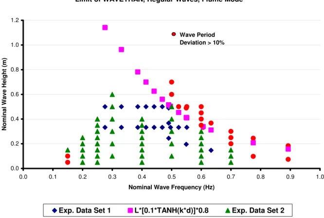
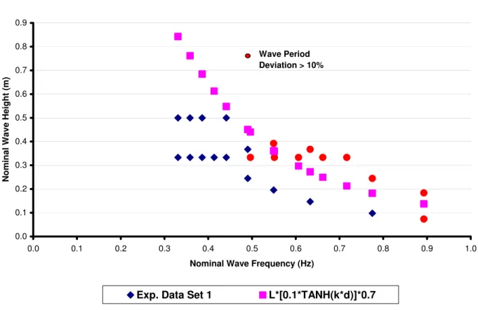
An effort was made to define a safe operating envelope for ‘WAVETRAN’ using the available data. Plots of Nominal Wave Height (m) vs. Nominal Wave
Frequency (Hz) are provided in Figure 5 (regular waves, flume mode), and
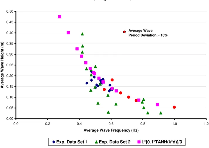
Figure 6 (regular oblique waves). Plots of Average Wave Height (m) vs. Average Wave Frequency (Hz) are presented in Figure 7 (irregular waves, flume mode) and Figure 8 (irregular oblique waves).
The maximum limit for using ‘WAVETRAN’ is defined by the relationship: Lw(0.1*TANH(k * d))*A
Where: Lw = wave length (m) = (2 * π)/(g * Tw2)
g = acceleration due to gravity = 9.808 m/s2 π = 3.14159
LM-2004-14
Tw = wave period (s)
k = wave number (m-1) = (4 * π2)/(g * Tw2)
d = water depth (m) A = constant
= 0.8 for regular waves, flume mode = 0.7 for regular oblique waves
= 1/3 for all irregular waves
The values that exceed the unacceptable criterion are defined by red dots in Figures 5 to 8.
Example Time Series Plots:
The following comparative time series plots are provided: Figure 9: Linear, Regular Wave, Flume Mode
Figure 10: Non-Linear, Regular Wave, Flume Mode Figure 11: Linear, Irregular Wave, Flume Mode Figure 12: Non-Linear, Irregular Wave, Flume Mode Figure 13: Linear, Regular Oblique Wave
Figure 14: Non-Linear, Regular Oblique Wave Example Spectral Density Plots:
A variance spectral density analysis was carried out on both a linear as well as non-linear irregular wave to determine whether using ‘WAVETRAN’ had any significant impact on the spectral characteristics.
Figure 15: Linear Irregular Wave Figure 16: Non-Linear Irregular Wave
A comparison of the spectral parameters for each wave probe is listed in Table 6. Repeatability Check:
The analysis was carried out on six runs that were repeated during the testing. The results of this analysis are provided in Table 7.
7.0 ‘BOAT_WAVE’ VALIDATION
The validation procedure for ‘BOAT_WAVE’ was very similar to the procedure adopted for ‘WAVETRAN’. Only data from Data Set 1 was used to validate this software as there was no moving model in the tank during Data Set 2 project #903.
Data Analysis Procedure
The following basic data analysis sequence was followed:
• Run GEDAP Program ‘SPLIT_DAC’ to split GDAC test data acquisition files acquired during experiments in the OEB into separate GEDAP format wave data files in model scale units.
• Use GEDAP program GPLOT to view the QUALISYS two planar position channels and manually remove any spikes or other unwanted anomalies using GEDAP program DESPIKE or glitch fixing by linear interpolation (GFL) available within GPLOT.
• Run GEDAP program ‘BOAT_WAVE’ to move wave data from the three wave probe positions to the center of gravity of the moving model as measured using QUALISYS. The user inputs the X, Y position of each wave probe in the specified OEB co-ordinate system with the origin defined at the south west corner of the tank, the water depth (m) and the wave direction with respect to the west tank wall (degrees). It was also important to verify that the QUALISYS planar position data was also specified in the OEB co-ordinate system with the origin defined at the south west corner of the tank.
• Use GEDAP Program ‘GPLOT’ to review the wave data from all wave probes in the time domain to determine an acceptable common time segment.
• Run GEDAP Program ‘SELECT1’ to select a common time segment that includes valid data for all wave probes of interest.
• Run GEDAP Program ‘XCORR’ as described in Section 6.0 to carry out a cross-correlation between all three wave channel time series signals at the center of gravity of the model.
WARNING
: If the position of the model as measured using
QUALISYS is not carefully despiked, these unwanted anomalies will be
reflected in the wave data moved to the model.
Since ‘BOAT_WAVE’ is essentially based on the same principals as
‘WAVETRAN’, it is assumed that the valid operating envelope for ‘BOAT_WAVE’ matches the valid operating envelope for ‘WAVETRAN’ and the same user restrictions apply. To verify this assumption, a small random subset of runs from Data Set 1 were evaluated using the same criterion ([τ/TAV] * 100% > 10%) as
was used for ‘WAVETRAN’. The results of the regular wave analysis for flume mode and oblique waves are presented in Table 8 while the irregular wave analysis for flume mode and oblique waves is presented in Table 9.
LM-2004-14
8.0 DISCUSSION
The primary objective of the validation exercise was to determine if the software provided satisfactory results relative to a defined criterion and attempt to define the boundaries of acceptable performance. The two wave data sets used to achieve these goals were not dedicated to validating this software so there are some limitations.
8.1 ‘WAVETRAN’ Validation Results
Referring to plots defining the envelope for valid use of ‘WAVETRAN’ (Figures 5 – 8):
Other than for the regular wave, flume mode (Figure 5), there is not enough data to fully define the envelope for valid use however the following observations can be made:
Regular Waves, Flume Mode (Figure 5): There is enough data available for this situation to make definitive conclusions with respect to the performance of the software. There is little scatter in the data and the invalid results can be
expected for wave height and frequency combinations that exceed a line defined by Lw(0.1*TANH(k * d))*0.8. Also, due to scatter at very low wave amplitudes,
the software is not deemed to be reliable at wave heights less than 10 cm. Regular Oblique Waves (Figure 6): Even though there is a smaller data set available, it is apparent that there is more scatter and less reliability when using ‘WAVETRAN’ in oblique seas. Generally invalid results can be expected for wave height and frequency combinations that exceed a line defined by
Lw(0.1*TANH(k * d))*0.7. Also, due to scatter at very low wave amplitudes, the
software is not deemed to be reliable at wave heights less than 10 cm. Irregular Waves, Flume Mode (Figure 7): The envelope for valid use of
‘WAVETRAN’ is more complex in irregular seas. Generally invalid results can be expected for average wave height and frequency combinations that exceed a line defined by Lw(0.1*TANH(k * d))/3 - for average wave heights less than 0.25 m.
For average wave heights greater than 0.25 m, there appears to be more stability in the results. This is probably due to the fact that an average wave height and frequency is being used and although individual waves in the irregular wave time series may be breaking; it doesn’t appear to have a major impact on the average wave height or frequency of the wave train.
Irregular Oblique Waves (Figure 8): There is insufficient irregular oblique wave data available to fully define an envelope for valid use of ‘WAVETRAN’ however the data implies that generally invalid results can be expected for average wave height and frequency combinations that exceed a line defined by Lw(0.1*TANH(k
* d))/3. It is safe to say however, that some scatter can be expected in the results and caution must be exercised in using ‘WAVETRAN’ in this situation. Generally the results using ‘WAVETRAN’ for regular waves with the OEB in flume mode are the best. Figure 9 illustrates a typical time series plot and demonstrates that there is little phase shift or deviation in wave height.
Figure 10 illustrates what happens if a regular wave breaks between the time it is measured using the two west wave probes and when it reaches the north center wave probe. There is an unacceptable phase shift although there does not appear to be a major impact on wave height.
There is fairly a consistent correlation between the outputs of the three wave probes when measuring linear irregular waves with the tank in flume mode (Figure 11). The phase relationship comparison is very good however there is some variation in wave height noted.
There does not appear to be any correlation between the wave probe signals for the non-linear irregular wave illustrated in Figure12. It is clear that ‘WAVETRAN’ gives unacceptable results in this situation.
Figure 13 and 14 provide an example of the difference in phase relationship that can be expected after transferring a linear and non-linear regular oblique wave. Note the lower wave amplitude for the north west probe in Figure 13. This probe is located close to the corner in the tank where the west wave board bank and north beach meet. It is possible that the location of the north west probe may result in some local distortion here since the data from the south west probe looks fine. Figure 14 illustrates the impact on phase when waves break between wave probe locations.
An example comparison of the spectral characteristics between the wave probes was investigated for a linear (Data Set 2: File IR_010_001) and non-linear (Data Set 2: File IR_018_001) irregular wave case in Figures 15, 16, and Table 6. The fact that there are relatively small differences between the spectra for each wave probe - even for the non-linear waves (little difference in spectral shape,
amplitude, spectral peak) implies that the overall characteristics do not change significantly. Thus there is likely a phase shift in the time series of the non-linear wave but little alteration in the spectral characteristics.
8.2 ‘BOAT_WAVE’ Validation Results
Referring to Tables 8, 9 and comparing the results with the results for the same runs from ‘WAVETRAN’ presented in Appendix C and D, it is apparent that the same trends exist and thus it can be assumed that the valid envelope defined for ‘WAVETRAN’ can be adopted for ‘BOAT_WAVE’.
LM-2004-14
9.0 CONCLUSIONS AND RECOMMENDATIONS
Based on the data sets analyzed, the following recommendations and restrictions for using ‘WAVETRAN’ and ‘BOAT_WAVE’ are provided in this section:
9.1 Programs ‘WAVETRAN’ and ‘BOAT_WAVE’
• Satisfactory results can be derived using ‘WAVETRAN’ and
‘BOAT_WAVE’ to analyze regular waves with the OEB in flume mode for wave height and frequency combinations not exceeding a line defined by Lw(0.1*TANH(k * d))*0.8 and the wave heights greater than 10 cm.
• Satisfactory results can be derived using ‘WAVETRAN’ and
‘BOAT_WAVE’ to analyze regular oblique waves with the OEB for wave height and frequency combinations not exceeding a line defined by Lw(0.1*TANH(k * d))*0.7 and the wave heights greater than 10 cm.
• Satisfactory results can be derived using ‘WAVETRAN’ and
‘BOAT_WAVE’ to analyze irregular waves with the OEB in flume mode for average wave height and frequency combinations not exceeding a line defined by Lw(0.1*TANH(k * d))/3 - for average wave heights less than
0.25 m although caution should be exercised by the user since more data is required to further validate the software.
• Satisfactory results can be derived using ‘WAVETRAN’ and
‘BOAT_WAVE’ to analyze irregular oblique waves with the OEB for wave height and frequency combinations not exceeding a line defined by
Lw(0.1*TANH(k * d))/3 although caution must be exercised as the data set
analyzed was too small to fully define a valid operating envelope. • ‘WAVETRAN’ and ‘BOAT_WAVE’ work best in regular waves with the
OEB in flume mode however scatter can be expected in the integrity of the results for oblique and/or irregular waves.
• The location of the wave probes appears to have an influence of the integrity of the results using ‘WAVETRAN’. It is recommended that ‘WAVETRAN’ not be used to transfer data from a wave probe positioned close to wave boards or beaches in oblique waves.
• There is little variation in the irregular wave spectral characteristics between wave probes after ‘WAVETRAN’ has been used to transfer the wave data from one point to another – even for non-linear waves. • Good repeatability has been demonstrated.
9.2 Other Recommendations
• Additional data is required to fully validate these programs – especially in oblique irregular seas.
• Only wave data acquired in the OEB has been used in this document. A separate exercise should be carried out to derive/validate software to move wave data from a wave probe fitted at one end of the IOT tow tank carriage to a specified point on a free-running model free to surge.
10.0 ACKNOWLEDGEMENTS
The authors would like to thank Dr. E. Baddour for permission to use wave data from Project #903 in assist with the validation of this software.
11.0 REFERENCES
1) Institute for Ocean Technology Standard Test Method: Seakeeping, V1.0, 42-8595-S/GM-5, November 15, 2001.
2) Institute for Ocean Technology Standard Test Method: Environmental Modeling – Waves, Wind, Current, V4.0, 42-8595-S/GM-3, January 3, 2002.
3) Miles, M.D.,”The GEDAP Data Analysis Software Package”, NRC Institute for Mechanical Engineering, Hydraulics Laboratory Report No. TR-HY-030, August 11, 1990.
4) Sullivan, M., “Optical Tracking at the Institute for Marine Dynamics”, Proc. of the 4th Canadian Marine Hydrodynamics and Structures Conference, Ottawa, June 23 – 25, 1997, IMD Report #IR-1997-15, July 1997. 5) Miles, M.D.,”Test Data File for New GDAC Software”, NRC Institute for
Marine Dynamics Software Design Specification, Version 3.0, January 2, 1996.
6) Miles, M.D.,”DACON Configuration File for New GDAC Software”, NRC Institute for Marine Dynamics Software Design Specification, Version 3.2, August 14, 1996.
LE 1: DATA SET 1 – REGULAR WAVES, FLUME MODE
Validation of GEDAP Program 'WAVETRAN' & 'BOAT_WAVE' - DATA SET 1
Regular Waves - Flume Mode:
Est. Wave Breaking T1 T2 Wave Period Wave Frequency Wave Height Wave Height
Filename (s) (s) (s) (Hz) (m) (m)
NOTE: OEB in Flume Mode (waves generated 0 deg. from west wall), blanking walls installed covering all north beaches.
FS8_180HG_0HG_0p75WL_0p04WS_002 60 80 1.12 0.8929 0.0735 0.19578 FS8_180HG_0HG_0p75WL_0p1WS_001 60 80 1.12 0.8929 0.1838 0.19578 FS8_180HG_0HG_1p0WL_0p04WS_001 50 70 1.29 0.7752 0.0980 0.25973 FS8_0HG_1p0WL_0p1WS_001 45 65 1.29 0.7752 0.2450 0.25973 FS8_180HG_0HG_1p5WL_0p04WS_001 40 60 1.58 0.6329 0.1470 0.38945 FS8_0HG_1p5WL_0p1WS_001 35 55 1.58 0.6329 0.3675 0.38945 test_011 40 60 1.649 0.6064 0.3330 0.42398 test_008 40 60 1.814 0.5513 0.3330 0.51145 test_132 35 55 1.814 0.5513 0.5000 0.51145 FS13_180HG_0HG_2p0WL_0p04WS_001 60 80 1.82 0.5495 0.1960 0.51474 FS13_0HG_2p0WL_0p1WS_001 52 70 1.82 0.5495 0.4900 0.51474 test_141 35 55 1.909 0.5238 0.3330 0.56424 test_153 32 52 1.909 0.5238 0.5000 0.56424 test_140 35 55 2.015 0.4963 0.3330 0.62435 test_154 30 50 2.015 0.4963 0.5000 0.62435 FS8_180HG_0HG_2p5WL_0p04WS_001 40 70 2.04 0.4902 0.2450 0.63861 FS0_180HG_2p5WL_0p06WS_001 60 90 2.04 0.4902 0.3675 0.63861 FS8_0HG_2p5WL_0p08WS_001 28 45 2.04 0.4902 0.4900 0.63861 test_139 35 60 2.134 0.4686 0.3330 0.69217 test_150 30 49 2.134 0.4686 0.5000 0.69217 test_138 40 60 2.267 0.4411 0.3330 0.7668 test_149 32 52 2.267 0.4411 0.5000 0.7668 test_137 35 55 2.418 0.4136 0.3330 0.84805 test_148 30 50 2.418 0.4136 0.5000 0.84805 test_136 35 55 2.591 0.3860 0.3330 0.93463 test_147 35 60 2.591 0.3860 0.5000 0.93463 test_135 32 56 3.023 0.3308 0.3330 1.1152 test_146 35 60 3.023 0.3308 0.5000 1.1152 test_134 30 55 3.628 0.2756 0.3330 1.2922 test_145 35 60 3.628 0.2756 0.5000 1.2922 NOTE:
Wave height, wave period and wave direction are nominal values.
Estimated breaking wave height computed for user input water depth and wave period (computed using GEDAP Program 'WAVE') T1, T2 - Start, End Segment Select Time
TAB
LM-2004-14
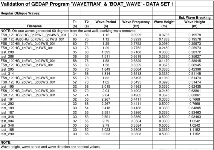
Validation of GEDAP Program 'WAVETRAN' & 'BOAT_WAVE' - DATA SET 1 Regular Oblique Waves:
Est. Wave Breaking T1 T2 Wave Period Wave Frequency Wave Height Wave Height
Filename (s) (s) (s) (Hz) (m) (m)
NOTE: Oblique waves generated 60 degrees from the west wall, blanking walls removed.
FS8_120HG60HG_0p75WL_0p04WS_001 70 88 1.12 0.8929 0.0735 0.19578 FS8_120HG60HG_0p75WL_0p1WS_001 65 75 1.12 0.8929 0.1838 0.19578 FS8_120HG_1p0WL_0p04WS_001 60 74 1.29 0.7752 0.0980 0.25973 FS8_120HG_1p0WL_0p1WS_001 60 76 1.29 0.7752 0.2450 0.25973 test_289 35 60 1.395 0.7168 0.3330 0.30372 test_288 36 56 1.511 0.6618 0.3330 0.35627 FS8_120HG_1p5WL_0p04WS_001 58 76 1.58 0.6329 0.1470 0.38945 FS8_120HG_1p5WL_0p1WS_001 55 80 1.58 0.6329 0.3675 0.38945 test_285 35 70 1.649 0.6064 0.3330 0.42398 test_314 34 56 1.814 0.5513 0.3330 0.51145 FS8_120HG_2p0WL_0p04WS_001 55 78 1.82 0.5495 0.1960 0.51474 FS8_120HG_2p0WL_0p08WS_001 52 78 1.82 0.5495 0.3920 0.51474 test_195 32 58 2.015 0.4963 0.3330 0.62435 FS8_120HG_2p5WL_0p04WS_001 52 70 2.04 0.4902 0.2450 0.63861 FS8_120HG_2p5WL_0p06WS_001 52 74 2.04 0.4902 0.3675 0.63861 test_191 32 55 2.267 0.4411 0.3330 0.7668 test_292 32 68 2.267 0.4411 0.5000 0.7668 test_189 30 54 2.418 0.4136 0.3330 0.84805 test_187 32 55 2.591 0.3860 0.3330 0.93463 test_348 30 53 2.591 0.3860 0.5000 0.93463 test_304 32 55 2.79 0.3584 0.3330 1.0242 test_346 30 53 2.79 0.3584 0.5000 1.0242 test_185 30 52 3.023 0.3308 0.3330 1.1152 test_290 30 65 3.023 0.3308 0.5000 1.1152 NOTE:
Wave height, wave period and wave direction are nominal values.
Estimated breaking wave height computed for user input water depth and wave period (computed using GEDAP Program 'WAVE') T1, T2 - Start, End Segment Select Time
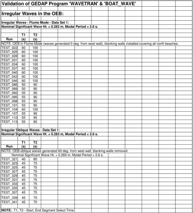
Validation of GEDAP Program 'WAVETRAN' & 'BOAT_WAVE' Irregular Waves in the OEB:
Irregular Waves - Flume Mode - Data Set 1:
Nominal Significant Wave Ht. = 0.283 m, Modal Period = 2.6 s.
T1 T2 Run (s) (s)
NOTE: OEB in Flume Mode (waves generated 0 deg. from west wall), blanking walls installed covering all north beaches. TEST_022 60 100 TEST_025 60 100 TEST_028 60 100 TEST_031 60 100 TEST_034 60 100 TEST_037 60 100 TEST_040 60 100 TEST_043 60 100 TEST_046 60 100 TEST_086 50 90 TEST_089 50 90 TEST_092 55 95 TEST_095 55 95 TEST_098 55 95 TEST_101 55 95 TEST_104 60 100 TEST_107 55 95 TEST_110 55 95 TEST_113 55 95
Irregular Oblique Waves - Data Set 1:
Nominal Significant Wave Ht. = 0.283 m, Modal Period = 2.6 s.
T1 T2 Run (s) (s)
NOTE: OEB oblique waves generated 60 deg. from west wall, blanking walls removed. Nominal Significant Wave Ht. = 0.283 m, Modal Period = 2.6 s.
TEST_321 40 80 TEST_323 45 75 TEST_325 45 75 TEST_327 45 75 TEST_329 45 75 TEST_331 45 75 TEST_333 45 75 TEST_335 45 75 TEST_337 45 75 TEST_339 45 75 TEST_341 45 75
NOTE: T1, T2 - Start, End Segment Select Time
The wave spectrum was divided into a number of components - each test is a different segment.
LM-2004-14
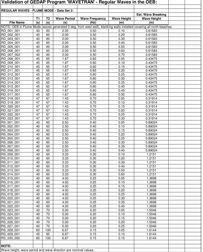
Validation of GEDAP Program 'WAVETRAN' - Regular Waves in the OEB:
REGULAR WAVES - FLUME MODE - Data Set 2:
Est. Wave Breaking T1 T2 Wave Period Wave Frequency Wave Height Wave Height File Name (s) (s) (s) (Hz) (m) (m)
NOTE: OEB in Flume Mode (waves generated 0 deg. from west wall), blanking walls installed covering all north beaches.
RD_001_001 40 60 2.00 0.50 0.10 0.61583 RD_002_001 40 60 2.00 0.50 0.20 0.61583 RD_003_001 40 60 2.00 0.50 0.30 0.61583 RD_004_001 40 60 2.00 0.50 0.40 0.61583 RD_005_001 40 60 2.00 0.50 0.50 0.61583 RD_006_001 40 60 2.00 0.50 0.60 0.61583 RD_007_002 40 60 2.00 0.50 0.70 0.61583 RD_008_001 45 65 1.67 0.60 0.05 0.43475 RD_009_001 45 65 1.67 0.60 0.10 0.43475 RD_010_001 45 65 1.67 0.60 0.15 0.43475 RD_011_001 45 65 1.67 0.60 0.20 0.43475 RD_012_001 45 65 1.67 0.60 0.25 0.43475 RD_013_001 45 65 1.67 0.60 0.30 0.43475 RD_014_001 45 65 1.67 0.60 0.35 0.43475 RD_015_001 45 65 1.67 0.60 0.40 0.43475 RD_016_001 45 65 1.67 0.60 0.45 0.43475 RD_017_001 45 65 1.67 0.60 0.50 0.43475 RD_018_001 47 67 1.43 0.70 0.05 0.31914 RD_019_001 47 67 1.43 0.70 0.10 0.31914 RD_020_001 47 67 1.43 0.70 0.15 0.31914 RD_021_001 47 67 1.43 0.70 0.20 0.31914 RD_022_001 47 67 1.43 0.70 0.25 0.31914 RD_023_001 47 67 1.43 0.70 0.30 0.31914 RS_001_001 40 60 2.50 0.40 0.05 0.89024 RS_002_001 40 60 2.50 0.40 0.10 0.89024 RS_003_001 40 60 2.50 0.40 0.15 0.89024 RS_004_001 40 60 2.50 0.40 0.20 0.89024 RS_005_001 40 60 2.50 0.40 0.25 0.89024 RS_006_001 40 60 2.50 0.40 0.30 0.89024 RS_007_001 40 60 2.50 0.40 0.35 0.89024 RS_008_001 40 60 2.50 0.40 0.40 0.89024 RS_009_001 40 60 3.33 0.30 0.10 1.2151 RS_010_001 40 60 3.33 0.30 0.20 1.2151 RS_011_001 40 60 3.33 0.30 0.30 1.2151 RS_012_001 40 60 3.33 0.30 0.40 1.2151 RS_013_001 40 60 3.33 0.30 0.50 1.2151 RS_014_001 40 60 3.33 0.30 0.60 1.2151 RS_015_001 40 60 4.00 0.25 0.05 1.3698 RS_016_001 40 60 4.00 0.25 0.10 1.3698 RS_017_001 40 60 4.00 0.25 0.15 1.3698 RS_018_001 40 60 4.00 0.25 0.20 1.3698 RS_019_001 40 60 4.00 0.25 0.25 1.3698 RS_020_001 40 60 4.00 0.25 0.30 1.3698 RS_021_001 40 60 4.00 0.25 0.35 1.3698 RS_022_001 40 60 4.00 0.25 0.40 1.3698 RS_023_001 40 70 5.00 0.20 0.05 1.5046 RS_024_001 40 70 5.00 0.20 0.10 1.5046 RS_025_001 40 70 5.00 0.20 0.15 1.5046 RS_026_001 40 70 5.00 0.20 0.20 1.5046 RS_027_001 40 70 5.00 0.20 0.25 1.5046 RS_028_001 60 100 6.67 0.15 0.05 1.6144 RS_029_001 45 85 6.67 0.15 0.10 1.6144 RS_030_002 60 100 6.67 0.15 0.15 1.6144 NOTE:
Wave height, wave period and wave direction are nominal values.
Estimated breaking wave height computed for user input water depth and wave period (computed using GEDAP Program 'WAVE') T1, T2 - Start, End Segment Select Time
TABLE 4: DATA SET 2 – REGULAR WAVES, FLUME MODE
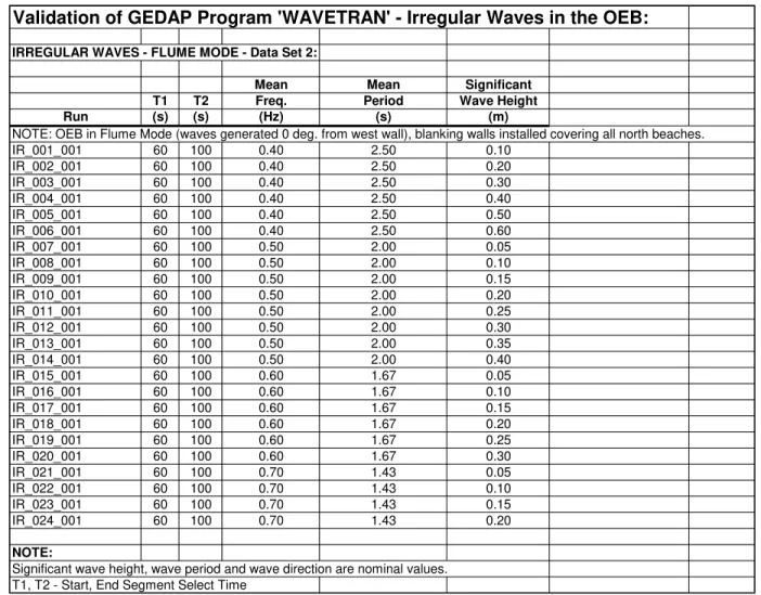
A SET 2 – IRREGULAR FLUME MODE WAVES
Validation of GEDAP Program 'WAVETRAN' - Irregular Waves in the OEB: IRREGULAR WAVES - FLUME MODE - Data Set 2:
Mean Mean Significant T1 T2 Freq. Period Wave Height
Run (s) (s) (Hz) (s) (m)
NOTE: OEB in Flume Mode (waves generated 0 deg. from west wall), blanking walls installed covering all north beaches.
IR_001_001 60 100 0.40 2.50 0.10 IR_002_001 60 100 0.40 2.50 0.20 IR_003_001 60 100 0.40 2.50 0.30 IR_004_001 60 100 0.40 2.50 0.40 IR_005_001 60 100 0.40 2.50 0.50 IR_006_001 60 100 0.40 2.50 0.60 IR_007_001 60 100 0.50 2.00 0.05 IR_008_001 60 100 0.50 2.00 0.10 IR_009_001 60 100 0.50 2.00 0.15 IR_010_001 60 100 0.50 2.00 0.20 IR_011_001 60 100 0.50 2.00 0.25 IR_012_001 60 100 0.50 2.00 0.30 IR_013_001 60 100 0.50 2.00 0.35 IR_014_001 60 100 0.50 2.00 0.40 IR_015_001 60 100 0.60 1.67 0.05 IR_016_001 60 100 0.60 1.67 0.10 IR_017_001 60 100 0.60 1.67 0.15 IR_018_001 60 100 0.60 1.67 0.20 IR_019_001 60 100 0.60 1.67 0.25 IR_020_001 60 100 0.60 1.67 0.30 IR_021_001 60 100 0.70 1.43 0.05 IR_022_001 60 100 0.70 1.43 0.10 IR_023_001 60 100 0.70 1.43 0.15 IR_024_001 60 100 0.70 1.43 0.20 NOTE:
Significant wave height, wave period and wave direction are nominal values. T1, T2 - Start, End Segment Select Time
LM-2004-14
File: IR_010_001 LINEAR IRREGULAR WAVE
Wave Probe WW1 Frequency of Spectral Peak (Hz) 0.52500 Wave Probe WW1 Period of Spectral Peak (s) 1.9048 Wave Probe WW1 Significant Wave Height Est. (m)* 0.17886 Wave Probe MW1 Frequency of Spectral Peak (Hz) 0.52497 Wave Probe MW1 Period of Spectral Peak (s) 1.9049 Wave Probe MW1 Significant Wave Height Est. (m)* 0.18184 Wave Probe EW1 Frequency of Spectral Peak (Hz) 0.52500 Wave Probe EW1 Period of Spectral Peak (s) 1.9048 Wave Probe EW1 Significant Wave Height Est. (m)* 0.17839 File: IR-018_001 NON-LINEAR IRREGULAR WAVE
Wave Probe WW1 Frequency of Spectral Peak (Hz) 0.54250 Wave Probe WW1 Period of Spectral Peak (s) 1.8433 Wave Probe WW1 Significant Wave Height Est. (m)* 0.18038 Wave Probe MW1 Frequency of Spectral Peak (Hz) 0.54247 Wave Probe MW1 Period of Spectral Peak (s) 1.8434 Wave Probe MW1 Significant Wave Height Est. (m)* 0.18667 Wave Probe EW1 Frequency of Spectral Peak (Hz) 0.52500 Wave Probe EW1 Period of Spectral Peak (s) 1.9048 Wave Probe EW1 Significant Wave Height Est. (m)* 0.17217
* NOTE: Significa rd deviation from th
ABLE 6: COMPARISON OF SPECTRAL PARAMETERS (‘WAVETRAN’) nt wave height estimate = 4 * standa the zero spectral moment (M0) after filtering at lower and upper frequency limit of spectrum.
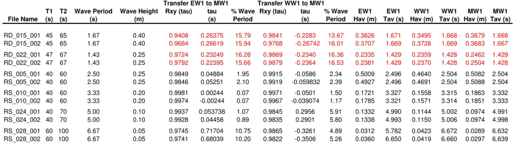
REPEATABILITY CHECK:
Transfer EW1 to MW1 Transfer WW1 to MW1
T1 T2 Wave Period Wave Height Rxy (tau) tau % Wave Rxy (tau) tau % Wave EW1 EW1 WW1 WW1 MW1 MW1
File Name (s) (s) (s) (m) (s) Period (s) Period Hav (m) Tav (s) Hav (m) Tav (s) Hav (m) Tav (s)
RD_015_001 45 65 1.67 0.40 0.9408 0.26375 15.79 0.9841 -0.2283 13.67 0.3626 1.671 0.3495 1.668 0.3679 1.668 0.9684 0.26619 15.94 0.9768 -0.26742 16.01 0.3707 1.669 0.3728 1.669 0.3683 1.667 0.9724 0.23249 16.26 0.9869 -0.2340 16.36 0.2335 1.429 0.2359 1.428 0.2462 1.429 0.9792 0.22395 15.66 0.9879 -0.2364 16.53 0.2381 1.429 0.2370 1.428 0.2504 1.428 RD_015_002 45 65 1.67 0.40 RD_022_001 47 67 1.43 0.25 RD_022_002 47 67 1.43 0.25 RS_005_001 40 60 2.50 0.25 0.9849 0.04884 1.95 0.9915 -0.0586 2.34 0.5009 2.496 0.4640 2.504 0.5082 2.504 RS_005_002 40 60 2.50 0.25 0.9846 0.05251 2.10 0.9919 -0.059832 2.39 0.4927 2.496 0.4691 2.504 0.5088 2.504 RS_010_001 40 60 3.33 0.20 0.9981 0.00244 0.07 0.9971 -0.0501 1.50 0.1721 3.327 0.1558 3.315 0.1863 3.332 RS_010_002 40 60 3.33 0.20 0.9974 -0.00244 0.07 0.9967 -0.039074 1.17 0.1785 3.321 0.1571 3.314 0.1851 3.333 RS_024_001 40 70 5.00 0.10 0.9937 0.053738 1.07 0.9845 0.2956 5.91 0.1332 4.990 0.1144 5.002 0.0974 4.991 RS_024_002 40 70 5.00 0.10 0.9928 0.04458 0.89 0.9835 0.2901 5.80 0.1338 4.993 0.1150 5.006 0.0974 4.998 RS_028_001 60 100 6.67 0.05 0.9745 0.71704 10.75 0.9865 -0.3261 4.89 0.0312 5.782 0.0423 6.672 0.0289 6.632 RS_028_002 60 100 6.67 0.05 0.9741 0.68039 10.20 0.9822 -0.3506 5.26 0.0360 6.650 0.0419 6.660 0.0297 6.639
LM-2004-14
Validation of GEDAP Program 'BOAT_WAVE' - Regular Waves in the OEB:
Regular Waves Data Set 1:
Transfer NW1 to NC1 Transfer SW1 to NC1 Transfer SW1 to NW1 T1 T2 Wave Period Wave Frequency Wave Height Rxy (tau) tau % Wave Rxy (tau) tau % Wave Rxy (tau) tau % Wave Filename (s) (s) (s) (Hz) (m) (s) Period (s) Period (s) Period
NOTE: OEB in Flume Mode (waves generated 0 deg. from west wall), blanking walls installed covering all north beaches.
FS8_180HG_0HG_0p75WL_0p04WS_002 70 95 1.12 0.8929 0.0735 0.9980 -0.0916 8.18 0.9983 -0.0702 6.27 0.9978 0.0214 1.91 FS8_0HG_1p0WL_0p1WS_001 40 70 1.29 0.7752 0.2450 0.8675 -0.5973 46.30 0.8936 -0.4911 38.07 0.9912 0.0989 7.67 0.5495 0.1960 0.9973 -0.0489 2.69 0.9973 -0.0269 1.48 0.9978 0.0196 1.07 0.8929 0.0735 0.9680 -0.06599 5.89 0.9912 -0.16498 14.73 0.9804 -0.0990 8.84 0.7752 0.2450 0.9825 -0.21902 16.98 0.9591 -0.52018 40.32 0.9777 -0.2973 23.04 0.6329 0.3675 0.9799 -0.17714 11.21 0.9610 -0.47035 29.77 0.9828 -0.2902 18.36 0.5495 0.3920 0.9928 -0.14174 7.79 0.9947 -0.23461 12.89 0.9965 -0.0904 4.97 0.4411 0.5000 0.9853 -0.16076 7.09 0.9892 -0.18128 8.00 0.9952 -0.0274 1.21 RED FS13_180HG_0HG_2p0WL_0p04WS_001 60 80 1.82 FS8_180HG_0HG_2p5WL_0p04WS_001 40 70 2.04 0.4902 0.2450 0.9904 -0.0366 1.80 0.9914 -0.0037 0.18 0.9978 0.0330 1.62 test_150 30 49 2.134 0.4686 0.5000 0.9950 -0.1625 7.62 0.9953 -0.1695 7.94 0.9979 -0.0070 0.33 test_148 30 50 2.418 0.4136 0.5000 0.9964 -0.0587 2.43 0.9978 -0.0538 2.22 0.9980 0.0049 0.20 test_134 30 55 3.628 0.2756 0.3330 0.9913 -0.1436 3.96 0.9973 0.1374 3.79 0.9890 0.2810 7.75
Regular Waves - Data Set 1:
Transfer NW1 to NC1 Transfer SW1 to NC1 Transfer SW1 to NW1 T1 T2 Wave Period Wave Frequency Wave Height Rxy (tau) tau % Wave Rxy (tau) tau % Wave Rxy (tau) tau % Wave Filename (s) (s) (s) (Hz) (m) (s) Period (s) Period (s) Period
NOTE: Oblique waves generated 60 degrees from the west wall, blanking walls removed. FS8_120HG60HG_0p75WL_0p04WS_001 70 88 1.12
FS8_120HG_1p0WL_0p1WS_001 60 76 1.29 FS8_120HG_1p5WL_0p1WS_001 55 80 1.58 FS8_120HG_2p0WL_0p08WS_001 52 78 1.82
test_292 32 68 2.267
test_348 30 53 2.591 0.3860 0.5000 N/A N/A N/A 0.9680 -0.06965 2.69 N/A N/A N/A test_185 30 52 3.023 0.3308 0.3330 0.998 0 0.00 0.9958 -0.06354 2.10 0.9958 -0.0611 2.02
NOTE:
Wave height, wave period and wave direction are nominal values.
Estimated breaking wave height computed for user input water depth and wave period.
Rxy (tau) - cross correlation function between two wave probe signals. If two signals are identical, Rxy (tau) = 1.0. tau - time lag (s) between two wave probe signals.
Non-linear Wave is defined as 0.7*H/L < 0.1TANH(kd) (ie: wave is too close to breaking to provide satisfactory solution using WAVETRAN) Where: H = wave height (m)
L = wave length (m) = 2*PI/g*TW2
g = acceleration due to gravity (m/s2) = 9.808 m/s2
PI = 3.14159 TW = wave period (s)
k = wave number (m-1) = (4*PI2)/(g*T W2)
d = water depth (m)
% Wave Period = (tau/nominal wave period) * 100
N/A = Not Available T1, T2 - Start, End Segment Select Time Linear Data in BLACK, Non-linear Data in
Validation of GEDAP Program 'BOAT_WAVE' - Irregular Waves in the OEB:
Data Set 1:Transfer NW1 to NC1 Transfer SW1 to NC1 Transfer SW1 to NW1
T1 T2 Rxy (tau) tau % Wave Rxy (tau) tau % Wave Rxy (tau) tau % Wave
Run (s) (s) (s) Period (s) Period (s) Period
NOTE: OEB in Flume Mode (waves generated 0 deg. from west wall), blanking walls installed covering all north beaches. Nominal Significant Wave Ht. = 0.283 m, Modal Period = 2.6 s.
TEST_025 70 100 0.9665 -0.08062 4.89 0.9390 -0.069626 4.22 0.9884 0.011 0.67
TEST_037 70 100 0.9393 -0.095278 5.09 0.9173 -0.073291 3.91 0.9909 0.018 0.98
TEST_086 50 90 0.9348 -0.004885 0.29 0.9200 0.004885 0.29 0.9856 0.034 2.04
TEST_101 60 95 0.9509 0 0.00 0.9312 0.003665 0.18 0.9861 0.004 0.18
TEST_113 63 80 0.9743 0.039475 2.01 0.9651 0.062329 3.17 0.9890 0.017 0.85
NOTE: % Wave Period has been defined as tau/Average Wave Period @ north center wave probe
Rxy (tau) - cross correlation function between two wave probe signals. If two signals are identical, Rxy (tau) = 1.0. tau - time lag (s) between two wave probe signals. (-ve is lead)
T1, T2 - Start, End Segment Select Time
Data Set 1:
Transfer NW1 to NC1 Transfer SW1 to NC1 Transfer SW1 to NW1
T1 T2 Rxy (tau) tau % Wave Rxy (tau) tau % Wave Rxy (tau) tau % Wave
Run (s) (s) (s) Period (s) Period (s) Period
NOTE: OEB oblique waves generated 60 deg. from west wall, blanking walls removed. Nominal Significant Wave Ht. = 0.283 m, Modal Period = 2.6 s.
TEST_323 40 70 N/A N/A N/A 0.8523 -0.1759 6.61 N/A N/A N/A
TEST_329 40 70 N/A N/A N/A 0.9329 -0.14292 6.62 N/A N/A N/A
TEST_335 40 70 N/A N/A N/A 0.8148 -0.1759 8.98 N/A N/A N/A
TEST_341 40 70 N/A N/A N/A 0.8669 -0.18323 10.43 N/A N/A N/A
Capacitance Wave Probe
QUALISYS Markers
Figure 1: Typical Seakeeping Test on a Ship Model in OEB
LM-2004-14
Wave Generation: Example Waves generated
in Flume Mode with Blanking Walls Installed & Oblique Waves with no Blanking Walls
Installed.
Oblique
Waves Co-ordinate System Origin
North Center Wave Probe Flume Mode Waves
North West Wave Probe
South West Wave Probe
Wave Generation: Example Waves generated in Flume Mode with Blanking Walls Installed.
Middle Wave Probe
Flume Mode Waves
West Wave Probe
East Wave Probe Co-ordinate System Origin
LM-2004-14
Limit of WAVETRAN, Regular Waves, Flume Mode
0.0 0.2 0.4 0.6 0.8 1.0 1.2 0.0 0.1 0.2 0.3 0.4 0.5 0.6 0.7 0.8 0.9 1.0
Nominal Wave Frequency (Hz)
Nominal Wave Height (m)
Exp. Data Set 1 L*[0.1*TANH(k*d)]*0.8 Exp. Data Set 2
Wave Period Deviation > 10%
Limits of WAVETRAN, Regular Oblique Waves 0.0 0.1 0.2 0.3 0.4 0.5 0.6 0.7 0.8 0.9 0.0 0.1 0.2 0.3 0.4 0.5 0.6 0.7 0.8 0.9 1.0
Nominal Wave Frequency (Hz)
Nominal Wave Height (m)
Exp. Data Set 1 L*[0.1*TANH(k*d)]*0.7
Wave Period Deviation > 10%
LM-2004-14
Limits of WAVETRAN, Irregular Waves, Flume Mode
0.00 0.05 0.10 0.15 0.20 0.25 0.30 0.35 0.40 0.45 0.50 0.0 0.2 0.4 0.6 0.8 1.0 1.2
Average Wave Frequency (Hz)
Average Wave Height (m)
Exp. Data Set 1 Exp. Data Set 2 L*[0.1*TANH(k*d)]/3
Average Wave Period Deviation > 10%
Limits of WAVETRAN, Irregular Oblique Seas 0.00 0.05 0.10 0.15 0.20 0.25 0.30 0.35 0.40 0.45 0.50 0.0 0.1 0.2 0.3 0.4 0.5 0.6 0.7 0.8 0.9 1.0
Average Wave Frequency (Hz)
Average Wave Height (m)
Exp. Data Set 1 L*[0.1*TANH(k*d)]/3
Average Wave Period Deviation > 10%
LM-2004-14
LM-2004-14
LM-2004-14
LM-2004-14