Allocation Under Random Emergencies
The MIT Faculty has made this article openly available.
Please share
how this access benefits you. Your story matters.
Citation
Angalakudati, Mallik, Siddharth Balwani, Jorge Calzada, Bikram
Chatterjee, Georgia Perakis, Nicolas Raad, and Joline Uichanco.
“Business Analytics for Flexible Resource Allocation Under Random
Emergencies.” Management Science 60, no. 6 (June 2014): 1552–73.
As Published
http://dx.doi.org/10.1287/mnsc.2014.1919
Publisher
Institute for Operations Research and the Management Sciences
(INFORMS)
Version
Author's final manuscript
Citable link
http://hdl.handle.net/1721.1/99121
Terms of Use
Creative Commons Attribution-Noncommercial-Share Alike
Authors are encouraged to submit new papers to INFORMS journals by means of a style file template, which includes the journal title. However, use of a template does not certify that the paper has been accepted for publication in the named jour-nal. INFORMS journal templates are for the exclusive purpose of submitting to an INFORMS journal and should not be used to distribute the papers in print or online or to submit the papers to another publication.
Business analytics for flexible resource allocation
under random emergencies
Mallik Angalakudati
National Grid, 40 Sylvan Road, Waltham, MA Siddharth Balwani
Leaders for Global Operations, MIT, Cambridge, MA Jorge Calzada
National Grid, 40 Sylvan Road, Waltham, MA Bikram Chatterjee
National Grid, 40 Sylvan Road, Waltham, MA Georgia Perakis
Sloan School of Management, MIT, Cambridge, MA Nicolas Raad
National Grid, 40 Sylvan Road, Waltham, MA Joline Uichanco
Operations Research Center, MIT, Cambridge, MA
A problem arising in many industries is how to allocate a limited set of resources to perform a specified set of jobs. Some examples include bandwidth allocation, hospital scheduling, air traffic management, and shipping. However, these resources are sometimes shared by emergency jobs that arrive randomly in the future. Thus, the allocation needs to be flexible to incorporate these future emergencies. In this paper, we develop and analyze new models for this problem that allow us to perform interesting analytics in important business settings. Our work is motivated by a gas utility’s problem of allocating service crews to two types of jobs: standard jobs and emergency gas leak repair jobs. Standard jobs are known in advance, but need to be scheduled before their deadlines. Emergency gas leak jobs arrive randomly throughout the day, but need to be attended to as soon as they arrive.
We propose a two-phase decomposition for the problem. The first phase is a job scheduling phase, where standard jobs are scheduled on days before the deadlines, but without overloading a day with too much work. The second phase is a crew assignment phase, which assigns jobs scheduled on each day to crews under the assumption that a random number of gas leak jobs will arrive later in the day. For the first phase, we propose a scheduling algorithm based on linear programming which is easy to implement with commercial solvers such as Gurobi or CPLEX. We prove a data-driven performance guarantee for this algorithm using randomized rounding and Lov´asz Local Lemma. For the second phase, we propose an algorithm for assigning crews based on the structure of the optimal crew assignment. In simulations, both algorithms are computationally efficient and result in allocations almost as “good” as the optimal allocation. The models and algorithms developed in this paper can be applied to other settings where resources need to be allocated flexibly to handle random emergencies.
In collaboration with a large multi-state utility, we use our models for conducting analytics to develop strategies for the company in creating flexibility for handling random emergencies. In simulations using actual data and our models, we highlight how process changes impact crew utilization and labor costs. We demonstrate the financial impact of these new business processes on a hypothetical utility with an annual labor cost of $1 billion. Simulations reveal that creating new business processes can potentially reduce annual overtime hours by 22%, resulting in a $84 million reduction in the hypothetical utility’s annual labor cost.
Key words : scheduling with stochastic emergencies, decomposition, two-stage stochastic mixed integer
program, utility company
1.
Introduction
Allocating limited resources to a set of tasks is a problem encountered in many industries. It has applications in project management, bandwidth allocation, internet packet routing, job shop scheduling, hospital scheduling, aircraft maintenance, air traffic management, and shipping schedul-ing. In the past decades, the focus has been primarily on developing methods for optimal scheduling for deterministic problems. These approaches assume that all relevant information is available before the schedule is decided, and the parameters do not change after the schedule is made. In
many realistic settings, however, scheduling decisions have to be made in the face of uncertainty. After deciding on a schedule, a resource may unexpectedly become unavailable, a task may take longer or shorter time than expected, or there might be an unexpected release of high-priority jobs (see Pinedo (2002) for an overview of stochastic scheduling models). Not accounting for these uncertainties may cause an undesirable impact, say, in a possible schedule interruption or in having some resources being over-utilized. Birge (1997) demonstrated that in many real-world applica-tions, when using stochastic optimization to model uncertainties explicitly, the results are superior compared to using a deterministic counterpart.
In this paper, we study the problem of scheduling a known set of jobs when there is an uncertain
number of urgent jobs that may arrive in the future. There are many interesting applications for this
type of problem. For instance, Lamiri et al. (2008) describe the problem of scheduling surgeries in hospital intensive care units, where operating rooms are shared by two classes of patients: elective patients and emergency patients. Emergency cases arrive randomly but must be served immediately upon arrival. Elective cases can be delayed and scheduled for future dates. In scheduling the elective surgeries, the hospital needs to plan for flexibility in the system (say, by having operating rooms on standby) to handle random arrivals of emergency cases.
This paper is motivated by a project we did in collaboration with a major electric and gas utility company. We worked on improving scheduling of services for the company’s gas utility segment which faces a lot of uncertainty in its daily operations. In 2011, the Gas business segment of the company generated several billion dollars in revenue. The following is a brief description of natural gas transmission and distribution in the United States. Natural gas is either produced (in the US Gulf Coast, midcontinent, and other sources) or imported (from the Middle East or South America). Afterwards, it is delivered to US interstate pipelines to be transmitted across the US. Once it reaches a neighborhood, the gas is delivered by a local gas utility company, which owns and operates a network of gas pipelines used to deliver gas to the end customers. The gas utility involved in the project owns several of these local networks.
A large part of daily operations of the gas utility is the maintenance of the large gas pipeline network. This entails executing two types of jobs: (i) standard jobs and (ii) emergency gas leak repair
jobs. The first type of jobs includes new gas pipeline construction, maintenance and replacement
of gas pipelines, and customer requests. The key characteristics of standard jobs are that they have deadlines by when they must be finished, they are known several weeks to a few months in advance of their deadlines, and they are often mandated by regulatory authorities or required by customers. The second type of job is to attend to any reports of gas leaks. In the US, more than 60% of the gas transmission pipes are 40 years old or older (Burke 2010). Most of them are composed of corrosive steel or cast-iron. Gas leaks are likely to occur on corroding bare steel or
aging cast iron pipes, which pose a safety hazard especially if they occur near a populated location. If undetected, a gas leak might lead to a fire or an explosion. Such was the case in San Bruno, California in September 2010, where a corrosive pipe ruptured, causing a massive blast and fire that killed 8 people and destroyed 38 homes in the San Francisco suburb (Pipeline & Hazardous Materials Safety Administration 2011). To reduce the risk of such accidents occurring, the company maintains an emergency hotline that any member of the public can call to report any suspected gas leaks. In addition, company crews regularly monitor leak prone pipes to identify any leaks that need immediate attention. It is the company’s policy to attend to any such reports within one or two hours of receiving them. The key characteristic of emergency gas leak jobs is that they are unpredictable, they need to be attended to immediately, they require several hours to complete, and they happen with frequency throughout a day. The leaks that do not pose significant risk to the public are fixed later within regulatory deadlines dictated by the risk involved. These jobs are part of the standard jobs.
The company keeps a roster of service crews to execute both types of jobs. These service crews often work on shifts of eight hours, but can also work on overtime if there are jobs left to be done. Any hours worked in excess of the crew’s shift is billed as overtime, and costs between 1.5 to 2 times the regular hourly wage. The company has experienced significant overtime driven by both uncontrollable factors such as timing uncertainty related to emergency leaks, diverse and unknown site conditions and uncertainty in job complexity as well as controllable factors such as workforce management, scheduling processes and information systems. Service crews historically worked a significant proportion of their hours on overtime. An average crew member may work between 25% to 40% of his or her work hours on overtime pay.
Past studies undertaken by the company suggested that a better daily scheduling process that optimizes daily resource allocation can provide a significant opportunity for achieving lower costs and better deadline compliance. In this paper, we study the utility company’s problem of daily resource allocation along with associated process and managerial factors. However, the models proposed and insights gained from this paper have wider applicability in settings where resources have to be allocated under stochastic emergencies.
1.1. Literature Review and Our Contributions
Our work makes contributions in several key areas. We outline our contributions and contrast them with previous work found in related literature.
Modeling and problem decomposition. The company needs to make decisions about a
stan-dard job’s schedule (which date it will be worked on) and its crew assignment (which crew is assigned to work on the job) before the number of gas leaks are known. The objective is to minimize
the maximum expected work hours of any crew on any day. We model this problem as a mixed integer program (MIP). However, solving this problem for realistic problem sizes is intractable for several reasons. Not only does the presence of stochasticity blow up the dimension of the MIP, the presence of integrality constraints further complicates the problem. Therefore, we propose a
two-phase decomposition which makes the problem more tractable. The first two-phase is a job scheduling phase, where standard jobs are scheduled so as to meet all the deadlines, but without overloading a
single day with too much work (Section 3). This scheduling phase solves a mixed integer program, but its size is drastically smaller than the original MIP. The second phase is a crew assignment
phase, which takes the standard jobs scheduled for each day from the first phase and assigns them
to the available crews (Section 4). Since the job schedules are fixed, the assignment decisions on different days can be made independently. The assignment decisions must be made before arrivals of leak jobs, hence, the assignment problem on each day is solved as a two-stage stochastic MIP. This type of decomposition is similar to what is often done in airline planning problems (see for example Barnhart et al. 2003), which in practice are solved sequentially due to the problem size and complexity. Airlines usually first solve a schedule design problem, which determines the flights flown during different time periods. Then in the next step, they decide which aircraft to assign to each flight depending on the forecasted demand for the flight. Airline planning problems are solved through deterministic models which are intractable due to its problem size. In contrast, the models in our paper are stochastic in nature, adding a layer of modeling and computational difficulties.
LP-based heuristic for scheduling phase. The scheduling phase problem is equivalent to
scheduling jobs on parallel machines with the objective of minimizing makespan (Pinedo 2002). In our problem, the dates are the “machines”. The makespan is the maximum number of hours scheduled on any day. Note that a job can only be “processed” on dates before the deadline (the job’s “processing set”). Scheduling problems with processing set restrictions are known to be NP-hard, therefore several works in the literature propose heuristics for solving it approximately (see (Leung and Li 2008) for a survey of heuristics). These heuristics typically sort the jobs and schedule them one-by-one to candidate machines using some criterion. For instance, the Lowest-Grade-Longest-Processing-Time First (LG-LPT) heuristic (Kafura and Shen 1977, Hwang et al. 2004) first sorts jobs by increasing due dates, and then sorts those jobs in decreasing duration. Going through the sorted list, it schedules the next job to the eligible date with the smallest number of hours. It has been shown that for T = 2 (where T is the number of “machines”), LG-LPT has a worst-case bound of 5/4, and for T ≥ 3, it has a worst-case bound of 2 −T−11 . The running time of LG-LPT is in O(n log n + (n + T ) log T ), where n is the number of jobs to be scheduled. In contrast to sorting-type heuristics, we propose a heuristic for the job scheduling problem that is based on
implement in popular commercial optimization solvers such as Gurobi or CPLEX. Moreover, since this heuristic is based on linear programming, in practice it solves very fast for realistic problem instances using simplex method or interior point methods.
Performance guarantee for the LP-based heuristic. We prove a relative performance
guarantee for the LP-based heuristic of the scheduling problem. This performance guarantee is
data-driven, i.e., it depends on the job durations and the length of the time horizon. The proof uses
Lov´asz’s Local Lemma (Erd˝os and Lov´asz 1975, Srinivasan 1996), McDiarmid’s inequality (McDi-armid 1989), as well as the technique of randomized rounding (Raghavan and Thompson 1987).
Algorithm for assignment under a stochastic number of urgent jobs. The assignment
phase problem is a two-stage stochastic MIP, where in the first stage the assignment of standard jobs to crews is determined, and in the second stage (after the number of gas leaks is known) the assignment of gas leak jobs to crews is decided. Most literature on problems of this type develops iterative methods to solve the problem. For instance, a common method is based on Benders’ decomposition embedded in a branch and cut procedure (Laporte and Louveaux 1993). However, if the second stage has integer variables, the second stage value function is discontin-uous and non-convex, and optimality cuts for Benders’ decomposition cannot be generated from the dual. Sherali and Fraticelli (2002) propose introducing optimality cuts through a sequential convexification of the second stage problem. There are other methods proposed to solve stochas-tic models of scheduling under uncertainty. For instance, Lamiri et al. (2008) introduce a local search method to plan for elective surgeries in the operating room scheduling problem. Godfrey and Powell (2002) introduce a method for dynamic resource allocation based on nonlinear functional approximations of the second-stage value function based on sample gradient information. However, such solution methods are difficult to implement. Moreover, since they are developed for general two-stage stochastic problems, they do not give insights on how resources should be allocated in anticipation of an uncertain number of urgent jobs. In this paper, we exploit the structure of the
problem and of the optimal assignment and propose a simple algorithm for assigning the standard jobs under a stochastic number of emergencies (Algorithm 2). This algorithm can be thought of
as a generalization of the Longest-Processing-Time First (LPT) algorithm in the scheduling litera-ture (Pinedo 2002). Our algorithm first assigns gas leak jobs for each scenario to mimic properties of the optimal assignment of gas leak jobs (Proposition 4). This assignment is made so that any crew who works on a given number of leaks in a scenario works on at least as many leaks in a scenario with more gas leaks. Then, the algorithm sorts the standard jobs in decreasing duration, and assigns the jobs one-by-one to the crew achieving a minimum index. For LPT this index is the current number of hours assigned. In contrast, our algorithm uses as an index the expected maximum hours (makespan) resulting from assigning to that crew. Computational results show
that the algorithm produces assignments with expected makespan close to optimal, and performs better when the number of gas leaks is highly variable.
Models and heuristics for resource allocation with random emergencies. Our paper
is motivated by the specific problem of a gas distribution company. However, the models and algorithms we develop in this paper are also applicable to other settings where resources need to be allocated in a flexible manner in order to be able to handle random future emergencies. As a specific example, in the operating room planning problem described in the introduction, the resources to be allocated are operating rooms. Elective surgeries and emergency surgeries are equivalent to standard jobs and gas leak jobs, respectively, in our problem.
Business analytics for a large US utility. We collaborated with a large multi-state utility
company on improving the scheduling of operations in its Gas business segment. The job scheduling and crew assignment optimization models described above are motivated by the company’s resource allocation problem under randomly occurring emergency gas leaks. Due to the size of the problem, the company’s need for fast solution methods led us to develop the job scheduling heuristic and the crew assignment heuristics described earlier. We also used our models to help the utility make strategic decisions about its operations. In simulations using actual data and our models, we highlight how different process changes impact crew-utilization and overtime labor costs. In this paper, we analyzed three process changes: (i) maintaining an optimal inventory of jobs ready to be scheduled, (ii) having detailed crew productivity information, and (iii) increasing crew supervisor presence in the field. We demonstrate the financial impact of these new business processes on a hypothetical utility with an annual labor cost of $1 billion. Simulations with our model demonstrate that the new business processes can potentially reduce annual overtime hours by 22.3%, resulting in a $84 million reduction in the hypothetical utility’s annual labor cost.
1.2. Outline
In Section 2, we present the job scheduling and crew assignment problem, as well as motivate the two-stage decomposition. In Section 3, we introduce the job scheduling phase, introduce an LP-based heuristic, and prove the data-driven performance guarantee of the heuristic. Section 4 introduces the crew assignment phase. In this section, we prove a structural property of the opti-mal crew assignment, and propose an algorithm to perform assignment built on this property. In Section 5, we discuss how we used simulation and the models we developed for business analytics at the Gas business of a large multi-state utility company.
2.
Modeling and Problem Decomposition
Consider a set of standard jobs needed to be completed within a given time horizon (e.g., one month). Each job has a known duration and a deadline. Without loss of generality, the deadline
is assumed to be before the end of the planning horizon. Within a given day, a random number of leaks may be reported. The number of leaks is only realized once the job schedule and crew assignments for that day have been made. In our model, we assume that the number of leaks per day is a random variable with a known distribution. The following is a summary of the notation used in our model.
T length of planning horizon
Kt set of crews available for work on day t, where t = 1, . . . , T
n total number of known jobs
di duration of job i, where i = 1, . . . , n
τi deadline of job i, with τi≤ T , where i = 1, . . . , n
dL duration of each leak job
L(ω) number of leaks under scenario ω
Ωt (finite) set of all scenarios in day t, where t = 1, . . . , T
Pt(·) probability distribution of scenarios on day t, Pt: Ωt7→ [0, 1]
There are two different types of decisions to be made: the first stage decisions (i.e., decisions that have to be made before the uncertainties are realized,) as well as the second stage decisions (i.e., decisions that can only be made after the uncertainties are realized). At the start of the planning horizon, the job schedule has to be decided. This is because the date in which a job is scheduled to be done must be known in advance for planning purposes. For instance, the company is required to apply for permit with the town to dig up the portion of the street where the job is located. At the beginning of each day, the crew assignments need to be decided before the number of gas leaks is known. This is because the calls for gas leaks typically occur throughout the day, but the crews must be dispatched to their assigned jobs before these calls are received. Thus, in the context of the gas distribution company’s problem, job schedules and crew assignments are first stage decisions. The second stage decisions are the number of gas leaks each crew has to attend to in each day.
Let the binary decision variable Xit take a value of 1 if and only if the job i is scheduled to be
done on day t. Let the binary decision variable Yitk take a value of 1 if and only if job i is done on
day t by crew k. If scenario ω is realized on day t, let Ztk(ω) be the second-stage decision variable
denoting the number of leak jobs assigned to crew k. It clearly depends on the number of known jobs that have already been assigned to all the crews on day t. The variables{Xit}it,{Yitk}itk are
the first-stage decision variables. The variables{Ztk(ω)}tkω are the second-stage decision variables.
For each day t, a recourse problem is solved. In particular, given the day t crew assignments,
problem is to choose an assignment of gas leak jobs, Zt(ω), (Ztk(ω))k, so as to minimize the
maximum number of hours worked over all crews. Thus, the day t recourse problem is:
Ct(Yt, L(ω)) , minimize Zt(ω) max k∈Kt { dLZtk(ω) + n ∑ i=1 diYitk } subject to ∑ k∈Kt Ztk(ω) = L(ω) Ztk(ω)∈Z+, k∈ Kt, (1)
where the term in the brackets of the objective function is the total hours (both standard jobs and gas leak jobs) assigned to crew k. We refer to Ct as the day t recourse function. The constraint
of the recourse problem is that all gas leaks must be assigned to a crew. We chose this recourse objective function so that work is evenly distributed as much as possible among the available crews. The objective of the first-stage problem is to minimize the maximum expected recourse function
over all days in the planning horizon:
minimize X,Y t=1,...,Tmax Et[Ct(Yt, L(ω))] subject to τi ∑ t=1 Xit= 1, i = 1, . . . , n, ∑ k∈Kt Yitk= Xit, i = 1, . . . , n, t = 1, . . . , T, Xit∈ {0, 1}, i = 1, . . . , n, t = 1, . . . , T, Yitk∈ {0, 1}, i = 1, . . . , n, t = 1, . . . , T, k∈ Kt. (2)
The first stage constraints are: (i) job i must be scheduled before its deadline τi, and (ii) if a job
is scheduled for a certain day, a crew must be assigned to work on it.
The actual scheduling and assignment model we implement is slightly more complicated. For instance, there is a set of job “types”, and each job can be one of these types. All jobs of the same type often have the same duration. There might be an additional constraint on meeting a minimum quota of jobs of the same type over the planning horizon. Another possible variation to the model might be having different job durations depending on the assigned crew. However, for ease of exposition and for making notation simpler to follow in this paper we ignore these constraints and focus on problem (2). Nevertheless, the analysis and results of this paper are very similar for the more complicated version of the model as well.
Optimization problem (2) can be rewritten as a mixed integer problem. The following proposition gives the formulation of this MIP. The proof is in the appendix.
Proposition 1. The deterministic equivalent of the optimization problem (2) is the following
mixed integer program. minimize V,W,X,Y,Z W subject to ∑ ω∈Ωt Pt(ω)Vt(ω)≤ W, t = 1, . . . , T, dLZtk(ω) + n ∑ i=1 diYitk≤ Vt(ω), t = 1, . . . , T, ω∈ Ωt, k∈ Kt, τi ∑ t=1 Xit= 1, i = 1, . . . , n, ∑ k∈Kt Yitk= Xit, i = 1, . . . , n, t = 1, . . . , T, ∑ k∈Kt Ztk(ω) = L(ω), t = 1, . . . , T, ω∈ Ωt, Xit∈ {0, 1}, i = 1, . . . , n, t = 1, . . . , T, Yitk∈ {0, 1}, i = 1, . . . , n, t = 1, . . . , T, k∈ Kt, Ztk(ω)∈Z+, t = 1, . . . , T, ω∈ Ωt, k∈ Kt. (3)
The full optimization problem (3) is intractable to solve for several reasons. Not only does the presence of stochasticity blow up the dimension of the problem, the presence of integrality constraints also further complicates the problem. A typical size for an average-sized yard’s joint scheduling and assignment problem is 380,000 integer variables and 15,000 constraints.
This motivates us to consider a decomposition of the full MIP, in which the two decisions (job scheduling and crew assignment) are made sequentially. First, the schedule for jobs is determined so that the job deadlines are met (scheduling phase). When the schedule of jobs X is fixed, then the crew assignment problem can be decomposed for each day (i.e., crew assignments for different days can be made independently). Sections 3–4 provide more details on two phases of the decomposition. A typical scheduling phase problem has 14,500 binary variables and 500 constraints. A typical assignment phase problem has 600 integer variables and 25 constraints.
By solving the two-phase decomposition, computational efficiency is gained with only a small increase in the objective cost (maximum expected recourse). We demonstrate this in several small randomly generated problem instances. In each problem instance, we consider 20 jobs (durations are randomly drawn between 0 to 8 hours) to be scheduled on five days, and there are three crews per day, and an average of 0.7 leak jobs per day (each leak job has a duration of 8 hours). On average, the decomposition only increased the cost by 2.9% compared to the optimal cost. On the other hand, the full model (3) required an average of 115 seconds to solve, whereas the decomposition solved in 3.4 seconds on average.
3.
Phase I: Job Scheduling
In the scheduling phase, jobs are scheduled to meet all the deadlines, but without having one day overloaded with too much work. In particular, the objective is to minimize the maximum
ratio between expected work hours and number of crews. The scheduling phase solves the following
optimization problem: minimize X t=1,...,Tmax { 1 |Kt| ( dLEt[L(ω)] + n ∑ i=1 diXit )} subject to τi ∑ t=1 Xit= 1, i = 1, . . . , n, Xit∈ {0, 1}, i = 1, . . . , n, t = 1, . . . , T. (4)
Note that the scheduling decisions are made without a detailed description of the uncertainties. Rather, this phase simply takes the expected value of the number of gas leaks per day. Hence, the problem can be cast as an MIP with only a small number of variables and constraints.
Proposition 2. Scheduling phase problem (4) can be cast as the following mixed integer
pro-gram. minimize W,X W subject to dLEt[L(ω)] + n ∑ i=1 diXit≤ |Kt| · W, t = 1, . . . , T, τi ∑ t=1 Xit= 1, i = 1, . . . , n, Xit∈ {0, 1}, i = 1, . . . , n, t = 1, . . . , T. (5)
This problem is related to scheduling jobs to parallel machines with the objective of minimizing makespan (Pinedo 2002). The makespan is the total length of the schedule when all machines have finished processing the jobs. In our setting, “machines” are equivalent to the dates {1, 2, . . . , T }. Each job i is restricted to be only scheduled on dates (or “machines”) before the deadline, i.e., on “machines” {1, 2, . . . , τi}. This problem is known to be NP-hard. Therefore, heuristics have been
proposed for solving it approximately. Common heuristics are based on sorting the jobs using some criterion (Kafura and Shen 1977, Hwang et al. 2004, Glass and Kellerer 2007, Ou et al. 2008).
3.1. LP-based scheduling heuristic
We will now introduce a LP-based heuristic for the scheduling phase problem. The advantage of the LP-based heuristic over sorting-type heuristics is that it is easy to implement in popular commercial optimization software such as Gurobi or CPLEX. Moreover, since this heuristic is based on linear programming, in practice it solves very fast for realistic problem instances using
Algorithm 1 Schedule jobs to dates in planning horizon such that deadlines are met.
Require: Planning horizon {1, . . . , T }, and standard jobs indexed by 1, . . . , n, where job i has
deadline τi≤ T and duration di Ensure: Feasible schedule ¯x with∑τi
t=1x¯it= 1, for all i = 1, . . . , n, and ¯xit∈ {0, 1}
1: {˜xit} ← solution to the linear relaxation (6)
2: Initialize ¯xit← 0 for all i, t
3: If(t), Is(t)←∅ for all t, and T
i←∅ for all i 4: for i = 1 to n do 5: for t = 1 to T do 6: if ˜xit= 1 then 7: x¯it← 1 8: If(t)← If(t)∪ {i} 9: else if ˜xit∈ (0, 1) then 10: Is(t)← Is(t)∪ {i} 11: Ti← Ti∪ {t} 12: end if 13: end for 14: end for
15: {ˆxit} ← solution deterministic rounding MIP (7)
16: for t = 1 to T do
17: for i∈ Is(t) do
18: x¯it← ˆxit
19: end for
20: end for
the simplex method or interior point methods. In fact, in Theorem 1, we are able to prove a data-driven performance bound for our LP-based heuristic. The outline of the algorithm is given in Algorithm 1. In what follows, we will discuss the idea behind the algorithm.
Consider the following LP relaxation of the scheduling phase MIP (5): minimize W,X W subject to dLEt[L(ω)] + n ∑ i=1 diXit≤ |Kt| · W, t = 1, . . . , T τi ∑ t=1 Xit= 1, i = 1, . . . , n, Xit≥ 0, i = 1, . . . , n, t = 1, . . . , T. (6)
Let us denote by ˜w and {˜xit} the solutions to the above LP relaxation.
The first step in Algorithm 1 is to solve the LP relaxation. The algorithm then takes the LP solution and rounds it using a certain procedure. The idea in the rounding step is to fix the jobs that have integer solutions, while re-solving the scheduling problem to find schedules for the jobs that have fractional solutions. However, a job i with fractional solution can now only be scheduled on a date t when the corresponding LP solution was strictly positive, i.e. ˜xit∈ (0, 1). The rounding step
solves an integer programming problem, however it only has O(T ) binary variables, instead of the original scheduling phase integer problem which had O(nT ) binary variables. Note the scheduling phase LP relaxation (6) has nT + 1 variables and n + T constraints, implying that there exists an extreme point solution with n + T basic variables. That is, at most n + T variables can be nonzero. Clearly, W must be a basic variable. Moreover, for all i = 1, . . . , n, at least one of the variables in the set{Xi1, Xi2, . . . , Xi,τi} must be nonzero and is a basic variable. Thus, the rounding step solves
a scheduling problem with at most T − 1 integer variables, instead of nT integer variables in the original scheduling problem.
The following is a detailed description the rounding step. From the solution to the scheduling problem LP relaxation ˜x, define the following sets:
Is(t) ={i : 0 < ˜xit< 1} ,
If(t) ={i : ˜xit= 1} ,
Ti={t : 0 < ˜xit< 1} .
Consider the following mixed integer program: minimize W,X W subject to dLEt[L(ω)] + ∑ i∈If(t) di+ ∑ i∈Is(t) diXit≤ |Kt| · W, t = 1, . . . , T, ∑ t∈Ti Xit= 1, i∈ I s (1)∪ · · · ∪ Is(T ), Xit∈ {0, 1}, t = 1, . . . , T, i∈ Is(t). (7)
Note that any set of variables{Xit} satisfying the last two constraints in (7) is a rounding of the
fractional variables of the LP solution {˜xit}. Let us denote by {ˆxit} the solution to the MIP (7).
For all i = 1, . . . , n and t = 1, . . . , T , set the rounded solution ¯xit by the following equation:
¯ xit= 0, if ˜xit= 0, 1, if ˜xit= 1, ˆ xit, otherwise.
The following theorem states that the schedule resulting from Algorithm 1 is feasible (in that it meets all the deadlines), and its maximum ratio between hours scheduled and number of crews can be bounded.
Theorem 1. Let w∗ be the optimal objective value of the scheduling phase problem (5), and let ˜
w be the optimal value of its LP relaxation. If{¯xit} be the schedule produced by Algorithm 1, then
{¯xit} feasible for the scheduling phase problem (5), and satisfies
max t=1,...,T 1 |Kt| ( dLEt[L(ω)] + n ∑ i=1 dix¯it ) ≤ w∗ ( 1 + H ( ˜ w, 1 e· T )) , where H(w, p), 1 w ( min s=1,...,T|Ks| )−1vuu t1 2 ( n ∑ i=1 d2 i ) ln ( 1 p ) . (8)
The proof can be found in the appendix, but we outline its idea here. First, convert the optimal LP solution to a feasible schedule for (4) using randomized rounding (Raghavan and Thompson 1987). The day t ratio between hours scheduled and number of crews by this feasible schedule is a sum of i.i.d. random variables. Using large deviations theory, particularly McDiarmid’s inequal-ity (McDiarmid 1989), we bound the probabilinequal-ity that the day t ratio deviates from its mean. A “bad” event is if the day t ratio of hours scheduled to number of crews is greater than the bound in Theorem 1. We use Lov´asz’s Local Lemma (Erd˝os and Lov´asz 1975, Srinivasan 1996) to prove that the event that none of these “bad” happens is strictly positive. The deterministic rounding step of Algorithm 1 finds the LP rounding with the smallest maximum ratio between scheduled hours and crews. Hence, it satisfies the bound of Theorem 1.
3.2. Computational Experiments
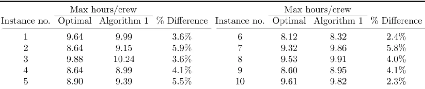
We implemented the LP-based algorithm to solve 100 randomly generated problem instances. In each problem instance, there are 70 jobs to be scheduled (with durations randomly drawn between 0 to 8 hours), 7 days in the planning horizon, and 3 crews available each day. For simplicity, we assume all jobs are due on the last day. Table 1 shows results for ten of the 100 problem instances.
Table 1 Maximum ratio of scheduled hours to number of crews under the optimal schedule and the schedule from Algorithm 1.
Max hours/crew Max hours/crew
Instance no. Optimal Algorithm 1 % Difference Instance no. Optimal Algorithm 1 % Difference
1 9.64 9.99 3.6% 6 8.12 8.32 2.4%
2 8.64 9.15 5.9% 7 9.32 9.86 5.8%
3 9.88 10.24 3.6% 8 9.53 9.91 4.0%
4 8.64 8.99 4.1% 9 8.60 8.95 4.1%
5 8.90 9.39 5.5% 10 9.61 9.82 2.3%
On average (over all 100 instances), the schedule from Algorithm 1 achieves a maximum ratio of scheduled hours to number of crews that is 5.3% greater than the optimal maximum ratio. However, Algorithm 1 manages to drastically improve computational efficiency. Solving for the optimal schedule in (4) sometimes requires several hours. On the other hand, Algorithm 1 only takes a few seconds to solve.
4.
Phase II: Crew Assignment
Let{x∗it} be the optimal solution to the scheduling phase problem. Fixing this job schedule
decom-poses the assignment phase to separate and independent crew assignment problems per day. We denote by It the set of job indices that are scheduled for day t. That is, It, {i : x∗it= 1}. For
each day t, the assignment phase assigns all standard jobs in Itto available crews. However, these
standard job assignments must be made before the number of leaks in day t is realized. Once the number of leaks is known, all gas leak jobs must be assigned to the available crews. The objective for each day t is to make the standard job assignments so that the expected maximum hours on day t is minimized.
For each day t, the assignment phase solves a two-stage mixed integer program. The first stage problem is: minimize Y Et[Ct(Y, L(ω))] subject to ∑ k∈Kt Yik= 1, i∈ It, Yik∈ {0, 1}, i∈ It, k∈ Kt, (9)
where Ct(Y, L(ω)) is defined similarly as in the full optimization model:
Ct(Y, L(ω)) , minimize Z maxk∈Kt { dLZk+ ∑ i∈It diYik } subject to ∑ k∈Kt Zk= L(ω) Zk∈Z + , k∈ Kt. (10)
Note that the term in the brackets of the objective function is the number of hours assigned to crew k during scenario ω and under the standard job assignments are given by Y .
As the following proposition shows, the assignment phase problem can also be rewritten as a mixed integer program. The proof is similar to that of Proposition 1 and is left to the appendix.
Proposition 3. The deterministic equivalent of the day t two-stage assignment phase
prob-lem (9) is the following mixed integer program. minimize V,Y,Z ∑ ω∈Ωt Pt(ω)V (ω) subject to dLZk(ω) + ∑ i∈It diYik≤ V (ω), ω∈ Ωt, k∈ Kt, ∑ k∈Kt Yik= 1, i∈ It, ∑ k∈Kt Zk(ω) = L(ω), ω∈ Ωt, Yik∈ {0, 1}, i∈ It, k∈ Kt Zk(ω)∈Z + , ω∈ Ωt, k∈ Kt. (11)
Two-stage stochastic programs are difficult to solve since the number of scenarios blow up the dimension of the resulting deterministic equivalent problem. There have been many solution meth-ods developed in the literature to solve general two-stage stochastic programs, usually by approx-imating the second-stage expected value function. For instance, a common method is based on Benders’ decomposition embedded in a branch and cut procedure (Laporte and Louveaux 1993). Others are Lamiri et al. (2008) who propose a local search method, and Godfrey and Powell (2002) who suggest nonlinear functional approximations of the second-stage value function based on sam-ple gradient information. However, these solution methods are difficult to imsam-plement. Moreover, since they are developed to solve general two-stage stochastic problems, they do not give insight on the optimal allocation of resources in anticipation of an uncertain number of urgent jobs. Later in Section 4.3, we exploit the particular problem structure of the assignment phase problem to propose an algorithm for assigning the standard jobs under a stochastic number of gas leak jobs (Algorithm 2). This heuristic is simple and is motivated by the structure of the optimal solution.
4.1. Stochastic model compared to using averages
The stochasticity of the number of gas leaks increases the computational complexity of the problem. However, we will now demonstrate why solving the two-stage stochastic optimization model (9) results in more robust assignments than a simple heuristic that ignores stochasticity. In particular,
Table 2 Maximum hours (over crews) of optimal assignment and assignment based on average number of leaks.
Scenario Probability OPT max hours AVG max hours
0 leaks 0.4 11.76 10.66
1 leak 0.2 11.77 10.66
2 leaks 0.4 11.83 18.28
Expected maximum hours 11.79 13.70 Note: OPT is the optimal solution to (9). AVG is the solution to (12) which optimizes against the average number of leaks
consider a heuristic which makes crew assignment decisions against the average expected number
of leaks. This heuristic solves:
minimize Y Ct(Y, Et[L(ω)]) subject to ∑ k∈Kt Yik= 1, i∈ It, Yik∈ {0, 1}, i∈ It, k∈ Kt, (12)
where Ct is defined in (10). We will refer to this heuristic as AVG, while the optimal assignment
solved in (9) will be referred to as OPT.
In the following simple example, we compare the maximum hours for each gas leak scenario under crew assignments from the AVG heuristic and the OPT heuristic. Suppose that there are 7 crews available, and 15 standard jobs need to be assigned. The job durations are between 1 hour and 7 hours (see Table 3). The gas leak job duration is 8 hours. The probability of 0 leaks is 40%, the probability of 1 leak is 20%, and the probability of 2 leaks is 40%. Note that the average number of gas leaks is 1. We are interested in comparing the two heuristics with respect to the maximum work hours under the different leak scenarios.
Table 2 summarizes the results. Under the OPT assignment, all the crews work less than 11.83 hours even if there are 2 gas leaks. Under the AVG assignment, all crews work less than 10.66 hours if there are between 0 to 1 gas leaks. However, if there are 2 gas leaks, then the AVG assignment results in at least one crew working 18.28 hours. That is, there is a 40% probability that a crew under the AVG assignment will be working 18.28 hours. Since OPT results in a crew assignment where all crews work less than 11.83 hours on any leak scenario, it is more robust to stochasticity of gas leaks. These results agree with Birge (1997) who demonstrated that in many real-world applications stochastic optimization models are superior to their deterministic counterparts.
4.2. Structure of the optimal crew assignment
In this subsection, we conduct computational experiments on several examples in order to gain insight into the structure of the optimal crew assignment solution to (9). We find that the optimal crew assignment satisfies some structural properties, which we will exploit in order to propose a simple crew assignment heuristic.
Table 3 Durations of standard jobs.
Job no. Duration Job no. Duration Job no. Duration
1 6.58 6 5.36 11 3.48
2 6.41 7 4.96 12 2.66
3 5.63 8 4.85 13 2.61
4 5.49 9 4.25 14 2.26
5 5.47 10 3.83 15 1.51
Table 4 Probability distributions of number of gas leaks.
Leak scenario
0 leaks 1 leak 2 leaks 3 leaks E[no. leaks] Stdev[no. leaks] Leak distribution 1 0.0 1.0 0.0 0.0 1.0 0.00 Leak distribution 2 0.1 0.8 0.1 0.0 1.0 0.45 Leak distribution 3 0.2 0.6 0.2 0.0 1.0 0.63 Leak distribution 4 0.4 0.2 0.4 0.0 1.0 0.89 Leak distribution 5 0.3 0.5 0.1 0.1 1.0 0.89 Leak distribution 6 0.4 0.3 0.2 0.1 1.0 1.00 Leak distribution 7 0.5 0.2 0.1 0.2 1.0 1.18
Suppose for a given day, there are a total of 7 crews available. There are 15 standard jobs that need to be assigned to these crews, with durations given by Table 3. There is an average of one gas leak per day, where each gas leak job takes 8 hours. However, in our experiments, we will vary the probability distribution of the random number of gas leaks. In particular, we have seven computational experiments, each experiment using a different gas leak distribution in Table 4.
The optimal solutions to the seven numerical examples are given in the appendix (Tables 13–19). The highlighted cells in each table means that the corresponding crew (column) is assigned to work on a gas leak job during the corresponding leak scenario (row). Based on these results, an observation we can make is that in the optimal solution, if a crew is assigned to work on a gas leak in a given leak scenario, that crew should also be assigned to work on a gas leak in a scenario where there are more gas leaks. This is formalized in the following proposition. The proof is in the appendix.
Proposition 4. There exists an optimal solution (Y∗, Z∗(ω), ω∈ Ω) to the stochastic
assign-ment problem (9) with the property that if L(ω1) < L(ω2) for some ω1, ω2∈ Ω, then for all k ∈ K,
Zk∗(ω1)≤ Zk∗(ω2).
Another property of the optimal assignment we observe is that the jobs that have short durations are often assigned to the crews that handle gas leak jobs. Jobs with the longest durations are assigned to crews that work exclusively on standard jobs. That is, in anticipation of a random
number of urgent jobs, it is optimal to keep some crews idle or only assign them short duration jobs. Based on this observation, and the monotonicity property of Proposition 4, we propose a
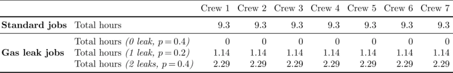
Table 5 Solution of LP relaxation of (11) with leak distribution 4.
Crew 1 Crew 2 Crew 3 Crew 4 Crew 5 Crew 6 Crew 7
Standard jobs Total hours 9.3 9.3 9.3 9.3 9.3 9.3 9.3
Gas leak jobs
Total hours (0 leak, p = 0.4) 0 0 0 0 0 0 0
Total hours (1 leak, p = 0.2) 1.14 1.14 1.14 1.14 1.14 1.14 1.14 Total hours (2 leaks, p = 0.4) 2.29 2.29 2.29 2.29 2.29 2.29 2.29
4.3. Assignment heuristic
Before introducing the assignment phase heuristic, recall that for the scheduling phase, we proposed a heuristic (Algorithm 1) based on solving the linear programming relaxation of the scheduling problem (6). The advantage of this heuristic compared to other sorting-based heuristics such as LG-LPT, is that it is easy to implement in optimization solvers such as Gurobi and CPLEX. In contrast, we now demonstrate through an example why it is inappropriate to solve the LP relaxation
of the assignment problem, when there is a stochastic number of emergencies arriving in the future.
Suppose that the LP relaxation of the assignment problem (11) is solved for one of the examples in the previous subsection (for leak distribution 4). The LP relaxation assumes that all jobs can be arbitrarily subdivided among several crews. Table 5 summarizes the optimal solution of the LP relaxation. From the table, the optimal LP solution evenly divides the gas leak hours among all the available crews in all leak scenarios. Hence, when there is one gas leak, all crews are assigned 1.14 gas leak hours. When there are two gas leaks, all crews are assigned 2.29 gas leak hours. The stochasticity of the number of gas leaks does not have any adverse effects on the first stage problem, since any gas leak hours can be borne by all crews. Hence, the optimal LP solution then ignores the effects of the second stage uncertainty and assigns the standard jobs to crews as evenly as possible. As discussed in Section 4.2, this solution is suboptimal since, if the jobs can’t be subdivided, the optimal crew assignment is to keep some crews dedicated to gas leak emergencies (compare with optimal crew assignment in Table 16 in the appendix).
Let us now describe the proposed assignment heuristic. This heuristic is a modification of the Longest-Processing-Time First (LPT) algorithm, to account for the presence of an uncertain num-ber of gas leak jobs. Recall that LPT is applicable when there is no uncertainty in the numnum-ber of gas leak jobs, and it assigns standard jobs to crews by first sorting the jobs by decreasing duration, and then one-by-one assigning the job to the crew with the smallest current load. In the proposed algorithm, gas leak jobs are first assigned for each leak scenario. Then, the algorithm sorts the standard jobs in decreasing order of duration. However, unlike LPT, the next job in the list is not assigned to the crew with the smallest current load (or expected load). Instead, it determines the increase in expected maximum hours by assigning to each crew. The job is assigned to the crew where this increase is the smallest. If there are any ties, the job is assigned to the crew with the
smallest expected current load. The outline of the algorithm is given in Algorithm 2. Note that when the number of gas leak jobs is deterministic, then this procedure is equivalent to LPT.
In the algorithm, the procedure for assigning the gas leak jobs for each scenario preserves the monotonicity property described in Proposition 4. It first sorts the gas leak scenarios in decreasing number of gas leaks. Starting with the first scenario, assign the gas leak jobs to crews using LPT. Now for the following scenarios, the gas leak jobs are also assigned to crews by LPT. However, in case of ties (where more than one crew has the minimum current load), choose a crew whose current load is strictly smaller than the load in the preceding scenario. This is done until all leak jobs for all scenarios have been assigned.
Algorithm 2 Assign to crews each standard job and gas leak job (for all leak scenarios).
Require: Ω ={ω1, ω2, . . . , ωm}, where L(ω1) < L(ω2) <· · · < L(ωm), and standard jobs sorted in
decreasing job duration, i.e. d1≥ d2≥ · · · ≥ dn
Ensure: Assignment of all standard jobs and gas leak jobs to crews under all leak scenarios
1: Bk(ωm+1)← 1, for all k ∈ K
2: for s = m to 1 do
3: Bk(ωs)← 0, for all k ∈ K
4: for l = 1 to L(ω2) do
5: K˜ ← arg mink∈K(Bk(ωs)){set of crews with smallest current load}
6: Bk0(ωs)← Bk0(ωs) + dL, where k0∈ ˜K such that Bk0(ωs) < Bk0(ωs+1)
7: end for 8: end for
9: for i = 1 to n do
10: for k∈ K do
11: B˜k(ω)← Bk(ω) + di, for all ω∈ Ω {Load in scenario ω if job i is assigned to crew k}
12: Ak(ω)← max
(
B1(ω), . . . , Bk−1(ω), ˜Bk(ω), Bk+1(ω), . . . , BK(ω)
)
, for all ω∈ Ω {Makespan in scenario ω if job i is assigned to crew k}
13: end for 14: Ki← arg mink∈K{ ∑ sP (ωs)Ak(ωs)} 15: k0∈ arg mink∈Ki{ ∑ sP (ωs)Bk(ωs)} 16: Bk0(ω)← ˜Bk0(ω), for all ω∈ Ω 17: end for
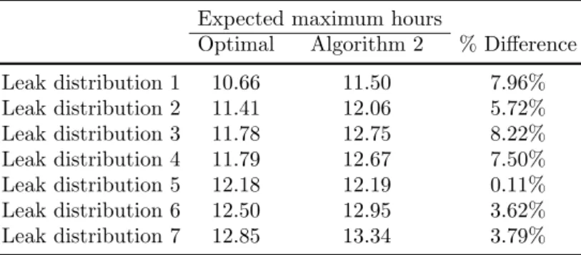
Using Algorithm 2, we assign jobs to crews for the seven numerical examples described in the pre-vious section. Table 6 compares expected maximum hours worked for the optimal crew assignment
Table 6 Expected maximum hours worked under the optimal crew assignment and the assignment from Algorithm 2.
Expected maximum hours
Optimal Algorithm 2 % Difference Leak distribution 1 10.66 11.50 7.96% Leak distribution 2 11.41 12.06 5.72% Leak distribution 3 11.78 12.75 8.22% Leak distribution 4 11.79 12.67 7.50% Leak distribution 5 12.18 12.19 0.11% Leak distribution 6 12.50 12.95 3.62% Leak distribution 7 12.85 13.34 3.79%
and the crew assignment resulting from Algorithm 2. Note that in the deterministic setting (Leak distribution 1), Algorithm 2 is equivalent to the LPT algorithm. Therefore, the worst-case bound of 56 for the difference applies, although the actual difference is much smaller (7.96%). Moreover, under all different gas leak distributions, Algorithm 2 results in expected maximum hours no more than 8.25% of the optimal. Recall that Table 4 summarizes the mean and standard deviation of number of leaks for the 7 distributions. Based on Table 6, it appears that Algorithm 2 results in a crew assignment that is closer to optimal when the distribution of gas leaks has a higher variance.
5.
Business analytics for the Gas business of a large multi-state utility
In this section, we describe how the research above applies to the scheduling of operations at the Gas business of a large multi-state utility. This is based on a joint project between the research team and the company that gave rise to the results of this paper. One of the company’s primary operations is the maintenance of a large network of gas pipeline. It keeps a roster of service crews who have two types of tasks: to execute standard jobs by their deadlines, and to immediately respond to gas leak emergencies. We discuss how we used the optimization models and heuristics described in this paper so that the company could develop better strategies to create flexibility in its resources to handle emergencies. We will show that the use of the model coupled with key process changes could help the company achieve significantly reduced costs and better ability to meet deadlines.
5.1. Overview of operations
The two types of jobs executed by crews have a few distinguishing features. Standard jobs have deadlines by when they must be finished, they are known several weeks to a few months in advance of their deadlines, and they are often mandated by regulatory authorities. These jobs include new gas pipeline construction, gas pipeline maintenance, replacement of gas pipelines, and customer requests. Emergency gas leak jobs are unpredictable, they need to be attended to immediately, they require several hours to complete, and they happen throughout a day. Currently, the company
maintains a centralized database of standard jobs which lists each job’s deadline, status (e.g. completed, pending or in progress), location, job type, other key job characteristics, and also information on all past jobs completed. The company also has a centralized emergency hotline that any member of the public can call in case of a suspected gas leak. In compliance with government regulations, the company’s policy is to respond to such reports within one or two hours of receiving them.
Both types of jobs for a particular geographical region (e.g., a town or several neighboring towns) are assigned to a nearby company site called a “yard”. Separate yards belonging to the company operate independently. Each yard houses a number of service crews who are responsible for executing both the standard jobs and the gas leak jobs for a geographical region. Small yards can have ten crews, while large yards can have up to 30 crews. Service crews have eight hour shifts, but can work beyond that if a job is taking too long or if there are many gas leak reports on that day. Any hours worked in excess of the crew’s shift is billed as overtime, and costs between 1.5 to 2 times the regular hourly wage. Aside from the service crews, each yard has crew supervisors. Each crew supervisor oversees several crews, typically 5 to 10. In addition, each yard has an employee called a resource planner who is charged with making decisions about the yard’s daily operations. In particular, at the start of each day, the resource planner looks over the pending jobs and decides on which jobs should be done by the yard, and which crews should execute these jobs.
5.2. Process mapping and data gathering
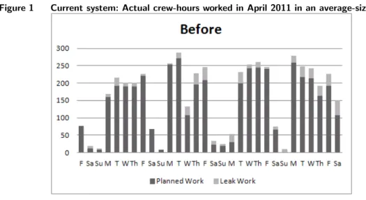
In order to understand sources of inefficiency of yard operations, we first set out to map in detail the existing yard processes. To do this, we gathered data about the yard operations in multiple ways. We visited several company yards and interviewed a number of resource planners, supervisors and crew leaders, as well as members of the Resource Management department (whose function is to set yearly and monthly targets for work to be performed in the field and to monitor the progress relative to these targets). We also did extensive job shadowing of crews from multiple yards performing different types of jobs, and documented the range of processes followed. Additionally, we also constructed historical job schedules based on data gathered from the company’s job database. Based on the gathered data, we found that crews in each yard have been working a significant proportion of their hours at overtime. In particular, an average crew member works 25% to 40% of his or her hours on overtime. Figure 1 shows the actual crew-hours worked in April 2011 for one of the company’s average-sized yards (with 25 weekday crews and 4 weekend crews). From Figure 1, we observe that even without the randomness introduced by the emergency gas leaks, the hours spent on working on standard jobs are unevenly divided among the workdays. We observed that one of the major causes of overtime is suboptimal job scheduling and planning for the occurrence of
Figure 1 Current system: Actual crew-hours worked in April 2011 in an average-sized yard.
gas leaks. Currently, the company has no guidelines or analytical tools for job scheduling and crew assignment. Instead, resource planners depend on their experience and feedback from supervisors. We also observed that availability of standard jobs fluctuates widely based on upstream processes of work order generation and permitting. Also, resource planners do not provide slack capacity (i.e., idle crew hours) to attend to any gas leak jobs that might occur later in the day. The combination of the uneven flow of standard jobs and the variability of emergency leaks put resource planners in a reactive mode resulting in a short planning horizon and suboptimal resource utilization. In addition, the company does not currently measure and analyze crew productivity. This results in resource planners relying on subjective input from supervisors on crew assignment decisions. Further, increasing the proportion of administrative work in the supervisors time has reduced time available for monitoring crew performance in the field. Past studies conducted by the company indicated the actual amount of time spent by supervisors in the field has significant impact on crew productivity, and hence, overtime.
5.3. Improving operations
Our project with the utility company had three main objectives. The first was to develop a tool that can be used with ease in the company’s daily resource allocation. Based on the models and heuristics we described in this paper, we created a tool – the Resource Allocation and Planning Tool (RAPT) – to optimally schedule jobs and to assign them to crews while providing flexibility for sudden arrival of gas leak emergencies. One of the major components of RAPT is the job scheduling and crew assignment models that we have described in the previous sections. For the tool to be practical, we ensured that it: (i) be simple to use, (ii) be straightforward to maintain, (iii) use popular software solutions, (iv) interface with the company’s multiple databases, and (v) be modular such that any changes can be made without too much difficulty. The tool uses a web-based
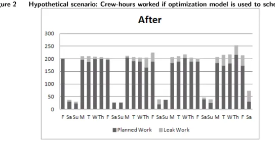
Figure 2 Hypothetical scenario: Crew-hours worked if optimization model is used to schedule jobs.
graphical user interface that is easy to use by resource planners. The back-end code was created based on Python and runs on a Windows-Apache-Oracle-Python stack on the company’s servers. It accesses the jobs database and the time-sheet database, and uses this historical information to estimate leak distributions and service times. These estimates and the list of all pending jobs are fed into the optimization models which are solved using Gurobi. RAPT outputs onto a webpage the weekly schedule for each crew and detailed plans under different gas leak scenarios.
The second objective was to create and improve processes related to daily resource allocation so that the tool could be easily embedded into daily scheduling process. We observed that a lot of the data in the database was either missing, inappropriately gathered or not vetted before entry into the system. Having missing or inaccurate data makes it very difficult to apply a data-driven tool such as RAPT and makes it even more difficult to address the right issues. Processes were created to ensure that when new jobs were added to the database, they had the right database fields set in a consistent manner across all jobs and yards. Prior to the project, certain job types were not entered into the database and were instead tracked on paper at each yard. The new processes fix these issues and add this information to the database. Resource planners, supervisors and crew members will be trained to familiarize them with the new process flows prior to implementation.
The third objective was to analyze the impact of key process and management drivers (business analytics) on operating costs and the ability to meet deadlines using the optimization model we developed. Results from this analysis will help the company deploy the optimization model with all the necessary process and management changes in order to capture the potential benefits outlined in this paper. The key process and management drivers selected for the study are work queues of available jobs for scheduling, availability of detailed productivity data (down to crew level) and supervisor presence in the field.
5.4. Business Analytics
Recall Figure 1 which shows the actual one-month profile of work hours in an average-sized yard. Figure 2 shows the profile for the same set of jobs if RAPT is used to assign and schedule those jobs. The result is a 65% decrease in overtime crew-hours for the month. However, this decrease in overtime assumes “perfect” conditions for the model—for example, that all the jobs are ready to be worked on at any date. Therefore, the 65% reduction in overtime hours is the maximum potential benefit of RAPT.
In reality, reaping the benefit of the model depends on the business processes currently estab-lished in the utility. Therefore, this reduction is most likely not achieved without first changing the company’s current processes. Using our models from this paper, we conducted a study to understand the impact of establishing new processes on yard productivity. Based on past stud-ies the company had conducted, the company understands that yard productivity is a complex phenomenon driven by process settings such as the size of work queues (i.e., jobs available for scheduling), effective supervision, incentives, and cultural factors. The research team and the com-pany agreed to analyze three specific drivers of productivity using RAPT: work queue level, use of crew-specific productivity data, and the degree of field supervision.
5.4.1. Optimal Work Queue Level. In reality, jobs need to be in a “workable” state before
crews can actually perform them. For example, the company needs to apply for a permit with the city before actually working on the job. Jobs in a “workable jobs queue” are jobs ready to be scheduled by RAPT. The reason why a queue is maintained is because “workable” jobs are subject to expiration and require maintenance to remain in a workable state (e.g., permits need to be kept up-to-date). The larger the job queue, the larger the opportunity of the tool to optimize job scheduling and crew assignment over the planning horizon. During the project, we observed some yards kept a low level of jobs in the workable jobs queue. The low workable jobs queue adversely impacted the RAPT output by not fully utilizing the tool’s potential. The team decided to run simulations to determine the strategic target level for the workable jobs queue to maximize the impact of RAPT while minimizing the efforts to sustain the workable jobs queue level.
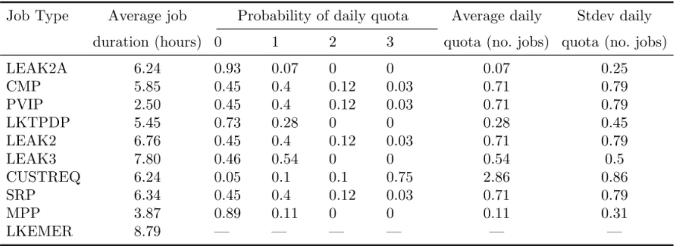
For our simulations we used actual data based on one of the company’s yard. Each day, there are five crews available in the simulated yard each with 8 hour shifts. There are ten different job types to be done (refer to Table 7). The job type LKEMER refers to emergency gas leaks that are stochastic in our model. The table also gives the average job duration for each job type. On each day, the Resource Management department announces a minimum quota of the number of jobs required to be done for each type. These quotas are random and depend on various factors beyond the yard’s control. Based on historical quotas, we estimate the probability distribution of
daily quotas for each job type (Table 7). To be able to meet the daily quota requirements, the yard maintains a workable jobs queue for each job type. As an example, suppose that today the quota for CMP jobs is 10. However, there are only 6 jobs in the workable CMP job queue. Then, today, the yard will work on 6 CMP jobs, and will carry over the remaining 4 CMP jobs as a backlog for the next day. Each time the yard requests for new workable jobs to be added to the queue, there is a lead time of 3 days before the request arrives. For instance, this lead time may include time used for administrative work to apply for a permit.
Table 7 Data for job types used for simulations.
Job Type Average job Probability of daily quota Average daily Stdev daily duration (hours) 0 1 2 3 quota (no. jobs) quota (no. jobs)
LEAK2A 6.24 0.93 0.07 0 0 0.07 0.25 CMP 5.85 0.45 0.4 0.12 0.03 0.71 0.79 PVIP 2.50 0.45 0.4 0.12 0.03 0.71 0.79 LKTPDP 5.45 0.73 0.28 0 0 0.28 0.45 LEAK2 6.76 0.45 0.4 0.12 0.03 0.71 0.79 LEAK3 7.80 0.46 0.54 0 0 0.54 0.5 CUSTREQ 6.24 0.05 0.1 0.1 0.75 2.86 0.86 SRP 6.34 0.45 0.4 0.12 0.03 0.71 0.79 MPP 3.87 0.89 0.11 0 0 0.11 0.31 LKEMER 8.79 — — — — — —
The yard adapts a continuous review policy for the workable jobs queue specified by a reorder
point and an order quantity. Each time the total workable jobs (both in the queue and in the
pipeline) drops below the reorder point, the yard requests new workable jobs. The size of the request is equal to the order quantity. The request is added to the pipeline and arrives after a lead time of 3 days. As an example, suppose the yard chooses a reorder point of 2 and an order quantity of 10 for the CMP workable jobs queue. Then, each time the total CMP workable jobs drops below 2, then the yard places an additional request for 10 workable CMP jobs. In our simulations, the order quantity is set for each job type queue so that, on average, new requests are made every week. The reorder point is determined from a service level the yard chooses, where the service level is the probability that there is enough jobs in the workable jobs queue to meet new quotas during the lead time period (i.e., while waiting for new workable jobs to arrive). For each simulated day, quotas are generated based on Table 7 and met to the maximum extent possible from the workable jobs queue. The jobs are assigned to the 5 crews using the RAPT crew assignment model. In our simulations, we will determine the effect of the service level α on: (i) the average number of workable jobs kept in the queues, (ii) the number of backlogged quotas, and (iii) the day-to-day crew utilization.
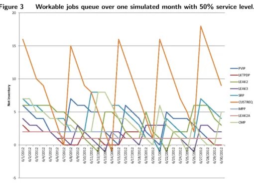
Figure 3 Workable jobs queue over one simulated month with 50% service level.
Figure 3 shows the evolution of the workable jobs queue in one simulated month for a 50% service level. The net inventory level corresponds to the total number of workable jobs currently in the queue. When the net inventory is negative, then there is a backlog of workable jobs for that job type (i.e., there are not enough workable jobs to meet the quotas). Table 8 summarizes the results of the simulation for different service levels. Note that increasing the service level increases the average size of the workable jobs queues, resulting in a smaller probability of backlogged jobs. With 50% service level, the average inventory per day in the workable jobs queue is 28.8. However, a total of 7 quotas have not been met in time. Increasing the service level to 75% requires increasing the average inventory per day to 35.6, resulting in eliminating any backlogged jobs. Increasing the service level further to 90% or 99% results in higher average inventories of workable jobs, but with essentially the same effect on backlogged jobs as the smaller service level 75%.
Table 8 Effect of service levels on average workable jobs inventory, backlogged jobs, and overtime crew-hours for one simulated month.
Service Level 50% 75% 90% 99%
Average inventory per day 28.8 35.6 37.6 50.6
Total backlogged jobs 7 0 0 0
Average overtime per day (crew-hours) 14.67 14.55 14.55 14.55 Standard deviation overtime per day (crew-hours) 8.92 8.26 8.26 8.26
In fact, having a backlog of quotas also has an effect on the day-to-day crew utilization. For example, in Figure 3 lack of CUSTREQ workable jobs on June 14 meant that crews were
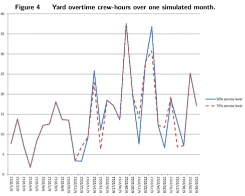
under-Figure 4 Yard overtime crew-hours over one simulated month.
utilized on that day. However, after workable jobs arrive on June 15, not only do crews have to work on quotas meant for June 15, they also need to be working on the jobs to meet the missed quotas for June 14. In the perfect setting of an infinite supply of workable jobs, crews will be working on average the same amount of hours. Having finite supply of workable jobs means that crew utilization is variable from day-to-day. Figure 4 shows the total expected overtime in one simulated month. Notice that for a 50% service level, the “peaks” and “valleys” of overtime hours are more pronounced. It is important to note that this fluctuation is artificial since it is caused by the inventory policy for the workable jobs queue. This is obvious when comparing it to the overtime hours with a 75% service level, where crews are utilized at a more even rate. The plots for overtime hours under a 90% and 99% service level is the same as under a 75% service since they all result in no backlogged jobs.
5.4.2. Appropriateness of Productivity Data. Presently detailed crew productivity is not
available. As such, it is not possible to make crew assignments to take advantage of the inherent job-specific productivity differences between crews in the crew assignment phase. In consultation with company management, we decided to study the impact of capturing and using job-specific productivity data in crew assignment versus assigning jobs based on average productivity.
Table 9 Job type and crew expertise.
CREW1 CREW2 CREW3 CREW4 CREW5 Expertise LKEMER CMP PVIP LEAK2 SRP