HAL Id: hal-01511667
https://hal.archives-ouvertes.fr/hal-01511667
Preprint submitted on 21 Apr 2017HAL is a multi-disciplinary open access archive for the deposit and dissemination of sci-entific research documents, whether they are pub-lished or not. The documents may come from teaching and research institutions in France or abroad, or from public or private research centers.
L’archive ouverte pluridisciplinaire HAL, est destinée au dépôt et à la diffusion de documents scientifiques de niveau recherche, publiés ou non, émanant des établissements d’enseignement et de recherche français ou étrangers, des laboratoires publics ou privés.
The stability of short-term interest rates pass-through in
the euro area during the financial market and sovereign
debt crises
Sanvi Avouyi-Dovi, Guillaume Horny, Patrick Sevestre
To cite this version:
Sanvi Avouyi-Dovi, Guillaume Horny, Patrick Sevestre. The stability of short-term interest rates pass-through in the euro area during the financial market and sovereign debt crises. 2017. �hal-01511667�
DOCUMENT
DE TRAVAIL
N° 547
THE STABILITY OF SHORT-TERM INTEREST RATES PASS-THROUGH IN THE EURO AREA DURING
THE FINANCIAL MARKET AND SOVEREIGN DEBT CRISES
Sanvi Avouyi-Dovi, Guillaume Horny and Patrick Sevestre April 2015
DIRECTION GÉNÉRALE DES ÉTUDES ET DES RELATIONS INTERNATIONALES
THE STABILITY OF SHORT-TERM INTEREST RATES PASS-THROUGH IN THE EURO AREA DURING
THE FINANCIAL MARKET AND SOVEREIGN DEBT CRISES
Sanvi Avouyi-Dovi, Guillaume Horny and Patrick Sevestre April 2015
Les Documents de travail reflètent les idées personnelles de leurs auteurs et n'expriment pas nécessairement la position de la Banque de France. Ce document est disponible sur le site internet de la Banque de France « www.banque-france.fr ».
Working Papers reflect the opinions of the authors and do not necessarily express the views of the Banque de France. This document is available on the Banque de France Website “www.banque-france.fr”.
The stability of short-term interest rates pass-through in the euro area
during the financial market and sovereign debt crises
S. Avouyi-Dovi*, G. Horny** and P. Sevestre***
* Banque de France, 31 rue Croix des Petits Champs, 75001, Paris, France and Leda-SDFi, Université Paris-Dauphine. E-mail: Sanvi.Avouyi-Dovi@banque-france.fr
** Banque de France, 31 rue Croix des Petits Champs, 75001, Paris, France. E-mail:
Guillaume.Horny@banque-france.fr
*** Aix-Marseille University (Aix-Marseille School of Economics). E-mail: patrick.Sevestre@univ-amu.fr We would like to thank an anonymous associate editor, two anonymous referees, Robert Bliss, Nicola Borri, Selva Demiralp and Ipek Mumcu for their detailed and helpful suggestions. We would also like to thank participants in the ERUDITE seminar and to the INFINITI 2014 conference for their comments. Part of the work was carried out while Patrick Sevestre was at the Banque de France. The views expressed in this article are those of the authors and do not necessarily reflect the views of the Banque de France, Université Paris-Dauphine or Aix-Marseille School of Economics.
Résumé
Nous étudions la dynamique de la transmission du coût marginal des banques aux taux à court terme des nouveaux crédits bancaires accordés aux sociétés non financières, en Allemagne, Espagne, France, Grèce, Italie et Portugal, au cours de la crise financière de 2008 et de celle des dettes souveraines. Nous mesurons le coût marginal des banques par les taux des nouveaux dépôts alors que l'accent est mis sur les taux du marché monétaire dans la littérature. Cela nous permet de différencier le risque auquel font face les banques dans les différents pays. Nous spécifions un modèle à correction d'erreur que nous généralisons, d’une part, pour permettre à la relation de long terme liant le taux des crédits bancaires au coût marginal des banques de changer dans le temps, et, d’autre part, pour introduire une volatilité stochastique. Le modèle est estimé avec des données, harmonisées entre les pays étudiés, et couvrant la période allant de Janvier 2003 à Octobre 2014. Nous utilisons une approche bayésienne, basée sur des méthodes de Monte Carlo par Chaînes de Markov (MCCM). Nos résultats rejettent l'hypothèse selon laquelle le coût marginal des banques se transmet aux taux des nouveaux crédits de manière constante dans le temps. La relation de long terme qui unit ces variables, s’est modifiée avec la crise de la dette souveraine ; elle est devenue une relation dans laquelle les variations de coût marginal se transmettent plus lentement et où les taux des prêts bancaires sont plus élevés. Ces évolutions diffèrent d'un pays à l'autre. En effet, les freins à la transmission des taux monétaires dépendent de l'hétérogénéité des coûts marginaux des banques, et donc de leurs risques. Nous constatons également que dans certains pays, les taux accordés aux petites entreprises augmentent par rapport à ceux octroyés aux grandes entreprises durant la crise. Enfin, avec un modèle VAR, nous montrons que, globalement, un choc sur les taux des nouveaux dépôts à moins d’effet sur l’évolution des taux des nouveaux prêts depuis 2010. Ces résultats confirment le ralentissement dans la transmission.
Mots clés : taux bancaires, modèle à correction d’erreur, ruptures structurelles, volatilité stochastique, économétrie bayésienne.
Classification JEL: E430, G210.
Abstract
We analyse the dynamics of the pass-through of banks’ marginal cost to bank lending rates over the 2008 crisis and the euro area sovereign debt crisis in France, Germany, Greece, Italy, Portugal and Spain. We measure banks’ marginal cost by their rate on new deposits, contrary to the literature that focuses on money market rates. This allows us to account for banks’ risks. We focus on the interest rate on new short-term loans granted to non-financial corporations in these countries. Our analysis is based on an error-correction approach that we extend to handle the time-varying long-run relationship between banks’ lending rates and banks’ marginal cost, as well as stochastic volatility. Our empirical results are based on a harmonised monthly database from January 2003 to October 2014. We estimate the model within a Bayesian framework, using Markov Chain Monte Carlo methods (MCMC).We reject the view that the transmission mechanism is time invariant. The long-run relationship moved with the sovereign debt crises to a new one, with a slower pass-through and higher bank lending rates. Its developments are heterogeneous from one country to the other. Impediments to the transmission of monetary rates depend on the heterogeneity in banks marginal costs and therefore, its risks. We also find that rates to small firms increase compared to large firms in a few countries. Using a VAR model, we show that overall, the effect of a shock on the rate of new deposits on the unexpected variances of new loans has been less important since 2010. These results confirm the slowdown in the transmission mechanism.
Keywords: bank interest rates, error-correction model, structural breaks, stochastic volatility, Bayesian econometrics.
Non-technical summary
After the 2008 financial crisis and the ensuing Great Recession, major monetary authorities shifted to an accommodative policy stance. Interest rates on new bank loans decreased accordingly, but questions have been raised about the transmission of such an accommodative policy stance to the economy. Because funding in the Euro area is mostly bank based, a breakdown in the transmission to bank lending rates would be a major obstacle to the conduct of its monetary policy.
This paper explores the issue of heterogeneous development in the price of new bank loans in relation to structural changes in banks’ marginal cost. We hence pay particular attention to developments in the transmission mechanism over time. Therefore, we focus on a set of countries made of the so-called core countries (France and Germany), countries heavily hit by the sovereign debt crisis (Greece and Portugal), and countries in between (Italy and Spain). To further help in performing relevant comparisons, we draw data from the Monetary Interest Rate (MIR) survey database, which are harmonised at the level of the euro area countries and we consider the identical time span from January 2003 to October 2014.
We depart from the standard analyses of the transmission mechanism, with several contributions. First, we run statistical tests to identify change points in the transmission mechanism. This is important as shocks or major policy events can interrupt the co-movement of variables, possibly for an extended period of time. Second, we adapt our model to take into account changes in the co-movement among variables, something generally assumed constant in this literature. Third, this literature focuses on the transmission of policy rates to bank rates on new loans. We assess the importance of taking into account country risks in the cost of banks’ resources, which therefore depart from the policy rates. The literature generally investigates rates on loans with different maturities. For the sake of clarity and robustness, we focus on the price of short-term credit, meaning loans with a maturity up to one year. We relate it to the rate on new deposits with a maturity of less than one year. It reacts to features such as access to financial markets, country risks, banks’ and borrowers’ risks. The rate on new deposits is therefore close to the cost of wholesale funding paid by banks.
Our main results are summarized as follows: 1) we reject the view that the long-run relationship between the banks’ lending rates and the banks’ marginal costs remain unchanged over the last crises. Assuming this relationship is permanent, as commonly done in studies preceding the 2008 crisis, is now irrelevant. We also show that the most important changes have occurred since the onset of the sovereign debt crisis. Therefore, it is not the financial crisis that is directly at the origin of the slowdown in the pass-through. On the opposite, changes in banks’ marginal costs in the wake of the financial crisis have been transmitted to the rates on new loans especially quickly; 2) indications of an impairment of the transmission mechanism become less prevalent when we measure the cost of bank resources with rates on deposits rather than with rates set on the interbank market. The breakdown in the pass-through mechanism of the policy rates result from the lack of control for risk in the measure of banks’ cost; 3) simulated bank lending rates indicate that the new pass-through mechanism implies higher rates than the ones that would have been observed with the relationship prevailing before the 2008 crisis. After 2010, the decrease in the cost of bank resources was followed by a decrease in the rate on new bank loans of a far lesser magnitude than what we can expect against the background of the relationship prevailing before 2008; 4) whereas our results for the financial crisis are in line with some rationing scheme, those for the sovereign debt crisis indicate an increase in banks’ spreads, compatible with greater bank funding difficulties. The increase in banks’ mark-ups is especially pronounced on loans to smaller, thus more risky, borrowers. It seems therefore plausible that non-financial corporations’ default risk became suddenly more important, or more heavily priced, with the sovereign debt crisis; 5) developments in the pass-through mechanism are heterogeneous. Thus, impairment of the transmission of the accommodative monetary policy stance is more problematic for some countries than for others.
1. Introduction
After the 2008 financial crisis and the ensuing Great Recession, major monetary authorities shifted to an accommodative policy stance. They cut policy rates down to near-zero and simultaneously engaged in massive unconventional monetary policy programs. Interest rates on new bank loans decreased accordingly, but questions have been raised about the transmission of such an accommodative policy stance to the economy. The European Central Bank (ECB) often refers to the pass-through of its programs to the main economic variables and expressed concerns on impediments to the transmission mechanism (see for instance ECB (2013), (2014)). Because funding in the Euro area is mostly bank based, a breakdown in the transmission to bank lending rates would be a major obstacle to the conduct of its monetary policy. These concerns are supported by several recent studies pointing to a reduction of the degree of pass-through from the money market rate, including Aristei and Gallo (2014), Belke
et al. (2013), Hristov et al. (2014), and Ritz and Walther (2015) among others.
While recent literature highlights the deterioration in the pass-through since the financial crisis, it provides little guidance on what changes occur in the way banks set their interest rate. Implicitly, this literature considers banks’ own access to funding as constant in the long-run, meaning its variations during times of crises are not accounted for. This is questionable as the whole period experienced deep changes, including peaks in banks’ own credit risks and changes in their regulation.1
This paper explores the issue of heterogeneous development in the price of new bank loans in relation to structural changes in banks’ marginal cost. We hence pay particular attention to developments in the transmission mechanism over time. We depart from the standard analyses of the transmission mechanism, based either on Error-Correction models or Vector AutoRegressive (VAR) analysis, with three contributions. First, we use statistical tests to identify change points in the transmission mechanism. This is important as shocks or major policy events can interrupt cointegration relationships, possibly for an extended period of time (Siklos and Granger, (1997)). Second, whereas mean or variance parameters are generally assumed constant in this literature, we contribute to it by relaxing both assumptions simultaneously. Third, this literature focuses on the transmission of policy rates to bank rates on new loans. We assess the importance of taking into account country risks in the cost of banks’ resources, which therefore depart from the policy rates.
Our paper is directly connected to the interest rate channel of monetary policy. Mojon (2000), Toolsema et al. (2001), Angeloni et al. (2003), Sander and Kleimeier (2004), de Bondt (2005), Kleimeier and Sander (2006), Marotta (2009), among others, analyzed the transmission mechanism of the rates set by the monetary authorities to the rate on new loans in the euro area during the inception or the start of the Monetary Union. The main findings of these studies are the following: 1) the pass-through from the money market rates to bank lending rates is not complete, but rates on short-term loans react more fully and faster than those on longer maturities; 2) adjustments are quicker for corporate borrowers than for households; 3) there is a strong heterogeneity across countries in the pass-through mechanisms.
The literature generally investigates rates on loans with different maturities. For the sake of clarity and robustness, we focus on the price of short-term credit, meaning loans with a maturity up to one year. As a consequence, we restrict ourselves to credit markets where the pass-through is generally quick and close to complete. Our choice is motivated for three reasons. Firstly, since long-term rates are obtained by rolling over short-term rates, a weakening in the transmission mechanism at short horizons will manifest itself at long-horizons. Secondly, banks’ short-term rates do not come from intertemporal optimizations over long time horizons. Their dynamics do not involve expectations on distant risks, for instance general redenomination risk. Thirdly, banks transform securities with short
1 Changes in banks’ credit risk should impact their marginal cost, as lenders and depositors ask for a higher compensation to take the risk,
preventing some banks to access the financial market or attract enough deposits. Tighter macroprudential regulations provide incentives to banks to increase their mark-up. A thorough discussion of the underlying economic mechanism can be found in Darracq-Parriès et al. (2011).
maturities, offered to depositors, into securities with long maturities, demanded by borrowers. The maturity transformation makes debateable that there is a direct matching on the maturity between banks’ assets and liabilities. Focusing on short-term loans makes the construction of a measure of banks’ marginal cost especially robust to maturity mismatch issues.
In our application, we use as banks’ marginal cost the rate on new deposits with a maturity of less than one year. It reacts to features such as access to financial markets, country risks, banks’ and borrowers’ risks. The rate on new deposits is therefore close to the cost of wholesale funding paid by banks. Alternative measures include several rates on the interbank market. However, money market rates provide interest rates that do not reflect the heterogeneity among banks. Since the 2008 crisis, activity on the interbank market is limited and it is likely that the riskier banks cannot borrow from it. We provide also sensitivity analysis where the marginal cost is approximated by the overnight interest rate or the 3-month and 6-month Euribor.
The main question of our paper can be rephrased as to whether some countries disassociate from others. We therefore focus on a set of countries made of the so-called core countries (France and Germany), countries heavily hit by the sovereign debt crisis (Greece and Portugal), and countries in between (Italy and Spain). To further help in performing relevant comparisons, we draw data from the Monetary Interest Rate (MIR) survey database, which are harmonised at the level of the euro area and we consider the identical time span from January 2003 to October 2014.
We model bank short-term rate dynamics with an error-correction approach, in line with an abundant literature initiated by Cottarelli and Kourelis (1994) in which loan prices and banks’ marginal cost are related. This approach focuses on the pass-through of a change in costs to a change in price. The model is directly related to oligopolistic theories of competitions where banks are implicitly viewed as price makers.
We extend the basic model in order to take into account the peculiarity of the time period under review, characterized by the financial and the European sovereign debt crises. First, we test for the existence of breaks using multiple procedures and date them following Bai and Perron (1998) tests. Since the breakdates are returned along with confidence intervals, we set accurate breaks using additional economic and financial information. Second, we echo back Siklos and Granger’s (1997) concept of regime-sensitive cointegration. Intuitively, several relationships among variables are possible and one can deviate from a specific equilibrium after some major events. As a consequence, the series may be cointegrated over some periods but not in others, and the model must allow the pass-through mechanism to change over time periods. In other words, the parameters of the error-correction equation are assumed to vary over different time periods. Third, since we allow for drifting parameters in the mean, we also have to allow for time-varying variances. Indeed, if we fit the model assuming time-varying parameters in the mean and constant parameters in the variance while the true model is also based on the time-varying hypothesis of the variance parameters, how can we ensure that the mean parameters do not drift to compensate for misspecification? This is especially important over a time of high stress such as the one that occurred over the last few years. In time of crises, a model with constant parameters in the mean and time-varying variance would attribute the high observed variance to an increase in the innovation variances. While a model with time-varying parameters in the mean and constant variance would attribute it to a change in the transmission mechanism. These two reasons led us to impose, in our most general framework, the assumption of time-varying parameters in both the mean and the variance equations of the bank lending rate (McConnell and Perez-Quiroz (2000)).2
In other words, our model combines two types of shocks. First, it allows for departure from a given equilibrium due to major events. Second, it allows for deviations of potentially high magnitudes to occur without altering the equilibrium. We estimate the model using a Bayesian approach based on the Gibbs sampler. We also complement our main analysis with a VAR analysis.
2 Alternatively, we could have investigated models with the Markov switching as in McConnell and Perez-Quiroz (2000).
Our main results are summarized as follows: 1) we reject the view that the long-run relationship between the banks’ lending rates and the banks’ marginal costs remain unchanged over the last crises. Assuming this relationship is permanent, as commonly done in studies preceding the 2008 crisis, is now insufficient. We also show that the most important changes have occurred since the onset of the sovereign debt crisis. These results are confirmed by the VAR analysis. It is therefore not the financial crisis that is directly at the origin of the slowdown in the pass-through. On the opposite, changes in banks’ marginal costs in the wake of the financial crisis have been transmitted to the rates on new loans especially quickly; 2) indications of an impairment of the transmission mechanism become less prevalent when we measure the cost of bank resources with rates on deposits rather than with rates set on the interbank market. The breakdown in the pass-through mechanism of the policy rates result from the lack of control for risk in the measure of banks’ cost; 3) simulated bank lending rates indicate that the new pass-through mechanism implies higher rates than the ones that would have been observed with the relationship prevailing before the 2008 crisis. After 2010, the decrease in the cost of bank resources was followed by a decrease in the rate on new bank loans of a far lesser magnitude than what we can expect against the background of the relationship prevailing before 2008; 4) whereas our results for the financial crisis are in line with some rationing scheme, those for the sovereign debt crisis indicate an increase in banks’ spreads, compatible with greater bank funding difficulties. The increase in banks’ mark-ups is especially pronounced on loans to smaller, thus more risky, borrowers. It seems therefore plausible that non-financial corporations’ default risk became suddenly more important, or more heavily priced, with the sovereign debt crisis; 5) developments in the pass-through mechanism are heterogeneous. Thus, impairment of the transmission of the accommodative monetary policy stance is more problematic for some countries than for others.
Our approach is also related to two methodological literatures: the first on error-correction models and the second on stochastic volatility (SV) models of which the treatment in the Bayesian framework was introduced by Jacquier et al. (1994). Indeed, they provide a MCMC procedure, referred to as a single move procedure, where the latent log-volatilities are sampled one at a time. Kim et al. (1998) provide a procedure to jointly sample the log-volatilities, known as a multi-move MCMC algorithm. Jacquier
et al. (2010) apply the recent development on particle filters by Carvalho et al. (2010) to SV models.
Our study is connected to the literature on asymmetries in the pass-through. This body of the literature includes Hofmann and Mizen, (2004), Sander and Kleimeier (2004), Rocha (2012), Belke et al. (2013), Yüksel and Metin Ozcan (2013), among others. The main result is that the interest rate dynamics differ between times of easing and times of tightening in the monetary policy. More specific results seem to be quite sensitive to the country, the period and the type of loans studied. For instance, Becker et al. (2012) show that in a stable environment, decreases in the policy rates are not fully passed on. This echo back to results obtained more generally in the literature on price-setting: increases in costs are passed-through to prices more quickly than decreases.
Our paper is also linked to the literature on bank lending rates using micro-data. For instance, with data at the individual loan-level, Berger and Udell (1992) show that bank rates are stickier than Treasury bill rates. Hannan and Berger (1991) and van Leuvensteijn et al. (2013) conclude that the rigidity of bank rates depends on the competition among banks. Banerjee et al. (2013) explicitly introduce the banks’ expectations hypothesis in their lending rates dynamics. Many studies conclude that the pass-through depends on the characteristics of banks, leading to the analysis of the bank lending channel (Kashyap and Stein (2000), Kishan and Opiela (2000), Altunbas et al. (2002), Barbier de la Serre et al. (2008), Gambacorta (2008)).
The paper proceeds as follows. Section 2 is devoted to the data, the characteristics of banks lending rates as well as the choice of a variable to measure banks’ marginal cost. Section 3 presents the pass-through model and the Bayesian inference. Empirical results are reported in Section 4, as well as their implications for the volatility and the interest rate setting. Sensitivity analysis to alternative measures of banks marginal costs and VAR analysis are also conducted in this section. Section 5 concludes.
2.
Bank short rate data
An empirical analysis of the pass-through of the cost of bank resources via the credit channel requires a reliable measure of the interest rates applied by Monetary and Financial Institutions (MFIs). In order to make these interest rates comparable in the euro area, the ECB decided in December 2001 to standardise the existing surveys previously conducted by the national central banks. This led to the MFI Interest Rates (MIR) survey, in which the types of rates, financial instruments, reporting populations and methods of calculation are harmonised.3 The resulting data are aggregated over loan
contracts at the national level.
2.1. Data description
Interest rates are expressed as annual percentage rates at the aggregate levels, which are derived from new individual contracts agreed between a MFI and a non-financial corporation (NFC). New agreements are all financial contracts that specify the interest rates on the loans for the first time, and all renegotiations of existing loans. New business therefore does not include automatic extensions of existing contracts that do not involve any renegotiation of the terms and conditions. Revolving loans and overdrafts, as well as convenience and extended credit card debt, are also excluded from the underlying sample. Agreed rates can be lower than advertised rates because the customer is able to negotiate a better rate. The MFI interest rate statistics on new business hence reflect the agreed conditions on the loan market at the time of the contract. Therefore, they reflect demand and supply, including variations in the cost of funds faced by banks, competition between banks, and types of financial institutions and products.
As previously mentioned, the dataset has been drawn from the MIR survey. It consists of monthly observations on new loans with maturity up to one year to non-financial corporations. It spans from January 2003 to October 2014. We use data on the loans granted in France, Germany, Greece, Italy, Portugal and Spain.
2.2. Main features of the interest rates on new short-term loans
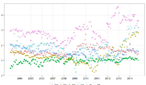
Figure 1 displays the evolution of bank interest rates on new loans with a maturity up to one year in the countries under review. Despite differences in their levels, interest rates appear to comove remarkably up to early 2010. While they remained fairly stable or even decreased slightly between 2003 and the end of 2005, they began to rise in 2006 until the third quarter of 2008. Following the failure of Lehman Brothers in September 2008, they fell at the end of 2009 in these six countries by about 325 basis points on average. Short rates split into three groups from the beginning of 2010: they varied but remained lower than their mean over the sub-period 2003-2006 in the first group (Germany and France); they rose again from 2010 up to levels close to those observed just before September 2008 and then decreased progressively in the second group (Greece and Portugal); the last group was composed of Italy and Spain, whose interest rates were in an intermediate situation. These three sub-groups of countries were more or less confirmed at the end of the period under review (October 2014).
Figure 1: Monetary and financial institutions’ interest rates to non-financial corporations Maturity up to one year, January 2003-October 2014
Source: MIR survey, ECB
The traditional stationary tests showed that interest rates are integrated of order 1 (I(1)). As a consequence, we focus then on their first-order difference (Figure A.1 in the Appendix). Three main remarks can be made. First, as mentioned above, the increase in short rates from 2006 to 2008 is gradual and made up of small variations. This translates into slightly positive values of the difference in interest rates between 2006 and 2008. Second, we observe a sharp decline in rates from September 2008 to December 2009, yielding huge negative variations in the series in difference for all countries. Third, changes in interest rates in Spain and Greece are greater after 2010 than before September 2008. Indeed, the increase of the interest rates is steeper between 2010 and 2012 than between 2006 and 2008. From 2013 to October 2014, the interest rates dramatically declined in the three sub-groups of the euro area countries. However, the decrease in the interest rates has been more marked for Italy and Spain since January 2014.
Table 1 reports descriptive statistics on changes in interest rates. The averages of the first-order differences of interest rates are close to zero, as they range from -2 basis points (Germany) to 1 basis point (Greece). The standard deviations range from 17 basis points (Germany) to 30 basis points (Greece). As the medians are positive, it is likely the means reflect the sharp negative variations that occurred between September 2008 and December 2009. This is reinforced by the negative skewness for all countries, meaning that the left tail of the probability density function is longer than the right one, and that interest rates mostly lie to the right of the mean. The largest drop in interest rates (-124 basis points) occurred in France from December 2008 to January 2009. The excess kurtosis for France is the highest (at about 14), indicating a density with a sharper peak and fatter tails than in the other countries, where the densities are already more peaked and with fatter tails than in the Gaussian case.
Table 1: Summary statistics and p-values of tests on changes in MFIs’ interest rates (in basis points, February 2003-October 2014) DE ES FR GR IT PT Descriptives statistics Mean -1.71 -0.44 -0.95 0.61 -1.04 -0.44 Median 0.00 2.00 1.00 2.00 1.00 1.50 Sd 16.85 19.72 19.61 30.49 17.13 23.29 Min -72.00 -78.00 -124.00 -98.00 -75.00 -86.00 Max 32.00 62.00 29.00 117.00 34.00 57.00 Skewness -1.30 -1.05 -2.80 -0.09 -1.28 -0.56 Excess Kurtosis 3.63 3.82 14.30 2.43 3.83 0.96 Stationarity tests Phillips-Perron 0.00 0.00 0.00 0.00 0.00 0.00 ADF 0.01 0.01 0.01 0.01 0.01 0.01 Heteroskedasticity and autocorrelation tests Ljung-Box 0.00 0.00 0.00 0.00 0.00 0.03 Diebold 0.03 0.01 0.02 0.05 0.03 0.03 ARCH-LM 0.00 0.00 0.00 0.00 0.00 0.03 Note: Ljung-Box, Diebold and ARCH p-values are computed using lags over three months.
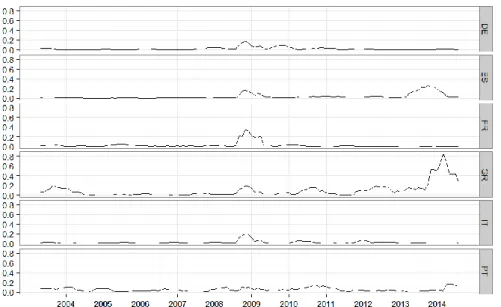
To check the intuition that time-varying variances characterise the interest rates dynamics, we calculate the rolling variances of the first-order differences of the interest rates. Figure 2 shows that the rolling variances peak at the end of 2008 and the beginning of 2009 for all countries but Portugal. In the case of Greece and Spain, this is followed by even larger peaks since early 2013. In addition, ARCH-LM tests allow us to reject the hypothesis of homoskedasticity for all countries. Moreover, Ljung-Box tests and Diebold’s (1986) tests corrected for an ARCH effect suggest autocorrelated errors in all countries. These conclusions support the view of conditional heteroskedasticity in most countries.
Figure 2: Rolling variances of the changes in MFIs’ interest rates to non-financial corporations. Maturity up to one year, January 2003-October 2014
2.3. Banks’ marginal cost
Here we discuss the measure we use for the cost of bank resources, namely the interest rate on new deposits with a maturity of less than one year. Banks balance sheets involve multiple resources (money market funding, deposits from NFCs and households, securities, etc.). Therefore, several measures are candidates.
The vast literature on the pass-through of monetary policy to lending rates derives from the theory of oligopolistic competition. In this set-up, banks charge a mark-up over their marginal cost. Since the marginal cost reflects the marginal yield of a risk free investment, for instance because deposits are invested in reserves (Freixas and Rochet (2008)), the lending rates should comove with the money market rates. There are numerous money market rates and most of this literature uses the overnight rate (EONIA for Europe). Given its very short maturity, the overnight rate is nearly a risk-free rate. There are several reasons why money market rates can be an inaccurate measure of banks’ marginal cost during the recent crises. First, interbank market rates such as the EONIA and the EURIBOR are marginal costs only for banks that can borrow on the interbank market. This is an issue for two reasons. First, the interbank market collapsed in mid-2008 and the trading activities still remain low. It is likely that banks in countries under stress were excluded from the interbank market during the sovereign debt crisis. Hence, sharp variations in the Euribor do not necessary imply significant changes in the cost of bank resources. Second, it is likely that banks in countries under stress were offered rates greater than the average. As a consequence, the choice of a single rate for banks operating in the six different countries is questionable. There are alternative resources which include Eurosystem funding. However, the rate on the ECB main refinancing operations does not include unconventional monetary policy measures that were implemented since the onset of the crisis. Furthermore, they have never exceeded 15% of total deposit liabilities, except for Greece (Figure A.2 in the Appendix).4 The share of banks resources available at the ECB lending rate is therefore fairly
low in practice.
We use the rate on new deposits as a measure of banks’ marginal cost in our baseline specification.5
The reason is that the increase in risk for countries with sovereign debt concerns has been transmitted to banks, especially those residing in the country under stress (Albertazzi et al. (2014)) but also, to a lesser extent, to banks holding sovereign bonds of distressed countries (Greenwood et al. (2015)). Sovereign risk can affect the cost of bank’s funding in several ways: through losses in the portfolio of sovereign debt and weakened bank balance sheets, through sovereign downgrades which can trigger those of domestic banks, reduced government guarantees, etc. Therefore, investors demand higher compensation for taking on country risk, inducing heterogeneity in banks’ funding cost across countries. Depositors are non-financial corporations and households.6 Their deposits account for about
one quarter of banks’ liabilities on average. We apply restrictions to ensure new loans are matched with resources of a non-longer maturity. Since we consider new loans with a maturity of less than one year, we restrict to deposits with an agreed maturity also of less than one year.
4 We are grateful to an anonymous referee for providing us this information.
5 Banks’ resources also include bonds. Since depositors and investors basically face the same trade-off, the rate on new issuance
is expected to evolve very closely to the rate on new deposits. Gilchrist and Mojon (2014) discuss the developments of banks’ bond rates over the last few years.
6 Banks individually hold deposits from other MFIs and non-MFIs. Our analysis is at the level of the entire banking sector, and
the rate on MFI deposits does not measure the marginal cost of an additional unit of funding at the sector level. We therefore only consider here the deposits from non-MFIs.
Models of oligopolistic competition imply the spread should remain stable over time, its’ magnitude measuring banks’ mark-up. Figure 3 displays the difference between the selected interest rates on new loans and those on new deposits.7 The spread is quite stable over the whole period for France and
Germany, up to an increase in 2009 for the latter. It is also stable in Italy, while much more volatile from 2009 to 2013. Dynamics of the spreads are much more unstable in Greece, Portugal and Spain. They are characterized by increases in the proxy for banks’ mark-up after 2012. As regards countries with sovereign debt concerns, the dynamic of the interest rate on new loans does not result solely from changes in banks’ funding costs.
Figure 3: Spread of the interest rates on new loans minus rates on deposits Maturity up to one year, January 2003 – October 2014
Source: MIR survey, ECB
We now document the link between the rates on new deposits and money market rates. Since our model involves the interest rates in difference, we focus on the correlation between the changes in the interest rates. Over the whole period, interest rates tend to be quite correlated. Hence, the rate on new deposits comoves with the money market rates. This is an incentive to consider a specification involving a single measure of banks’ marginal cost, as a model including several measures would face severe multicolinearity issues. The correlation between changes in the rate on new deposits and the overnight rate increases after September 2008 for all countries except Greece. The result also holds when we consider the EURIBOR and therefore longer maturities, except that the correlations become weaker for both Greece and Portugal. This highlights the fact that a single rate derived from the interbank market provides a poor measure of banks’ marginal cost for countries under stress.
Table 2: Correlation of changes in the rate on new deposits with changes in the EONIA, Euribor 3 months and Euribor 6 months (February 2003-October 2014)
Change in the rates on new bank short-term deposits
Change in the EONIA Change in the Euribor 3 months Change in the Euribor 6 months
Full sample 2003/03 -2008/08 2008/09 -2014/10 Full sample 2003/03 -2008/08 2008/09 -2014/10 Full sample 2003/03 -2008/08 2008/09 -2014/10 DE 0.84 0.66 0.87 0.88 0.75 0.90 0.88 0.71 0.91 ES 0.61 0.54 0.59 0.67 0.57 0.66 0.66 0.55 0.64 FR 0.74 0.55 0.77 0.85 0.74 0.87 0.85 0.70 0.87 GR 0.45 0.46 0.41 0.54 0.76 0.47 0.52 0.73 0.45 IT 0.51 0.32 0.53 0.64 0.56 0.64 0.64 0.53 0.65 PT 0.43 0.34 0.43 0.56 0.72 0.52 0.55 0.66 0.51
Note: We consider new deposits from non-MFIs with an agreed maturity of less than one year.
We consider the rate on new deposits as the measure of banks’ funding cost in our baseline specification. The EONIA and the EURIBOR (3- and 6-month) are used for robustness checks.
3.
From banks’ marginal cost to their lending rates
Our empirical model results from the generalisation of banks’ marginal cost models in which banks are defined as firms that sell loans and buy deposits. Profit maximisation involves the interest rates on loans and on bank resources. In a first section, we derive from a marginal cost pricing model the standard pass-through model in the form of an error correction equation. In a second section, we propose an augmented version of this model by adding a stochastic volatility process to the error correction model. We complete this section with a description of the Bayesian inference.
3.1. Pass-through model
Our approach for changes in bank short-term interest rates to rely essentially on marginal cost pricing models. The competitive equilibrium of the banking sector predicts that the rate on bank loans can be defined as a linear function of banks’ marginal cost, an exogenous interest rate in this framework (Freixas and Rochet (2008)). In an extension to monopolistic competition, Monti (1971) and Klein (1971) relate bank lending rates to the long-run marginal cost of liquidity. In this setting, according to de Bondt (2005) or Jobst and Kwapil (2008), one can write the interest rate set by banks on new loans as a linear function of the marginal cost of bank funds. Banks with a higher market power charge higher intermediation margins, which translate in weaker sensitivities to the marginal cost, compared with the competitive equilibrium model.
Bank rates, whether on loans or deposits, are notoriously sluggish (see Angeloni and Ehrmann (2003), Hannan and Berger (1991) among others). To allow for the bank lending rates to not fully and immediately adjust to a change in the costs, many empirical studies use autoregressive distributed lag models. In this case, bank lending rates are autocorrelated and also depend on past values of the marginal cost. Here, the underlying assumption is that a stationary long-run relationship (the long-run dynamics equation) between the lending rate and the marginal cost exists. In this case, autoregressive distributed lag models can be reparametrised in error-correction forms.
We estimate a range of equations in our empirical analysis. The simplest model is a standard error-correction equation. The number of lags in the model, here one, has been selected using conventional information criteria. The second equation allows for the parameters to take different values over time.
The error-correction model is defined as:
0
(
1 1)
,
1,
, .
L MC L MC t MC t t t tr
r
r
r
t
T
(0.1)An error-correction model with time-varying parameters can be obtained using interactions with time dummies: 0 ,1 2003/01 2008/08 ,2 2008/09 2009/12 ,3 2010/01 2011/12 ,4 2012/01 2014/10 1 2003/01 2008/08
(
1 1 2003/01 2008/08 1)
2 2008/09 2009/12(
1 2 2008/ L MC MC t MC t MC t MC MC MC t MC t L MC L t t tr
d
r
d
r
d
r
d
r
d
r
d
r
d
r
d
09 2009/12r
tMC1)
3 2010/01 2011/12(
1 3 2010/01 2011/12 1)
4 2012/01 2014/10(
1 4 2012/01 2014/10 1)
,
L MC L MC t t t t td
r
d
r
d
r
d
r
(0.2) where da b is a dummy equal to one between datesa
andb
, and zero otherwise. The choice of the dates is discussed in Section 4.2. In the equations above,r
tL denotes the bank interest rates on new loans at time t andr
tMCthe interest rate on an extra liquidity unit. For(
0,
MC)
0
and a negative
, the model predicts a decrease in the interest rates on new loans whenr
tL is greater than
r
tMC, the fitted value drawn from the long-run relationship. On the opposite, the model predicts an increase in lending rates whenr
tL is lesser than it. Hence, the error correction procedure makes it explicit that the dynamic of bank lending rates is driven by both a partial adjustment mechanism, whose strength depends on
MC, and a cointegrated vector depending on the gap between the current rate and its’ long-term value
r
tMC. The cointegrated vector captures a reversion mechanism, toward the long-run value, whose strength depends on
.The coefficient
MC measures the instantaneous pass-through of a change in the marginal cost to the lending rate. Unless it is equal to one, the adjustment is not instantaneous and its mean duration is measured by(1
MC)/
∣ ∣
, that is the part of the variation remaining after the immediate corrections, normalized by the strength of the reversion mechanism. Error-correction models are related to cointegration techniques, and the estimates of can be used to test the assumption of a cointegration relationship betweenr
tL andr
tMC. Parameter indicates how a change in the marginal cost is transmitted to the rate on new loans at the long-run equilibrium if it exists. Deviations from the long-run relationship due to shocks are corrected over time.8 The pass-through is complete in thelong-run when is equal to 1.
8 In our model, standard separate ECMs apply over subperiods. The implied dynamics are linear over the corresponding periods
and not defined when we switch from one period to the next one. A fully non-linear dynamic can be achieved by allowing for parameters in the mean equation to take different values at each date and relating them through an autoregressive process, for instance. The resulting TVP-ECM would be a state-space model, with T time as many parameters than a standard ECM plus some additional parameters to model their dynamics. Because of the proliferation of parameters, the inference in such a model is difficult. A similar concern is found in the TVP-VAR literature, comprising for instance Cogley and Sargent (2005) and Primiceri (2005), where results tend to be very inaccurate unless one is willing to follow a Bayesian approach and specify quite informative priors. Koop and Korobilis (2010) provide a detailed discussion on the estimation of TVP-VARs models.
Note that a stationary long-run relationship between the lending rate and the marginal cost exists under the restrictions
2
0
and 0. The first restriction ensures stationarity. Indeed, for0
(
,
MC, )
0
, Equation (0.1) implies thatr
tL
(1
)
r
tL1and setting
between -2 and 0 prevents a drift inr
tL. Under the acceptance of the stationarity hypothesis, the second restriction ensures the existence of a long-run relationship where bank lending rates commove with their marginal cost. The constant can be set to zero if one uses a series centered on their means. In the remainder of the paper, we restrict
0 to 0 and use variables centered on their means computed over the corresponding time periods. This choice makes the parameters more orthogonal and improves the convergence of the Gibbs sampler.3.2. Stochastic volatility equation
Applications in the literature on the pass-through generally focus on an equation similar to Equation (0.1) which corresponds to the first order moment of the endogenous variable. The error term is generally assumed to be homoskedastic, or characterized by simple types of heteroskedasticiy. Here, we specify Gaussian errors, but allow for their log-variance to be time-varying, random and autocorrelated.
Stochastic volatility (SV) models allow for volatility to evolve randomly over time. In their application to short rates, Andersen and Lund (1997) specify in addition to the mean equation the following SV equation:
2 2
0 1 1
ln
t
ln
t
t(0.3)
where the 𝜂𝑡 are i.i.d standard Gaussian variates and 𝜎𝜂 is the standard deviation of 𝜂𝑡. 9 The
log-variance process is stationary when
∣ ∣
1
1
. This is more documented in Kalaylıoğlu and Ghosh (2009) who propose a Bayesian procedure to test the assumption of a unit root in stochastic volatility models.3.3. Prior distributions and Bayesian inference
From a subjective point of view, parameters are subject to the beliefs formulated in terms of a probability distribution called prior. In a Bayesian approach, we need prior beliefs on the set of parameters to complete the specification. Here we build on previous Bayesian works in the linear model and SV literatures.
Our full prior can be written as
p
( ) ( ) ( ) ( ) (
p
p
p
p
)
, where
(
0,
D)
and
(
0,
1)
. The priors on the components of 𝛽 are independent Gaussian, in line with the literature on linear models. We set priors with a mean in zero and variance 100. Clearly, the range of values encompassed by our prior is far wider than the results reported in the literature on short-term rates.To ensure the existence of the long-run relationship, we impose 2 0 and 0. Since the posterior distribution is the product of the prior with the likelihood, constraints on the support of the prior transfer to the posterior. Therefore, we implement the restrictions above by setting priors with the corresponding supports. More specifically, we assume the support of the prior on
is truncated below -2 and above zero, and the one on is truncated below zero. Both are Gaussian with mean zero9 It is a standard SV model in which the process 𝜎
𝑡2 is a stationary AR(1) process. As a result, 𝛼𝑙𝑛𝜎 must be smaller than 1. Recent papers
(Qu and Perron (2012)) introduce a second process in the standard SV model in order to account for random level shifts. This process allows for persistent changes in level. For the sake of simplicity, we ignore the random level shifts hypothesis in this paper.
and variance 100. Priors means and variances are equal to those of the
parameters, to ensure differences in the estimates are not driven by differences in the moments of the priors.In line with Jacquier et al. (2010) and Berg et al. (2004), we use independent Gaussian priors for the elements of 𝛼. The prior mean of
0is equal to the empirical log-variance of
r
tC, and that of
1is 0. Both variances are equal 2, yielding densities with 95% of their mass between -2.77 and +2.77 around their means. This set-up allows for a wide range of variance processes. In order to ensure the stationarity of the log-variance process, we restrict the prior on
1to the interval between -1 and 1.In accordance with Kim et al. (1998), the prior on
2 is an inverse gamma distribution, with parameters of 0.04 and 0.01. The mean associated with this prior is 0.25, and the variance is 400. This prior is thus fairly uninformative, and allows for large shocks on the volatility itself.Different procedures have been used for the inference in stochastic volatility models. In general, the mean equation is restricted to an error term, so that all the parameters of interest come from the log-variance equation. Since the volatility is latent, the likelihood contribution of each Δ𝑟𝑡 involves an unobserved 𝜎𝑡2. The full likelihood is thus a T-fold integral that is not amenable to a closed form solution in most cases. Direct optimisation of the likelihood is therefore not easily tractable. The estimation methods proposed in the literature are non-standard, and involve Method of Moments (Scott (1988), Melino and Turnbull (1990)), Quasi-Maximum Likelihood (Harvey et al. (1994)) or Simulated Expectation Maximization algorithm (Shephard (1993)).
We compute the posterior distribution implied by the prior and the likelihood to derive the Bayesian estimator. It does not have a closed form here, but we can approximate it. We use Gibbs sampling procedure (Gelfand and Smith, (1990)) to generate a Markov chain with elements following the posterior distribution. Then, we approximate the quantities of interest using a Monte Carlo method. We run four chains for 50,000 iterations, starting with overdispersed initial values for each model. The results turn out to not be sensitive to the choice of initial values. Convergence is assessed using Gelman and Rubin (1992) statistics and Heidelberger and Welch (1983) tests. All chains reached equilibrium within 20,000 iterations. We dropped the first 20,000 iterations, so that all the results reported below are based on post-convergence draws.
4.
Empirical results
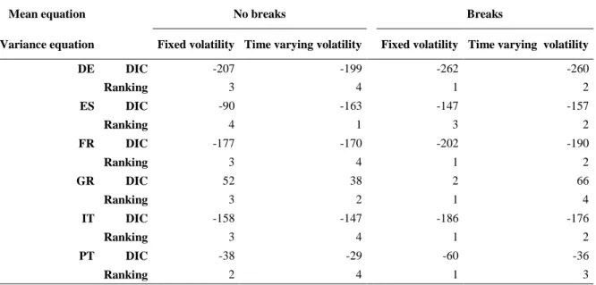
This section presents the Bayesian estimates of the different models. We first estimate a model with constant parameters and volatility using data spanning from February 2003 to October 2014. Then, we run structural break tests. They indicate that the parameters are unlikely to remain constant over the whole time period, implying that the long-run relationship seems to have changed during the crises. In a third section, we estimate models allowing the parameters of the mean equation to vary over time. We provide results for models with constant or time-varying variances. The fourth subsection is devoted to a sensitivity analysis consisting of the examination of the changes in the results due to the use of alternative measures of banks’ marginal cost in the model. The models are compared in the fifth sub-section with the Deviance Information Criterion (Spiegelhalter et al. (2002)). In a sixth subsection, we provide the contribution of the observed variables and of the errors to the total variance. To provide an order of magnitude of the change in the equilibrium, we simulate interest rates under the equilibrium prevailing before the financial crisis. In a seventh subsection, we focus on the heterogeneity of the development in the pass-through within each country and across borrowers’ sizes. We hence investigate whether changes in the pass-through have impacted more specifically small or
large firms. We assess the sensitivity of the results to the breakdates in the eighth section. The last section is dedicated to VAR analysis.
4.1. Models with a unique long-run relationship
Bayesian estimates of the main parameters of the error-correction model, assuming a variance constant over time, are reported in Table 3 (the whole set of estimates is in Table A.1 in the Appendix). The short-term pass-through is fairly high; it ranges from 0.49 to 0.79 for all countries except Portugal (0.23). Under this model, the pass-through seems complete on the long-run for all countries. However, the confidence intervals are very large for Spain and the estimates are very inaccurate. In this case, we cannot, on the opposite, reject the assumption of no long-term pass-through. As a consequence, the mean adjustment duration before a change in banks’ marginal cost is fully passed to bank lending rates is especially high for Spain (about 2 years and a half). For the other countries, the estimates are in line with what is reported in Sander and Kleimeier (2004), de Bondt (2005) or Kleimeier and Sander (2006).
Table 3: Estimates of the error-correction model with a single equilibrium and a constant variance Immediate pass-thr. Long-term pass-thr. Complete
pass-thr. Adjustment coef. Duration MC
1
Mean 2.5% 97.5% Mean 2.5% 97.5% Mean 2.5% 97.5% Mean
DE 0.79 0.66 0.93 0.90 0.81 0.98 No -0.22 -0.34 -0.10 1 ES 0.62 0.42 0.80 0.81 0.00 2.22 Yes -0.04 -0.09 0.00 20 FR 0.89 0.75 1.02 0.99 0.95 1.03 Yes -0.48 -0.63 -0.35 0 GR 0.49 0.23 0.78 0.69 0.13 1.08 Yes -0.14 -0.24 -0.03 6 IT 0.55 0.44 0.68 0.94 0.75 1.14 Yes -0.16 -0.25 -0.07 3 PT 0.23 0.08 0.38 0.79 0.56 1.05 Yes -0.17 -0.26 -0.09 5
Note: Cost of bank resources is measured by the rate on new deposits with a maturity lesser than one year. Estimated coefficients in bold are significant at 5% level. Durations are in months.
Figure 4 displays the squared residuals of the error-correction model with a constant variance. Since the residual is mean zero, the squared residual is an approximation of the contemporaneous variance. Whereas pure randomness can fully explain some clustering in the errors, the general patterns accord with economic intuition. As regards Greece, Spain and to a lesser extent Portugal, shocks at the end of 2008 and after, are of a bigger magnitude than those before. This raises doubts on the ability of the model with a constant variance to fit the data after the financial crisis for countries with sovereign debt concerns.
Figure 4: Squared residuals of the error-correction model with a constant variance and without breaks in the parameters (February 2003-October 2014)
4.2. Tests for structural breaks
We investigate here the assumption of breaks in bank lending rate dynamics in the different countries. We first perform various tests for structural change in the linear regression model in order to date the breaks.
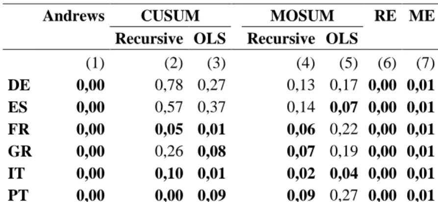
We test for the null hypothesis that parameters in equation (0.1) remain constant over time. Table 4 reports the p-values corresponding to the seven tests realised. At least five of them conclude that the parameters of the standard error-correction model vary over time for France, Greece, Italy and Portugal. With only three rejections of the null hypothesis over seven tests, Germany is the country for which we have the weaker evidences of change in the pass-through relationship. These results support the view that there are breaks in the pass-through mechanism.
Table 4: P-values of the tests for structural breaks
Andrews CUSUM MOSUM RE ME
Recursive OLS Recursive OLS
(1) (2) (3) (4) (5) (6) (7) DE 0,00 0,78 0,27 0,13 0,17 0,00 0,01 ES 0,00 0,57 0,37 0,14 0,07 0,00 0,01 FR 0,00 0,05 0,01 0,06 0,22 0,00 0,01 GR 0,00 0,26 0,08 0,07 0,19 0,00 0,01 IT 0,00 0,10 0,01 0,02 0,04 0,00 0,01 PT 0,00 0,00 0,09 0,09 0,27 0,00 0,01
Note: P-values in bold are significant at the 10% level. Column (1) refers to the extension of the Chow test to an unknown change point provided by Andrews (1993). Tests in columns (2) and (3) are based on the cumulative sums of recursive residuals (Brown et al., (1975)) and the cumulative sum of OLS standardized residuals (Ploberger and Krämer, (1992)). Column (4) and (5) display the results of tests based on the moving sums of residual (Chu et al., (1995)). Column (6) and (7) test for differences in the when they are estimated recursively with a growing number of observations or with a moving window, relative to estimates based on the whole sample (Ploberger et al., (1989), Chu et al., (1995)).
We now try to date the breaks. To this aim, we use the test pioneered by Bai and Perron (1998).10 The
test analyses the residuals from Equation (0.1), that is the model with constant parameters and variance, to assess the stability of the parameters over time and to date potential breakpoints. Table 5 reports the estimated breakdates and their confidence intervals at the 5% level.
Table 5: Estimated breakdates and their confidence intervals
First breakdate Second breakdate
Mean 2.5% 97.5% Mean 2.5% 97.5% DE 2009-02 2008-08 2009-05 2011-12 2011-11 2012-08 ES 2010-06 2010-01 2010-08 2013-03 2012-09 2013-04 FR 2006-01 2005-12 2006-06 GR 2011-12 2011-02 2012-01 IT 2008-10 2008-07 2008-11 2010-05 2010-02 2010-08 PT 2009-01 2008-12 2009-02
Note: Breakdates are simultaneously estimated with Bai and Perron (1998) test for multiple breaks.
10 We use the Bai and Perron (1998) test implemented in the library ‘strucchange’ (Zeileis et al. (2002)) for the R software (R Core Team
The test leads to one or two breakdates per country. Their main characteristics are the following. A first breakdate is identified between July 2008 and May 2009 for Germany, Italy and Portugal. It is followed by another one in the first half of 2010 in Italy and Spain. A last breakdate presumably occurred around December 2011 as regards Germany and Greece. The set of breakdates therefore highlights three sub-periods, comprising the most acute phase of the financial crisis, the beginning of the European sovereign debt crisis and finally the policy measures that stop the fragmentation of the Euro area. It is worth noting that the application of a test for dating structural breaks to a simple pass-through specification leads to results that could have been anticipated on economic grounds only. To identify accurately the breakdates, we look for the monetary and financial events large enough to impact all the six countries. In line with the tests, we focus on the events that occur between July 2008 and May 2009, during the first half of 2010 and near December 2011. The major event of the first period is clearly Lehman Brothers’ failure which triggered financial turmoil. We can see from Figure 2 that spreads start to increase immediately, in contradiction with the assumption of a permanent pass-through mechanism. We therefore set a first breakdate in September 2008. The first half of 2010 is related to the beginning of the sovereign debt crisis. The Greek budget deficit was subject to large corrections in October 2009. We can see from Figure 2 that spreads are quite stable over the year 2009 and start to vary again in early 2010. We therefore set the second breakdate in January 2010. During the first quarter of 2010, the Greek government implemented several measures to cut the deficit (cuts in the public sector, increase in taxes, etc.). By April 2010, the Greek sovereign requested assistance from the European Union and the IMF. A few days later, Standard and Poor’s rating of Greek sovereign debt has been downgraded to BB+. Several monetary policy measures have been designed during the sovereign debt crisis to bring back depth and liquidity in markets, so as to restore the transmission of the monetary policy. We only mention in the next lines the most significant measures.11 In May 2010, the ECB initiated the Securities Market Programme (SMP). Within this
program, the ECB and other central banks could intervene directly in the euro area debt market, by buying from banks the securities, whether public or private, usually accepted as collateral. On December 2011, the ECB announced and implemented a program providing 3 year loans with a 1% interest rate to European banks. We can see from Figure 2 that the spread varies a lot in Greece and Portugal at the very beginning of 2012. Therefore, we set the third breakpoint in January 2012. A second round of Long Term Refinancing Operations (LTROs) has been implemented on February 2012, providing banks with further 529 billion euro to 800 banks. The last SMP purchases took place in February 2012.
To sum up, structural break tests indicate change in the parameters over time. Using both statistical tests and economic stylised facts, we set the breakdates in September 2008, January 2010 and January 2012. For the sake of comparability, the breakdates are common to all the countries. In the remainder of the paper, we consider that the full sample is made up of sub-periods over which the parameters are constant. The parameters may take different values from one period to the other according to Equation (1.2). Note that we do not restrict the parameters to differ from one period to the other. A model with parameters constant over time is therefore nested within our most general specification.
4.3. Models with multiple long-run relationships
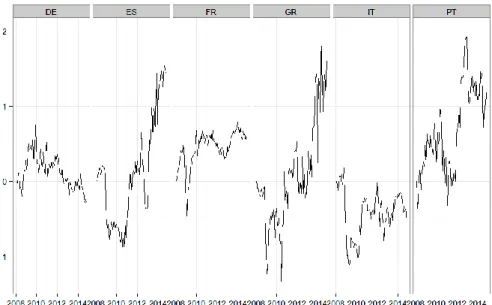
The pass-through model considered in the previous subsection supposes that the parameters of Equation (0.1) and the variance of the error terms are constant over time. The examination of the squared residuals and the test for structural breaks show those two assumptions are questionable. The economic intuition supports this view, as we can expect both banks’ interest rate setting and the unexpected shocks on the interest rates dynamic to be of greater magnitude during crises. Therefore, it suggests that first, the parameters governing the long-run relationship are subject to variations since the beginning of the financial crisis and second, the variance of the unexpected shocks vary over time. We consider in the following sections the results of models with parameters varying over time intervals, along with a constant or time-varying variance. The results regarding the main parameters
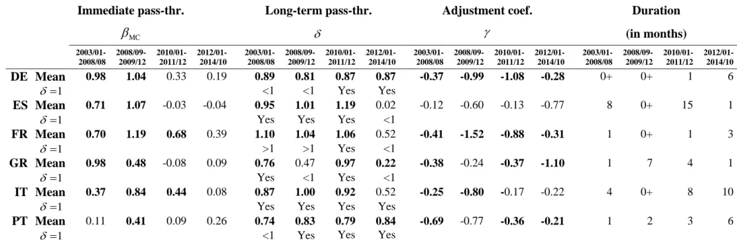
estimated assuming a constant variance, are reported in Table 6 and those assuming a stochastic volatility are in Table 7. Detailed results, including estimated parameters of the stochastic volatility equation, are in the Appendix (Tables A.3 and A.4).
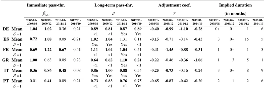
We find that the short-run pass-through significantly decreases during the sovereign debt crisis for Germany and Spain (Table A.3 in the Appendix). While positive significant in all countries before the sovereign debt crisis, it turns to be lower in all countries and no longer significant in most of them after January 2010. This is an unprecedented event in the years 2000’.
The long-term pass-through is close to 1 for most countries and time periods before January 2012. Therefore, the financial and sovereign debt crises did not alter the long-term relationship between the banks’ cost on resources and the price of new loans. On the contrary, it is after the LTROs and the most acute phase of the sovereign debt crisis that the long-term pass-through is significantly weakened in Greece and Spain. The results also suggest a decrease in France and Italy.
The adjustment coefficients are mostly and significantly negative. During the financial crisis, they significantly decrease for France and Germany, leading to quicker adjustments in the interest rates in these countries.
Recall that the use of the error correction models is motivated by cointegrating relationship between bank lending rates and their marginal cost (Phillips and Loretan (1991) and Hofmann and Mizen, (2004)). Both series share a common stochastic drift when
differs from zero, which is often not the case for Spain. Hence, we cannot completely exclude that the rate on new deposits is not an appropriate measure of the marginal cost faced by banks in Spain.The durations for the adjustments after a shock to be completed show a pattern common to all countries. It decreases during the financial crisis. Hence, the sharp decline in the rates managed by the monetary authorities has been followed by a decrease in the rates on new deposits and nearly simultaneously by a decline in the rate on new loans in all countries except Greece. After January 2010, however, the adjustment durations increase up to levels higher than those observed prior to the financial crisis. Hence, the results point to a slowdown in the transmission of change in bank marginal cost to the rate on new loans after the onset of the sovereign debt crisis.
We test for the stationarity of the elements on the right hand side of equation (0.2). We reject the assumption of explosive paths for the changes in the new loans rates, the long-term component and the residuals. Had we used variables not centered on their means computed over the different time periods, the long-term component would be stationary only up to a constant.