HAL Id: hal-01361482
https://hal.archives-ouvertes.fr/hal-01361482v3
Submitted on 7 Aug 2017
HAL is a multi-disciplinary open access
archive for the deposit and dissemination of
sci-entific research documents, whether they are
pub-lished or not. The documents may come from
teaching and research institutions in France or
abroad, or from public or private research centers.
L’archive ouverte pluridisciplinaire HAL, est
destinée au dépôt et à la diffusion de documents
scientifiques de niveau recherche, publiés ou non,
émanant des établissements d’enseignement et de
recherche français ou étrangers, des laboratoires
publics ou privés.
Antimagic Labelling Conjecture
Julien Bensmail, Mohammed Senhaji, Kasper Szabo Lyngsie
To cite this version:
Julien Bensmail, Mohammed Senhaji, Kasper Szabo Lyngsie. On a combination of the 1-2-3
Con-jecture and the Antimagic Labelling ConCon-jecture. Discrete Mathematics and Theoretical Computer
Science, DMTCS, 2017, 19 (1). �hal-01361482v3�
On a combination of the 1-2-3 Conjecture and
the Antimagic Labelling Conjecture
Julien Bensmail
1Mohammed Senhaji
2Kasper Szabo Lyngsie
3 1I3S/INRIA, Université Nice-Sophia-Antipolis, France
2
LaBRI, Université de Bordeaux, France
3
Technical University of Denmark, Denmark
received 16thOct. 2016, revised 6thApr. 2017, accepted 5thJuly 2017.
This paper is dedicated to studying the following question: Is it always possible to injectively assign the weights 1, ..., |E(G)| to the edges of any given graph G (with no component isomorphic to K2) so that every two adjacent
vertices of G get distinguished by their sums of incident weights? One may see this question as a combination of the well-known 1-2-3 Conjecture and the Antimagic Labelling Conjecture.
Throughout this paper, we exhibit evidence that this question might be true. Benefiting from the investigations on the Antimagic Labelling Conjecture, we first point out that several classes of graphs, such as regular graphs, indeed admit such assignments. We then show that trees also do, answering a recent conjecture of Arumugam, Premalatha, Baˇca and Semaniˇcová-Feˇnovˇcíková. Towards a general answer to the question above, we then prove that claimed assignments can be constructed for any graph, provided we are allowed to use some number of additional edge weights. For some classes of sparse graphs, namely 2-degenerate graphs and graphs with maximum average degree 3, we show that only a small (constant) number of such additional weights suffices.
Keywords: 1-2-3 Conjecture, Antimagic Labelling Conjecture, equitable edge-weightings
1
Introduction
In order to present our investigations in this paper, as well as our motivations, we first need to introduce a few particular graph concepts and notions. We refer the reader to textbooks on graph theory for more details on any standard notion or terminology not introduced herein.
Given a (undirected, simple, loopless) graph G and a set W of weights, by a W -edge-weighting of G we mean an edge-weighting with weights from W . For any k ≥ 1, a k-edge-weighting is a {1, ..., k}-edge-weighting. Given an edge-weighting w of G, one can compute, for every vertex v of G, the sum σ(v) (or σw(v) when more precision is needed) of weights assigned by w to the edges incident to v. That is,
σw(v) :=
X
u∈N (v)
w(vu)
for every vertex v of G. In case we have σw(u) 6= σw(v) for every edge uv of G, we call w
neighbour-sum-distinguishing. It can be observed that every graph with no connected component isomorphic to K2
admits neighbour-sum-distinguishing edge-weightings using sufficiently large weights. In the context of the current investigations, when speaking of a nice graph we mean a graph with no connected component isomorphic to K2. For a nice graph G, it hence makes sense to study the smallest k such that G admits a
neighbour-sum-distinguishing k-edge-weighting. We denote this chromatic parameter by χeΣ(G).
Throughout this paper, we deal with edge-weightings that are not only neighbour-sum-distinguishing but also do not assign any edge weight more than once. We say that such edge-weightings are edge-injective. Still under the assumption that G is a nice graph, we denote by χe,1Σ (G) the smallest k such that G admits an edge-injective neighbour-sum-distinguishing k-edge-weighting.
In this paper, we consider the following conjecture. Our motivations for studying this conjecture, as well as our evidences to suspect that it might be true, are described below.
Conjecture 1.1. For every nice graph G, we have χe,1Σ (G) = |E(G)|.
By the edge-injectivity property, we note that |E(G)| is a lower bound on χe,1Σ (G) for every nice graph G. Conjecture 1.1, in brief words, hence asks whether, for every nice graph G, we can bijectively assign weights 1, ..., |E(G)| to the edges of G so that no two adjacent vertices of G get the same value of σ.
Conjecture 1.1 is related to the well-known 1-2-3 Conjecture, raised in 2004 by Karo´nski et al. (2004), which states the following.
1-2-3 Conjecture. For every nice graph G, we have χe
Σ(G) ≤ 3.
Many aspects of the 1-2-3 Conjecture have been studied in literature. For an overview of those considered aspects, we refer the interested reader to the wide survey by Seamone (2012), which is dedicated to this topic. Our investigations in this paper are mostly related to a recent equitable variant of the 1-2-3 Conjecture that was considered by Baudon et al. (2017). In this variant, the authors studied, for some families of nice graphs, the existence of neighbour-sum-distinguishing edge-weightings being equitable, i.e. in which any two distinct edge weights are assigned about the same number of times (being equal, or differing by 1). In particular, they introduced and studied, for any given graph G, the chromatic parameter denoted by χe
Σ(G)
being the smallest maximal weight in an equitable neighbour-sum-distinguishing edge-weighting of G. In brief words, they proved that, at least for particular common classes of nice graphs (such as complete graphs and some bipartite graphs), the two parameters χe
Σand χeΣare equal except for a few exceptions.
Despite their results, Baudon et al. did not dare addressing a general conjecture on how should χe Σbehave
in general, or compared to χe
Σfor a given nice graph. In particular, it does not seem obvious how big χeΣ
can be, neither whether this parameter can be arbitrarily large. This is one of our motivations for study-ing edge-injective neighbour-sum-diststudy-inguishstudy-ing edge-weightstudy-ings, as an edge-injective edge-weightstudy-ing is always equitable. Thus, χe
Σ(G) ≤ χ e,1
Σ (G) holds for every nice graph G. Hence, attacking Conjecture 1.1
can be regarded as a way to get progress towards all those questions.
Our second motivation for considering Conjecture 1.1 is that edge-injective neighbour-sum-distinguishing edge-weightings can be regarded as a weaker notion of well-known antimagic labellings. Formally, using our own terminology, an antimagic labelling w of a graph G is an edge-injective |E(G)|-edge-weighting of G for which σwis injective, i.e. all vertices of G get a distinct sum of incident weights by w. We say that
G is antimagic if it admits an antimagic labelling. Many lines of research concerning antimagic labellings can be found in literature, most of which are related to the following conjecture addressed by Hartsfield and Ringel (1990).
Antimagic Labelling Conjecture. Every nice connected graph is antimagic.
Despite lots of efforts (refer to the dynamic survey by Gallian (1997) for an in-depth summary of the vast and rich literature on this topic), the Antimagic Labelling Conjecture is still open in general, even for common classes of graphs such as nice trees. Conjecture 1.1, which is clearly much weaker than the Antimagic Labelling Conjecture, as the distinction condition here only concerns the adjacent vertices, hence sounds as a much easier challenge to us, in particular concerning classes of nice graphs that are not known to be antimagic.
Hence, every antimagic graph G agrees with Conjecture 1.1, implying, as described earlier, that χe
Σ(G) ≤ χ e,1
Σ (G) = |E(G)|
holds, thus providing an upper bound on χe
Σ(G) for G. This is of interest as several classes of graphs, such
as nice regular graphs and nice complete partite graphs, are known to be antimagic, as reported by Gallian (1997). Let us here further mention the works of Bérci et al. (2015), and of Cranston et al. (2015), who led to the verification of the Antimagic Labelling Conjecture for nice regular graphs, and whose some proof techniques partly inspired some used in the current paper. Conversely, proving that a graph G verifies χe,1Σ (G) = |E(G)| and agrees with Conjecture 1.1 is similar to proving that, in some sense, G is “locally antimagic”.
Conjecture 1.1 can essentially be considered as a combination of the 1-2-3 Conjecture and the Antimagic Labelling Conjecture, as the notions behind it have flavours of both conjectures. As described earlier, prov-ing Conjecture 1.1 for some classes of graphs has, to some extent, consequences on the 1-2-3 Conjecture and the Antimagic Labelling Conjecture, or at least on variants of these conjectures.
Our work in this paper, is focused on both proving Conjecture 1.1 for particular classes of nice graphs, and providing upper bounds on χe,1Σ for some classes of nice graphs. This paper is organized as follows. Tools
and preliminary results we use throughout are introduced in Section 2. After that, we start off by providing support to Conjecture 1.1 in Section 3, essentially by showing and pointing out that the conjecture holds for some classes of graphs, such as nice trees and regular graphs. Towards Conjecture 1.1, we then provide, in Section 4, general weaker upper bounds on χe,1Σ . These bounds are then improved for some classes of nice sparse graphs in Section 5. These classes include nice graphs with maximum average degree at most 3 and nice 2-degenerate graphs. Concluding comments are gathered in Section 6.
Remark: During the review process, we have been notified that a paper introducing the notion of “locally antimatic graphs”, written by Arumugam et al. (2017), appeared online. That paper and the current one consider different aspects of this notion. Namely, Arumugam et al. focused on the smallest number of colour sums by an edge-injective neighbour-sum-distinguishing |E(G)|-edge-weighting. In particular, our Theorem 3.3 on trees answers positively to Conjecture 2.3 raised in Arumugam et al. (2017).
2
Preliminary remarks and results
In this section, we introduce several observations that will be of some use in the next sections. Con-jecture 1.1 is mainly about k-edge-weightings; however, to lighten some proofs, we will rather focus on edge-weightings assigning strictly positive weights only. The reader should keep this detail in mind.
We start off by pointing out a few situations in which, for a given edge uv of any graph G, we necessarily get σ(u) 6= σ(v) by an edge-injective edge-weighting of G. We omit a formal proof as it is easily seen that these claims are true. We note that the third item is more general, as it implies the other two.
Observation 2.1. Let G be a graph, and w be an edge-injective edge-weighting of G. Then, for every edge uv of G, we have σ(u) 6= σ(v) in any of the following situations:
1. d(u) = 1 and d(v) ≥ 2; 2. d(u) = d(v) = 2; 3. d(u) ≥ d(v) and
min {w(uv0) : v0 ∈ N (u) \ {v}} ≥ max {w(vu0) : u0∈ N (v) \ {u}} .
We now observe that to be able to successfully extend a partial neighbour-sum-distinguishing edge-weighting to an edge, we need to have sufficiently distinct weights in hand for that purpose.
Observation 2.2. Let G be a graph, uv be an edge of G, and w be a neighbour-sum-distinguishing edge-weighting ofG − {uv} such that σ(u) 6= σ(v). Then w can be successfully extended to uv, provided we have a setW of at least d(u) + d(v) − 1 distinct strictly positive weights that can be assigned to uv. Proof: We note that w currently must satisfy σ(u) 6= σ(v), as, otherwise, no matter what weight we assign to uv, we would eventually get σw(u) = σw(v). Under that assumption, we note that weighting uv with any
weight completely determines the value of both σw(u) and σw(v). The value of σw(u) eventually has to be
different from the sums of weights incident to the d(u) − 1 neighbours of u different from v. Similarly, the value of σw(v) eventually has to be different from the sums of weights incident to the d(v) − 1 neighbours
of v different from u. The neighbours of u and v hence forbid us from assigning at most d(u) + d(v) − 2 possible distinct weights to uv. Now, since weighting uv with distinct weights results in distinct values of σw(u) and σw(v), it should be clear that we can find a correct weight for uv in W , provided W includes at
least d(u) + d(v) − 1 distinct weights.
Throughout this paper, several of the proofs consist in deleting two adjacent edges vu1and vu2from G,
edge-weighting the remaining graph, and correctly extending the weighting to vu1and vu2. In this regard,
we will often refer to the following result, which is about the number of weights that are sufficient to weight vu1and vu2.
Observation 2.3. Let G be a graph having two adjacent edges vu1andvu2such thatG0:= G−{vu1, vu2}
admits a neighbour-sum-distinguishing edge-weightingwG0. Assume further thatdG(u1) ≥ dG(u2), and
set
µ := (dG(u1) + 1) + max {0, dG(v) + dG(u2) − dG(u1) − 1} .
Then, assuming we have a setW of at least µ distinct strictly positive weights, we can extend wG0 to a
Proof: We extend wG0 to a neighbour-sum-distinguishing edge-weighting wG of G by first assigning a
weight of W to vu1, and then assigning a distinct weight to vu2. We determine, in this proof, the
small-est number µ of weights that W should contain so that this strategy has sufficiently many weights to be successfully applied.
We note that extending wG0 to vu1 completely determines the value of σw
G(u1), while the value of
σwG(v) is not determined until vu2is also weighted. Hence, when first weighting vu1, we mainly have to
make sure that σwG(u1) does not get equal to the sum of weights incident to a neighbour of u1different
from v. Also, we should make sure that σwG0(v)+wG(vu1) does not get equal to σwG0(u2), as otherwise we
would necessarily get σwG(v) = σwG(u2) no matter how we weight vu2. There are hence dG(u1) conflicts
to take into account when weighting vu1. Provided W includes at least dG(u1) + 1 distinct weights, we can
hence weight vu1correctly, i.e. so that we avoid all conflicts mentioned above, with one weight from W ,
since assigning different weights to vu1alters σwG(u1) in distinct ways.
Now assume vu1has been weighted with the additional property that σwG0(v) + wG(vu1) 6= σwG0(u2).
Since that property holds, Observation 2.2 tells us that we can correctly extend wG0 to vu2provided W \
{wG(vu1)} includes at least dG(v) + dG(u2) − 1 distinct weights. We hence need W \ {wG(vu1)} to
include that many distinct weights.
As explained above, W necessarily includes at least dG(u1) weights that were not assigned to vu1.
Hence, to make sure, after weighting vu1, that W still includes at least dG(v) + dG(u2) − 1 distinct weights,
we need W to include at least
(dG(v) + dG(u2) − 1) − dG(u1)
other weights. This quantity can be negative, as, notably, vu1 may need a lot of weights to be weighted.
Hence
µ = (dG(u1) + 1) + max {0, dG(v) + dG(u2) − dG(u1) − 1} ,
as claimed, and, under the assumption that W has size µ, we can achieve the extension of wG0 to G as
described earlier.
In our proofs, we will also use the fact that, in some situations, pendant edges can easily be weighted assuming we are provided enough distinct weights.
Observation 2.4. Let G be a graph having a pendant edge vu, where u is the degree-1 vertex, such that G0:= G−{uv} admits a neighbour-sum-distinguishing edge-weighting wG0. Then, assuming we have a set
W of at least dG(v) distinct strictly positive weights, we can extend wG0 to a neighbour-sum-distinguishing
edge-weighting ofG by assigning a weight of W to vu.
Proof: Following Observation 2.1, when extending wG0 to vu, we do not have to care whether σ(u) gets
equal to σ(v). We thus just have to make sure that σ(v) does not get equal to the sum of weights incident to one of its neighbours in G0. Recall that assigning distinct weights to vu results in different sums as σ(v). Therefore, since v has dG(v) − 1 neighbours in G0while W has size at least dG(v), there is necessarily a
weight in W that can be assigned to vu such that no conflict is created. An extension of wG0 to G hence
exists.
3
Classes of graphs agreeing with Conjecture 1.1
As mentioned in Section 1, we directly benefit, in the context of Conjecture 1.1, from the investigations on antimagic labellings, as antimagic graphs verify Conjecture 1.1. Following the survey by Gallian (1997), the following classes of nice graphs hence agree with Conjecture 1.1.
Theorem 3.1. The classes of known antimagic graphs notably include: • nice paths (Hartsfield, Ringel Hartsfield and Ringel (1990)), • wheels (Hartsfield, Ringel Hartsfield and Ringel (1990)), • nice regular graphs (Bérci, Bernáth, Vizer Bérci et al. (2015)),
• nice complete partite graphs (Alon, Kaplan, Lev, Roditty, Yuster Alon et al. (2004)). Consequently, every of these graphsG verifies χe,1Σ (G) = |E(G)|.
When it comes to nice graphs with maximum degree 2, it is easily seen, as we are assigning strictly positive weights only, that any edge-injective edge-weighting is neighbour-sum-distinguishing. Disjoint unions of nice paths and cycles hence agree with Conjecture 1.1.
Observation 3.2. Let G be a nice graph with ∆(G) = 2. Then any edge-injective edge-weighting of G is neighbour-sum-distinguishing.
One of the main lines of research concerning antimagic labellings is to determine whether nice trees are all antimagic. In the following result, we prove that this question can be answered positively when relaxed to edge-injective neighbour-sum-distinguishing edge-weightings. We actually prove a stronger statement that will be useful in the next sections.
Theorem 3.3. Let F be a nice forest. Then, for every set W of |E(F )| distinct strictly positive weights, there exists an edge-injective neighbour-sum-distinguishingW -edge-weighting of F . In particular, we have χe,1Σ (F ) = |E(F )|.
Proof: If ∆(F ) = 2, then the result follows from Observation 3.2. So the claim holds whenever F has size 2. Assume now that the claim is false, and let F be a counterexample that is minimum in terms of nF+ mF, where nF := |V (F )| and mF := |E(F )|. By the remark above, we have mF ≥ 3. Let W :=
{α1, ..., αmF} be a set of distinct strictly positive integers such that F does not admit an edge-injective
neighbour-sum-distinguishing W -edge-weighting. Free to relabel the weights in W , we may suppose that α1 < ... < αmF. Due to the minimality of F , we may assume that F is a tree (as otherwise we could
invoke the induction hypothesis). Furthermore, we may assume that F has maximum degree at least 3 (at otherwise Observation 3.2 would apply).
We now successively show that F , because it is a counterexample to the claim, cannot contain certain structures, until we reach the point where F is shown to not exist at all, a contradiction. In particular, we focus on the length of the pendant paths of F , where a pendant path of F is a maximal path vk...v1, where
k ≥ 2, such that d(vk) ≥ 3, d(vk−1) = ... = d(v2) = 2, and d(v1) = 1. In the case where k = 2, we note
that the pendant path is a pendant edge, in which case vk = v2and we have d(v2) ≥ 3. Since ∆(F ) ≥ 3,
there are at least three pendant paths in F .
We start off by showing that the pendant paths of F all have length at most 2. Claim 3.4. Every pendant path of F has length at most 2.
Proof: Assume F has a pendant path P := vk...v1with k ≥ 4, where d(vk) ≥ 3. In this case, let F0 :=
F − {vk−1vk−2, ..., v2v1} be the tree obtained by removing, from F , all edges of P but the one incident
to vk. Clearly, F0is nice and, due to the minimality of F , there exists an edge-injective
neighbour-sum-distinguishing {α1, ..., αmF 0}-edge-weighting wF0 of F0, where mF0 := |E(F0)|. To prove that the claim
holds, we have to prove that we can extend wF0 to the edges vk−1vk−2, ..., v2v1, hence to F , using weights
αmF 0+1, ..., αmF, so that we get an edge-injective neighbour-sum-distinguishing W -edge-weighting of F ,
a contradiction.
Due to the length of P , we have |{αmF 0+1, ..., αmF}| ≥ 2. When weighting the edges vk−1vk−2, ..., v2v1,
we note that we cannot create any sum conflicts involving any two consecutive vertices in {v1, ..., vk−1}.
That is, the incident sums of any two of these vertices can never get equal. This is according to Observa-tion 2.1 since we are assigning weights injectively. Hence, when extending wF0, we just have to make sure
that σ(vk−1) gets different from σ(vk), which is possible as we have at least two distinct edge weights to
work with. So we can assign a weight to vk−1vk−2which avoids that conflict, and then arbitrarily extend
the weighting to the edges vk−2vk−3, ..., v2v1. This yields an edge-injective neighbour-sum-distinguishing
W -edge-weighting of F .
Now designate a vertex r with degree at least 3 of F as being the root of F . This naturally defines, in the usual way, an orientation of F from its root to its leaves. For every vertex v of F , the father f (v) of v is the neighbour of v which is the closest from r (if any). Conversely, the descendants of v are all vertices, different from v, in the subtree of F rooted at v (if any). We note that r has no father, while the leaves of F have no descendants. The descendants of v adjacent to v (if any) are called its children.
A multifather v of F is a vertex with degree at least 3, i.e. having at least two children. In case all descendants of v have degree at most 2, we call v a last multifather of F . In other words, a last multifather is a vertex with at least two pendant paths attached. Since ∆(F ) ≥ 3, there are last multifathers in F .
To further study the structure of F , we now prove properties of its last multifathers, still under the as-sumption that F is rooted at a vertex r with degree at least 3.
Claim 3.5. Vertex r is not a last multifather.
Proof: Assume the contrary. Then r is the only vertex with degree at least 3 of F . In other words, F is a subdivided star. Then it should be clear that assigning the weights αmF, αmF−1, ..., α1, following this
order, to the edges of F as they are encountered during a breadth-first search algorithm performed from r results in a neighbour-sum-distinguishing edge-weighting of F . To be convinced of this statement, one can e.g. refer to Observation 2.1.
Due to Claim 3.5, we may assume that the root r of F is not a last multifather. Then all last multifathers of F (there are some) are different from r, and hence have a father. We now refine Claim 3.4 to the following. Claim 3.6. Every pendant path attached to a last multifather of F has length 1.
Proof: Let v 6= r be a last multifather of F , and assume v is incident to pendant paths with length 2. We recall that all pendant paths attached to v have length at most 2 (Claim 3.4), and, since v is a last multifather, it is incident to at least two pendant paths. Let F0 be the tree obtained from F by removing all pendant paths attached to v. Because mF0 := |E(F0)| is smaller than mF, there exists an edge-injective
neighbour-sum-distinguishing {α1, ..., αmF 0}-edge-weighting wF0 of F0. For contradiction, we prove below that wF0
can be extended correctly to the pendant paths attached to v using the weights among {αmF 0+1, ..., αmF}
injectively.
Let b ≥ 1 be the number of pendant paths of length 2 attached to v in F , and let vx1y1, ..., vxbybdenote
those paths (so that the xi’s have degree 2 in F , while the yi’s have degree 1). Vertex v is also adjacent to
c ≥ 0 leaves xb+1, ..., xb+c, which are, in some sense, pendant paths of length 1. Since v is a multifather,
we recall that b + c = dF(v) − 1 ≥ 2.
We extend wF0 to the edges of the pendant paths attached to v in the following way. First, we injectively
arbitrarily assign the dF(v) − 1 weights in {αmF−dF(v)+2, ..., αmF} to the edges vx2, ..., vxb+c. After
that, we assign to the edge vx1one of the weights αmF−dF(v)+1or αmF−dF(v)chosen so that σwF(v) is
different from the sum of weights incident to f (v), the father of v, by wF0. We then assign to x1y1the one
weight of αmF−dF(v)+1or αmF−dF(v)not assigned to vx1. We note that no matter how we complete the
extension of wF0, eventually σw
F(v) will be strictly bigger than σwF(x1).
We finish the extension of wF0 to F by arbitrarily injectively assigning the remaining non-used smaller
weights to the edges x1y1, ..., xbyb. Because all the xi’s have degree 2 and the yi’s have degree 1, no conflict
may arise between those vertices (Observation 2.1). Furthermore, since the degree of v is larger than the degree of the xi’s, and the weights assigned to the vxi’s are bigger than the weights assigned to the xiyi’s
(with possibly the exception of vx1and x1y1, which we have discussed above), it should be clear that no
conflict may arise between v and the xi’s (again according to Observation 2.1). So we eventually get an
edge-injective neighbour-sum-distinguishing W -edge-weighting of F , a contradiction.
We finally study last multifathers of F being at maximum distance from r. We call these vertices the deepest last multifathersof F . From now on, we focus on a fixed deepest last multifather v∗of F , which we choose arbitrarily. In the upcoming proof, for any vertex v of F , we denote by Fv the subtree of F
rooted at v. Recall that all children of a last multifather are leaves (Claim 3.6).
Claim 3.7. Every last multifather v of Ff (v∗) is a child off (v∗). In other words, v is a deepest last
multifather ofF .
Proof: The claim follows from the fact that if there exists a descendant v 6= v∗of f (v∗) being at distance at least 2 from f (v∗), then v would, in F , be at greater distance from r than v∗is. This would contradict the fact that v∗is a deepest last multifather.
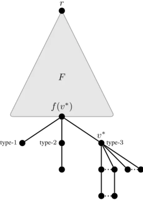
Recall that f (v∗) cannot be incident, in F , to a pendant path with length at least 3 (Claim 3.4). Hence, every child of f (v∗) is either a leaf (type-1), a degree-2 vertex adjacent to a leaf (type-2, i.e. the inner vertex of a pendant path with length 2), or a deepest last multifather (type-3). See Figure 1 for an illustration. Furthermore, we know that f (v∗) is adjacent to at least one type-3 vertex, which is v∗. In the following proof, we show that v∗is actually the only child of f (v∗) in F .
Claim 3.8. Vertex v∗is the only child off (v∗) in F .
Proof: Suppose the claim is false, and let v 6= v∗ be another child of f (v∗). Let x1and x2be two leaves
adjacent to v∗, which exist since v∗is a last multifather, and all pendant paths attached to v∗have length 1 (Claim 3.6).
F r
f (v∗)
type-1 type-2 type-3
v∗
Figure 1: Illustration of the three child types mentioned in the proof of Theorem 3.3.
Assume first that v is type-2 or type-3, or, in other words, that dF(v) ≥ 2. In that case, v is adjacent
to at least one leaf, say y. We here consider F0 := F − {vy, v∗x1, v∗x2}. Note that F0remains nice and
has fewer edges than F . Due to the minimality of F , there hence exists an edge-injective neighbour-sum-distinguishing {α1, ..., αmF 0}-edge-weighting wF0 of F0, where mF0 := |E(F0)|. We show
be-low that wF0 can be extended to the three removed edges with injectively using the three edge weights
αmF−2, αmF−1, αmF, yielding an edge-injective neighbour-sum-distinguishing W -edge-weighting wF of
F , a contradiction.
We first assign a weight to v∗x1 based on the conflicts that may happen when weighting vy. When
assigning any of the three weights to vy, the only problem which may occur, recall Observation 2.1, is that σwF(v) gets equal to σwF 0(f (v
∗)). If assigning one of the three weights α
mF−2, αmF−1, αmF to vy
indeed results in that conflict, we assign that weight to v∗x1. Otherwise, we assign any of the three weights
to v∗x1. In any case, no conflict may arise as σwF(v
∗) is still not determined.
We are now left with two weights, which we must assign to v∗x2and vy. Due to the choice of the weight
assigned to v∗x1, we note that no problem may occur when weighting vy. Hence, we just have to weight
v∗x2correctly and assign the remaining weight to vy. When weighting v∗x2, the only problem which may
occur, according to Observation 2.1, is that σwF(v
∗) gets equal to σ
wF 0(f (v∗)). But, since we have two
distinct weights to work with, one of them can be assigned to v∗x2so that this conflict is avoided. Thus
we can weight v∗x2correctly and eventually weight vy with the remaining weight, resulting in the claimed
wF.
We may now assume that all children, including v, of f (v∗) different from v∗ are type-1, i.e. leaves. The contradiction can then be obtained quite similarly as in the previous case but with setting F0 := F − {f (v∗)v, v∗x
1, v∗x2}. When weighting f (v∗)v, we have to make sure, if f (v∗) 6= r, that σwF(f (v ∗)) does
not get equal to σwF 0(f (f (v∗))). Note that if f (v∗) = r, then the situation is actually easier as there is
one less conflict to consider. If one of the three available weights αmF−2, αmF−1, αmF, when assigned to
f (v∗)v, yields a conflict involving f (v∗) and f (f (v∗)), then we assign that weight to v∗x1. Otherwise, we
assign any weight to v∗x1. This ensures that, when assigning any of the two remaining weights to f (v∗)v,
no conflict may involve f (v∗) and f (f (v∗)). We finally arbitrarily assign the two remaining weights to v∗x2and f (v∗)v. If this results in a neighbour-sum-distinguishing edge-weighting wF of F , then we are
done. Otherwise, it means that σwF(v ∗) = σ
wF(f (v
∗)). In that case, note that, because all assigned edge
weights are distinct, when swapping the values assigned to v∗x2and f (v∗)v by wF that conflict cannot
remain. Furthermore, according to the remarks above, we still do not create any sum conflict involving f (v∗) and f (f (v∗)). After the swapping operation wF hence gets neighbour-sum-distinguishing.
We are now ready to finish off the proof by showing that, under all information we have obtained, F actually admits an edge-injective neighbour-sum-distinguishing W -edge-weighting, a contradiction.
From Claim 3.8, we get that dF(f (v∗)) = 2, as v∗is not the root of F , so f (f (v∗)) exists. Let x1, ..., xk
be the k ≥ 2 leaves attached to v∗ in F , which exist since v∗ is a type-3 vertex. Now consider the tree F0:= F − {v∗x1, ..., v∗xk} with size mF0 := |E(F0)|. Due to the minimality of F , there exists an
edge-injective neighbour-sum-distinguishing {α1, ..., αmF 0}-edge-weighting wF0 of F0. We extend wF0 to the
k removed edges so that an edge-injective neighbour-sum-distinguishing W -edge-weighting wF of F is
obtained, a contradiction. To that aim, we arbitrarily injectively assign the weights αmF−k+1, ..., αmF to
the pendant edges v∗v1, ..., v∗vkattached to v∗. Recall that we cannot get sum conflicts involving v∗and the
vi’s according to Observation 2.1. Furthermore, we have dF(v∗) ≥ 3 while dF(f (v∗)) = 2 (Claim 3.8), and
we have used the k biggest weights of W to weight the edges incident to v∗. From this and Observation 2.1, we get that, necessarily, σwF(v
∗) > σ
wF 0(f (v∗)). So wF is neighbour-sum-distinguishing.
4
General upper bounds
Towards Conjecture 1.1, we start off by exhibiting, for any nice graph G, an upper bound on χe,1Σ (G) of the form k · |E(G)|, where k is a fixed constant.
It turns out, first, that some results towards the 1-2-3 Conjecture can be extended to the edge-injective context, hence yielding bounds to our context. This is in particular the case of the weighting algorithm by Kalkowski et al. (2010), which was designed to prove that χeΣ(G) ≤ 5 holds for every nice graph G. In very brief words, this algorithm initially assigns the list of weights {1, 2, 3, 4, 5} to every edge of G, which contains the possible weights that any edge can be assigned at any moment of the algorithm. The algorithm then linearly processes the vertices of G with possibly adjusting some incident edges weights (but staying in the list {1, 2, 3, 4, 5}) so that sum conflicts are avoided around any vertex considered during the course.
It is easy to check that this algorithm also works under the assumption that every edge of G is assigned a (possibly unique) list of five allowed consecutive weights {α − 2, α − 1, α, α + 1, α + 2}. In particular, when applied with non-intersecting such lists assigned to the edges, the algorithm yields an edge-injective neighbour-sum-distinguishing edge-weighting, as every edge weight can be assigned to at most one edge. So, applying the algorithm on a nice graph G with edges e0, ..., em−1 where each edge ei is assigned
the list {5i + 1, 5i + 2, 5i + 3, 5i + 4, 5i + 5} results in an edge-injective neighbour-sum-distinguishing (5 · |E(G)|)-edge-weighting of G. From this, we get that χe,1Σ (G) ≤ 5 · |E(G)| holds for every nice graph G.
The 5·|E(G)| bound on χe,1Σ (G) above can actually be improved down to 2·|E(G)| by means of a careful inductive proof scheme, which we describe in the following proof. We actually prove (here and further) a stronger statement to get rid of the non-connected cases.
Theorem 4.1. Let G be a nice graph. Then, for every set W of 2 · |E(G)| distinct strictly positive weights, there exists an edge-injective neighbour-sum-distinguishingW -edge-weighting of G. In particular, we have χe,1Σ (G) ≤ 2 · |E(G)|.
Proof: The proof is by induction on nG+ mG, where nG := |V (G)| and mG := |E(G)|. As it can easily
be checked that the claim is true for small values of nG+ mG, we proceed to the induction step. Consider
hence a value of nG+ mGsuch that the claim is true for smaller values of this sum.
We may assume that G is connected, as otherwise induction could be invoked on the different connected components of G. Set ∆ := ∆(G). Since we may assume that mG ≥ 4 and G is nice, we clearly have
∆ ≥ 2. We may even assume that ∆ ≥ 3, as otherwise G would admit an edge-injective neighbour-sum-distinguishing W -edge-weighting according to Observation 3.2. Consider any vertex v∗ of G verifying dG(v∗) = ∆ and denote by u1, ..., u∆the neighbours of v∗in G.
Set G0 := G − v∗. Note that G0may include connected components isomorphic to K2, and thus be not
nice. In this context, we say that a component of G0is empty if it has no edge, bad if it is isomorphic to K2,
and good otherwise. Basically, a bad component of G0is an edge to which v∗is joined in G: either v∗ is adjacent to the two ends of that edge, or v∗is adjacent to only one of the two ends.
If G0 does not have good components, then G is a connected graph whose only vertex with degree at least 3 is v∗ such that G0 consists of isolated vertices and isolated edges only. In particular, all ver-tices of G but v∗ have degree at most 2, and every degree-2 vertex ui adjacent to v∗ is either adjacent
to another degree-2 vertex uj adjacent to v∗, or adjacent to a degree-1 vertex. In such a situation,
weights α2mG, ..., α1, following this order, to the edges of G as they are encountered while performing
a breadth-first search algorithm from v∗, results in an injective neighbour-sum-distinguishing edge-weighting of G. This notably follows as a consequence of Observation 2.1.
Hence we may assume that G0has good connected components C1, C2, ... . Let H denote the union of
the Ci’s, and set mH := |E(H)|. Since the Ci’s are nice, so is H. Furthermore, we have that mH < mG.
According to the induction hypothesis, there hence exists an edge-injective neighbour-sum-distinguishing {α1, ..., α2mH}-edge-weighting wH of H. In order to get an edge-injective neighbour-sum-distinguishing
W -edge-weighting wG of G, we eventually need to extend wH to the remaining edges of G, i.e. to the
v∗ui’s and the edges of the bad components of G0.
To that aim, we restrict ourselves to injectively using weights among {α2mH+1, ..., α2mG}, i.e. we do
not use non-used weights among {α1, ..., α2mH}. Let u1, ..., ukdenote the neighbours of v
∗belonging to
good components of G. We start by injectively assigning weights to the edges v∗u1, ..., v∗ukusing ∆ + k
of the weights in {α2mG−(∆+k)+1, ..., α2mG}, without raising any sum conflict. This is possible for every
considered edge v∗ui, since each uihas degree at most ∆ − 1 in H and we have at least ∆ + k − (i − 1) ≥
∆ + 1 different available weights.
We are now left with weighting the edges of G belonging to the bad components, or being incident to the bad components (i.e. being incident to v∗). Assume there are m0 of them. Then we have mG =
mH+ k + m0, and, since k + m0≥ ∆, we have
2mG− (∆ + k) − 2mH = k + 2m0− ∆ ≥ m0.
The set {α2mH+1, ..., α2mG−(∆+k)} hence contains sufficiently many weights for weighting all of the m 0
remaining edges. To that aim, we assign the weights α2mG−(∆+k), ..., α2mH+1, following this order (i.e. in
decreasing order of magnitude), to these m0remaining edges as they are encountered during a breadth-first search algorithm performed from v∗.
It can easily be checked that, by the weighting scheme described above, the weights on the edges incident to v∗ are greater than all the weights on the edges incident to the neighbours of v∗. Hence, by Observa-tion 2.1, vertex v∗is distinguished from all its neighbours. By similar arguments, it can be checked that no sum conflicts can involve vertices of G − H, thus that the resulting edge-injective edge-weighting is neighbour-sum-distinguishing.
We now provide a second upper bound on χe,1Σ (G) of the form |E(G)| + k for every nice graph G. Here, our k is a small linear function of ∆(G), making the bound 1) mostly interesting in the context of nice graphs with bounded maximum degree, and 2) generally better than the bound in Theorem 4.1 (except in some cases to be discussed later). The proof scheme we employ here is different from the one used to prove Theorem 4.1.
Theorem 4.2. Let G be a nice graph. Then, for every set W of |E(G)| + 2∆(G) distinct strictly positive weights, there exists an edge-injective neighbour-sum-distinguishingW -edge-weighting of G. In particular, we haveχe,1Σ (G) ≤ |E(G)| + 2∆(G).
Proof: We may assume that G is connected. Set ∆ := ∆(G), and let n := |V (G)| and m := |E(G)| denote the order and size, respectively, of G. Also, set W := {α1, ..., αm+2∆} where α1< ... < αm+2∆.
First choose a vertex v∗with degree ∆ in G, and let T be a spanning tree of G including all edges incident to v∗. From T , we deduce a partition V0∪ ... ∪ Vkof V (G), where each part Viincludes the vertices of G
being at distance i from v∗in T . In particular, V0= {v∗}, and, for every vertex u in a part Viwith i 6= 0,
there is exactly one edge from u to Vi−1in T . We call this edge the private edge of u.
We now describe how to obtain an edge-injective neighbour-sum-distinguishing W -edge-weighting of G. We start by assigning the edge weights α1, ..., αm−(n−1)to the edges of E(G) \ E(T ) in an arbitrary
way. This leaves us with all edges of T to be weighted, which includes at least one incident (private) edge for every vertex different from v∗, and all edges incident to v∗. To weight these edges without creating any conflict, we will first consider all vertices of Vk and weight their private edges carefully, then do the same
for all vertices of Vk−1, and so on layer by layer until all edges of T are weighted. Fixing any ordering over
the vertices of Vk, ..., V1, this weighting scheme yields an ordering u1, ..., un−1in which the vertices are
considered (i.e. the |Vk| first ui’s belong to Vk, the |Vk−1| next ui’s belong to Vk−1, and so on; the |V1| last
ui’s belong to V1). We note that the private edges of the |V1| last ui’s go to v∗.
To extend the edge-injective neighbour-sum-distinguishing edge-weighting to the edges of T correctly, we consider the ui’s in order, and for each of these vertices, we weight its private edge in such a way that
no sum conflict arises. Assume we are currently dealing with vertex ui, meaning that all previous ui’s
have been correctly treated. If ui6∈ V1, then we assign to the private edge of uia non-used weight among
{αm−(n−1)+1, ..., αm} in such a way that σ(ui) gets different from the sums of the at most ∆ − 1 already
treated neighbours of ui. Note that, even for the last uinot in V1to be considered, the number of remaining
non-used weights in {αm−(n−1)+1, ..., αm} is at least ∆ + 1, so this weighting extension can be applied to
every vertex.
Now, if ui ∈ V1, then we apply the same strategy but with the weights among {αm+1, ..., αm+2∆}.
Again, even for un−1, note that this set includes at least ∆ + 1 non-used weights, so we can correctly
choose a weight for un−1v∗so that σ(un−1) gets different from the sums of the previously-treated vertices.
To finish off the proof, we note that, by that strategy, all edges incident to v∗ have been weighted with weights among {αm+1, ..., αm+2∆}. Since d(v∗) = ∆, by Observation 2.1 we get that σ(v∗) is eventually
strictly bigger than the sums incident to its neighbours.
As a concluding remark, we would like to point out that the 2 · |E(G)| bound from Theorem 4.1, can, in several situations, be better than the |E(G)| + 2∆(G) bound from Theorem 4.2. To be convinced of that statement, consider the class of graphs obtained by starting from any star with ∆ leaves u1, ..., u∆and
adding no more than ∆ − 1 edges joining pairs of vertices among {u1, ..., u∆}.
5
Refined bounds for particular classes of sparse graphs
We now improve the bounds in Section 4 to bounds of the form |E(G)| + k, where k is a small constant, for several classes of nice graphs G. Our weighting strategy here relies on removing some edges from G, then deducing a correct edge-weighting of the remaining graph, and extending that weighting to G. So that this weighting strategy applies, we focus on rather sparse graph classes with particular properties inherited by their subgraphs. In that respect, we give a special focus to nice 2-degenerate graphs, and nice graphs with maximum average degree at most 3. It is worth recalling that these graphs may have arbitrarily large maximum degree, so Theorem 4.2 does not provide the kind of bound we are here interested in.
Throughout this section, when speaking of a k-vertex, we mean a degree-k vertex. By a k−-vertex(resp. k+-vertex), we refer to a vertex with degree at most (resp. at least) k.
5.1
2-degenerate graphs
A graph G is said to be k-degenerate if every subgraph of G has a k−-vertex. In the next result, we focus on nice 2-degenerate graphs, and exhibit an upper bound on their value of χe,1Σ .
Theorem 5.1. Let G be a nice 2-degenerate graph. Then, for every set W of |E(G)| + 4 distinct strictly positive weights, there exists an edge-injective neighbour-sum-distinguishingW -edge-weighting of G. In particular, we haveχe,1Σ (G) ≤ |E(G)| + 4.
Proof: Assume the claim is false, and let G be a counterexample that is minimal in terms of nG+ mG,
where nG:= |V (G)| and mG:= |E(G)|. Set W := {α1, ..., αmG+4}. We show below that G cannot be a
counterexample, and thereby get a contradiction. This is done by showing that we can always remove some edges from G while keeping the graph nice, then deduce an edge-injective neighbour-sum-distinguishing {α1, ..., αmG0+4}-edge-weighting wG0 of the remaining graph G0, where mG0 := |E(G0)|, and finally
extend wG0 to get an edge-injective neighbour-sum-distinguishing W -edge-weighting wGof G.
We start by pointing out properties of G we may assume. Clearly, we may suppose that G is connected. According to Observation 3.2, we may also assume that ∆(G) ≥ 3, and, therefore, that mG ≥ 4, as
otherwise G would be a tree, in which case a weighting exists according to Theorem 3.3. We note as well that the 1-vertices of G must be adjacent to vertices with sufficiently large degree.
Claim 5.2. Every 1-vertex of G is adjacent to a 6+-vertex.
Proof: Assume for contradiction that G has a 1-vertex u adjacent to a 5−-vertex v. Let G0 := G − {uv}. Then G0 is 2-degenerate, and nice as otherwise G would be a path of length 2 (in which case
Theorem 3.3 applies). Thus G0 admits an edge-injective neighbour-sum-distinguishing {α1, ..., αmG0+4
}-edge-weighting wG0, where mG0 := mG− 1. According to Observation 2.4, we can correctly extend wG0
to uv, hence to G, since we have at least five distinct weights available for that. This is a contradiction. From Claim 5.2, we also deduce the following as a corollary.
Claim 5.3. G − {uv} is nice for every edge uv.
Proof: Let uv be an edge of G, and set G0:= G − {uv}. If dG(u) ≥ 3 and dG(v) ≥ 3, then G0is clearly
nice. Furthermore, if dG(u) = 1 or dG(v) = 1, then G0is nice by Claim 5.2.
Now assume that at least one of u and v has degree 2 in G. Without loss of generality, assume that dG(u) = 2, and let u0 be the neighbour of u different from v. By Claim 5.2 we have dG(v) ≥ 2 and
dG(u0) ≥ 2. If dG(v) ≥ 3, then clearly G0 is nice. So assume dG(v) = 2, and let v0 be the neighbour of v
different from u. Then, again by Claim 5.2, we have dG(v0) ≥ 2, and G0is nice.
As a consequence of Claim 5.3 and Observation 2.2, we immediately get the following. Claim 5.4. G has no edge uv with dG(u) + dG(v) ≤ 6.
We are now ready to start off the proof. Let S1denote the set of 2−-vertices of G, and set G1:= G − S1.
Since ∆(G) ≥ 3, graph G1has vertices. In particular, since G1is 2-degenerate, it has a 2−-vertex v. Let
us denote as d+(v) the number of neighbours, in G, of v in S
1. Then dG(v) = d+(v) + dG1(v).
First assume that d+(v) ≥ 3, and let v
1, v2, v3 be three neighbours of v in S1. We here consider
G0 := G − {vv1, vv2, vv3}. Note that G0 has to be nice, as otherwise G would have an edge
violat-ing Claim 5.4. Due to the minimality of G, and because G0 is a nice 2-degenerate graph, there exists an edge-injective neighbour-sum-distinguishing {α1, ..., αmG0+4}-edge-weighting wG0 of G0. We extend
wG0 to vv1, vv2, vv3, thus to G, assigning weights among a set of seven weights including those among
{αmG+2, αmG+3, αmG+4} in the following way.
We first assign a weight β1from {αmG+3, αmG+4} to the edge vv1so that we do not create a sum conflict
involving v1and its neighbour different from v (if any), which is clearly possible with two distinct weights.
Similarly, we then assign a weight β2 from {αmG+2, αmG+3, αmG+4} \ {β1} to vv2so that we do not
create a sum conflict involving v2and its neighbour different from v (if any). Note that due to the choice
of β1and β2, which are strictly bigger than the weights among {α1, ..., αmG0+4}, no matter how we extend
the weighting to vv3it cannot occur that σwG(v) gets equal to the sum of weights incident to a 2
−-vertex
neighbouring v. Hence, when extending wG0 to vv3, we just have to make sure that σw
G(v3) does not get
equal to the sum of weights incident to the neighbour of v3different from v (if any), and that σwG(v) does
not get equal to the sums of weights incident to its at most two neighbours in G1. So there are at most three
conflicts to take into account while we have five weights in hand to weight vv3. Clearly, this is sufficient to
extend the weighting.
Assume now that d+(v) = 2 and let v
1, v2 ∈ S1 denote the two neighbours of v with degree at
most 2 in S1. We here consider G0 := G − {vv1, vv2}, which is 2-degenerate, and nice by Claim 5.4,
and hence admits an edge-injective neighbour-sum-distinguishing {α1, ..., αmG0+4}-edge-weighting wG0,
where mG0 := mG− 2. Recall that dG(v1), dG(v2) ≤ 2, and that dG(v) ≤ 4. According to
Observa-tion 2.3, we can correctly extend wG0to vv1and vv2provided we have at least six distinct weights in hand.
Since this is precisely the case here, an extension of wG0to G exists.
The last case to consider is when d+(v) = 1, which we cannot directly treat using similar arguments as above. We may however assume that all 2−-vertices v of G1 verify d+(v) = 1 as otherwise one of
the previous situations would apply. Furthermore, these vertices have degree exactly 3, i.e. they each have exactly two neighbours in G1, as otherwise they would belong to S1. Now let S2denote the set of all 2−
-vertices of G1and set G2:= G − {S1, S2}. We fix a vertex v∗for the rest of the proof, chosen as follows.
If G2 has vertices, then we choose, as v∗, a vertex of G2verifying dG2(v
∗) ≤ 2 (which exists, as G 2 is
2-degenerated). Otherwise, we choose as v∗one vertex verifying 0 < dG1(v
∗) ≤ 2. In the latter case, note
that v∗belongs to S2.
Now, consider the following sets (see Figure 2 for an illustration)
V1:= {v ∈ V (G) | v ∈ S1∩ NG(v∗)} and V2= {v ∈ V (G) | v ∈ S2∩ NG(v∗)},
and set d+1 := |V1| and d+2 := |V2|. Due to our choice of v∗, we have d+2 ≥ 1. Furthermore, all vertices in
V2are 3-vertices adjacent to v∗and to a 2−-vertex in S1, while all vertices in V1are 2−-vertices adjacent
to v∗. Also, we have d+1 + d+2 ≤ dG(v∗) ≤ d+1 + d + 2 + 2.
First assume that d+1 + d +
2 ≥ 4, and let v1, v2, v3, v4be any four distinct neighbours of v∗in V1∪ V2. We
here set G0= G−{v∗v1, v∗v2, v∗v3, v∗v4}. Since the vi’s are 3−-vertices in G, it should be clear, according
to Claim 5.4, that G0is nice. As it is also 2-degenerated, by minimality of G there exists an edge-injective neighbour-sum-distinguishing {α1, ..., αmG0+4}-edge-weighting wG0, where mG0 := mG− 4.
S1 V1 S2 V2 G2 v∗
Figure 2: Illustration of the sets V1and V2introduced in the proof of Theorem 5.1.
We now have to prove that we can extend wG0 to wG using at most eight distinct weights including
those among {αmG+1, αmG+2, αmG+3, αmG+4}. Since d +
2 ≥ 1, some of the vi’s belong to V2;
as-sume v1 is one such vertex. We first assign a weight β1to v∗v1 from the set {αmG+2, αmG+3, αmG+4}
so that no conflict involving v1 and one of its two neighbours different from v∗ arises. This is clearly
possible with at least three distinct weights. Similarly, we assign two weights β2 and β3 from the set
{αmG+1, αmG+2, αmG+3, αmG+4} \ {β1} to v ∗v
2and v∗v3, respectively, so that no conflict involving v2
or v3and one of their at most two neighbours different from v∗arises. We note that this is possible since,
though v2 and v3 might be 3-vertices, they are adjacent to a 2-vertex in that case. Under the assumption
that we assign a weight among {αmG+1, αmG+2, αmG+3, αmG+4} to v ∗v
2and v∗v3, we cannot create any
sum conflict involving v2or v3and a neighbouring 2-vertex. In other words, only one conflict involving v2
or v3may arise here.
We finally have to extend wG0 to v∗v4. Note that due to the choice of β1, β2, β3, and because v4 is a
3−-vertex in G, it cannot be that, currently, the sum of weights incident to v∗is exactly the sum of weighs incident to v4. Furthermore, for the same reasons, no matter how we weight v∗v4 it cannot happen that,
eventually, σwG(v
∗) gets equal to the sum of weights incident to any vertex in V
1 ∪ V2. Hence, when
weighting v∗v4, we just have to make sure that σwG(v
∗) does not get equal to the sums of weights incident
to the at most two other neighbours of v∗(i.e. those not in V1∪ V2, unless G2is empty in which case all
neighbours of v∗belong to V1∪ V2), and that σwG(v4) does not get equal to the sums of weights incident to
the at most two neighbours of v4different from v∗. Since we have five distinct weights left to weight v∗v4,
necessarily one of these weights respect these conditions. The claimed extension of wG0 hence exists.
To complete the proof, we have to consider the cases where d+1 + d+2 ≤ 3. Denote by v1one neighbour
of v∗in V2, which exists since d+2 ≥ 1. Since v1belongs to V2, we know that v1is a 3-vertex adjacent to a
2-vertex, say u1, in S1. Set G0:= G − {v∗v1, v1u1}. Again, G0is 2-degenerate and nice by Claim 5.4. So
let wG0be an edge-injective neighbour-sum-distinguishing {α1, ..., αm
G0+4}-edge-weighting of G 0, which
exists due to the minimality of G, where mG0 := mG− 2. For contradiction, we show that wG0 can be
extended to G and that we can do it with six distinct weights.
The degree properties here are that dG(v∗) ≤ 5, dG(v1) = 3 and dG(u1) = 2. It can be observed, under
those assumptions, that the quantity
µ := (dG(v∗) + 1) + max {0, dG(v1) + dG(u1) − dG(v∗) − 1}
is bounded above by 6. From Observation 2.3, we hence know that wG0 can be extended to v∗v1and v1u1,
as claimed. This completes the proof.
5.2
Graphs with maximum average degree at most 3
We recall that, for any given graph G, the maximum average degree of G, denoted mad(G), is defined as the maximum average degree of a subgraph of G. That is
mad(G) := maxn2·|E(H)||V (H)| : H is a non-empty subgraph of Go.
In the next result, we prove an upper bound on χe,1Σ for every nice graph with maximum average degree at most 3.
Theorem 5.5. Let G be a nice graph with mad(G) ≤ 3. Then, for every set W of |E(G)| + 6 distinct strictly positive weights, there exists an edge-injective neighbour-sum-distinguishingW -edge-weighting of G. In particular, we have χe,1Σ (G) ≤ |E(G)| + 6.
Proof: Assume there exists a counterexample to the claim, that is, there exists a nice graph G for which we have mad(G) ≤ 3 but, for a particular set W including |E(G)| + 6 weights, there is no edge-injective neighbour-sum-distinguishing W -edge-weighting of G. We consider G minimum in terms of nG+ mG,
where nG := |V (G)| and mG := |E(G)|. Set W := {α1, ..., αmG+6}, where α1 < ... < αmG+6.
Our ultimate goal in this proof is to show that G cannot exist. The strategy we employ to this end is essentially to show that G has a nice subgraph H, with order nHand size mH, such that H has an
edge-injective neighbour-sum-distinguishing {α1, ..., αmH+6}-edge-weighting wH that can be extended to an
edge-injective neighbour-sum-distinguishing W -edge-weighting wGof G, contradicting the fact that G is
a counterexample. The main tool we want to use, in order to show that H has such an edge-weighting, is Theorem 4.2. Since G is a counterexample to the claim, note that Theorem 4.2 already implies that ∆(G) ≥ 4. Furthermore, we may assume that G is connected, and is not a tree as otherwise Theorem 3.3 would apply.
The subgraph H we consider is obtained by removing all 1-vertices from G. Of course, we have mad(H) ≤ 3 and it may happen that G = H. We may as well assume that H remains nice, as, if it is not the case, then G would be a tree (a bistar, i.e. a tree having exactly two 2+-nodes, being adjacent), which is not possible as pointed out above.
In the following result, we observe that, by showing that H verifies ∆(H) ≤ 3, then we will get our conclusion.
Proposition 5.6. If ∆(H) ≤ 3, then G is not a counterexample.
Proof: If G = H, then G admits an edge-injective neighbour-sum-distinguishing W -edge-weighting ac-cording to Theorem 4.2 since we would have ∆(G) ≤ 3. So assume that G has 1-vertices. Since we assume that ∆(H) ≤ 3, there exists an edge-injective neighbour-sum-distinguishing {α1, ..., αmH+6
}-edge-weighting wHof H, still according to Theorem 4.2.
We now extend wHto the pendant edges of G. We successively consider every vertex v of H incident to
a pendant edge. We start by assigning an arbitrary non-used weight to every pendant edge incident to v, but one, say vu.
We claim that we can find a correct weight for vu. First, we note, according to Observation 2.1, that only the neighbours of v in H can eventually cause sum conflicts. Hence, when extending wH to vu, we just
have to make sure, since vu is the last non-weighted pendant edge incident to v, that σ(v) does not meet any of the determined sums of the vertices adjacent to v in H. By our assumption on ∆(H), there are at most three such vertices, while we have at least seven ways to weight vu (among {α1, ..., αmG+6}), each
determining a distinct value for σ(v). We can hence find a correct non-used weight for vu.
Since the process above can be applied for all vertices of H incident to a pendant edge in G, weighting wH can hence be extended to all pendant edges of G. Thus wH can be extended to an edge-injective
neighbour-sum-distinguishing W -edge-weighting of G, as claimed.
It remains to show that ∆(H) ≤ 3. This is proved by getting successive information concerning the structure of H so that classical discharging arguments can eventually be employed.
Claim 5.7. If v ∈ V (H) is adjacent to 1-vertices in G, then dH(v) ≥ 7.
Proof: This follows from Observation 2.4, as, when removing a pendant edge from G, applying induction, and putting the edge back, we then have seven distinct weights to achieve the extension to G.
Claim 5.8. We have δ(H) ≥ 2.
Proof: If δ(H) = 0, then G is a star, contradicting one of our initial assumptions. Now, if δ(H) = 1, then G includes a vertex v such that dH(v) = 1 and v is incident to pendant edges in G. But this is impossible
as such a v would not meet the condition in Claim 5.7. So δ(H) ≥ 2. Claim 5.9. Graph H has no two adjacent 2-vertices.
Proof: Suppose that H has an edge uv such that dH(u) = dH(v) = 2. Recall that, according to Claim 5.7,
we have dG(u) = dG(v) = 2. In this case, we consider the graph G0 := G − {uv} with size mG0 :=
|E(G0)|. Clearly G0remains nice (otherwise Claim 5.7 would be violated), has mad(G0) ≤ 3, and, due to
the minimality of G, graph G0 admits an edge-injective neighbour-sum-distinguishing {α1, ..., αmG0+6
}-edge-weighing wG0.
In G0, we have dG0(u) = dG0(v) = 1. Let u0and v0 be the neighbours of u and v, respectively, in G0.
Since wG0is edge-injective, we have wG0(uu0) 6= wG0(vv0). We now note that, under all those assumptions,
weighting wG0can easily be extended to an edge-injective neighbour-sum-distinguishing W -edge-weighing
wGof G, i.e. to the edge uv, a contradiction. We note that, because wG0(uu0) 6= wG0(vv0) and dG(u) =
dG(v) = 2, we cannot get σwG(u) = σwG(v) when assigning any weight to uv, recall Observation 2.1. So
the only constraints we have are that σwG(u) has to be different from σwG(u
0) (which is exactly σ
wG0(u0))
and σwG(v) must be different from σwG(v
0) (which is exactly σ
wG0(v0)). These constraints forbid us from
assigning, to uv, at most two of the seven weights that have not been used yet. So we can extend wG0 to
wG.
Claim 5.10. Graph H has no 2-vertex adjacent to two 3-vertices.
Proof: Assume H has such a vertex v with dH(v) = 2, and v has two neighbours u1 and u2 verifying
dH(u1) = dH(u2) = 3. According to Claim 5.7, we have dG(v) = 2, dG(u1) = 3 and dG(u2) = 3.
Let G0 := G − {vu1, vu2} and mG0 := |E(G0)|. Clearly, G0 remains nice with mad(G0) ≤ 3, and,
by the minimality of G, there exists an edge-injective neighbour-sum-distinguishing {α1, ..., αmG0+6
}-edge-weighing wG0. According to Observation 2.3, weighting wG0 can be extended to an edge-injective
neighbour-sum-distinguishing W -edge-weighing of G provided we have at least five distinct edge weights in hand. Since we here have eight non-used edge weights dedicated to weighting vu1and vu2, the extension
of wG0 to G hence exists.
Claim 5.11. Graph H has no 3-vertex adjacent to two 3−-vertices.
Proof: The proof is similar to that of the previous claim. Assume H has such a 3-vertex v being adjacent to at least two 3−-vertices u1 and u2. Again, we set G0 := G − {vu1, vu2}, and let wG0 be an
edge-injective neighbour-sum-distinguishing {α1, ..., αmG0+6}-edge-weighing of G0, where mG0 := |E(G0)|.
Still according to Observation 2.3, we know that an extension exists provided we have at least six weights available. So wG0can correctly be extended to vu1and vu2, as eight edge weights can be used in the present
context.
Before getting our conclusion, we prove two last claims which are a bit more general than what we actually need.
Claim 5.12. Graph H has no 6-vertex adjacent to two 2-vertices.
Proof: Assume H has such a 6-vertex v, and let u1and u2denote any two of its neighbouring 2-vertices.
Recall that dH(v) = dG(v), dH(u1) = dG(u1) and dH(u2) = dG(u2) according to Claim 5.7. Let
G0 := G − {vu1, vu2} and set nG0 := |V (G0)| and mG0 := |E(G0)|. Clearly G0 is nice (Claims 5.7
and 5.9) with mad(G0) ≤ 3, and, since nG0+ mG0 < nG+ mG, there exists an edge-injective
neighbour-sum-distinguishing {α1, ..., αmG0+6}-edge-weighing wG0of G
0. Again according to Observation 2.3, under
these conditions, we know that wG0can be extended to vu1and vu2provided we have at least eight weights
available. Since this is precisely the case, we are done.
Claim 5.13. Graph H has no 4- or 5-vertex adjacent to at least two 3−-vertices.
Proof: The proof is very similar to that of Claim 5.12, and can be mimicked by letting u1and u2be two
3−-vertices adjacent to v. We then get the same conclusion from Observation 2.3. We are now ready to prove that H has maximum degree 3.
Claim 5.14. We have ∆(H) ≤ 3.
Proof: Assume the contrary, namely that ∆(H) ≥ 4. We prove the claim by means of the so-called discharging method, through a discharging procedure, based on the following rules.
To every vertex v of H, we assign an initial charge ω(v) being dH(v) − 3. Since mad(H) ≤ 3, we have
X
v∈V (H)
dH(v) ≤ 3 · nH,
which implies that
X
v∈V (H)
ω(v) ≤ 0.
Without creating or deleting any amount of charge assigned to the vertices, we now transfer a part of the assigned charges from neighbours to neighbours, through three discharging rules applied in two successive steps.
In the sequel, by a weak vertex of H we refer to a vertex neighbouring a 2-vertex (recall that a 3-vertex of H is adjacent to at most one 2-3-vertex according to Claim 5.11). The first discharging step consists in applying the following rule:
(R1) Every 4+-vertex transfers1
4 to every adjacent weak 3-vertex.
Once the first discharging step has been performed, we then apply the second step, which consists in apply-ing the followapply-ing two dischargapply-ing rules:
(R2) Every weak 3-vertex transfers 12to every adjacent 2-vertex. (R3) Every 4+-vertex transfers1
2 to every adjacent 2-vertex.
We now compute the final charge ω∗(v) that every vertex v of H gets once the two steps above have been performed. Recall that δ(H) ≥ 2 according to Claim 5.8.
1. If v is a 2-vertex, then v is adjacent to a 4+-vertex, and either a weak 3-vertex or a 4+-vertex according
to Claims 5.9 and 5.10. Through Rules (R2) and (R3), the two neighbours of v both transfer 12 to v. Hence, ω∗(v) = ω(v) + 2 ×12 = 0.
2. If v is a 3-vertex, then v is either weak, or not. If v is not weak, it is not concerned by any of Rules (R1), (R2) and (R3), so ω∗(v) = ω(v) = 0. Now assume v is a weak 3-vertex. According to Claim 5.11, vertex v is adjacent to a 2-vertex u, and two 4+-vertices z
1and z2. Through Rule (R1),
vertex v receives 14 from each of z1and z2, while, through Rule (R2), vertex v then transfers 12 to u.
Therefore, ω∗(v) = ω(v) + 2 × 14−1 2 = 0.
3. If v is a 4- or 5-vertex, then v is adjacent to at most one vertex being either a 2-vertex or weak 3-vertex u according to Claim 5.13. The case where ω∗(v) is minimum is when v is a 4-vertex and u is a 2-vertex, in which case v transfers 12 to u. In that case, through Rule (R3), we get ω∗(v) = ω(v) −12 = 12. So, whenever v is a 4- or 5-vertex, we get ω∗(v) > 0.
4. If v is a 6-vertex, then v is adjacent to at most one 2-vertex according to Claim 5.12. The case where ω∗(v) gets minimum is essentially when v neighbours one 2-vertex and five weak 3-vertices. In that case, following Rules (R1) and (R3), we get ω∗(v) = ω(v) − 5 ×14−1
2 = 5
4. Hence, we always get
ω∗(v) > 0 in that case.
5. If v is a 7+-vertex, then v transfers most charge when v is adjacent to d
H(v) 2-vertices. In that
case, following Rule (R3) we deduce that ω∗(v) = ω(v) − dH(v) × 12. Under the assumption that
dH(v) ≥ 7, observe that ω(v) > dH(v) ×12. So, again, we always have ω∗(v) > 0 in this case.
From the analysis above, we get, because ∆(H) ≥ 4, that X
v∈V (H)
ω(v) ≤ 0 < X
v∈V (H)
ω∗(v),
which is impossible as we did not create any new amount of charge when applying the discharging proce-dure. Hence, we have ∆(H) ≤ 3.
Theorem 5.5 applies to all nice graphs with maximum average degree at most 3. Among the classes of such graphs, we would like to highlight the class of nice planar graphs with girth at least 6, where the girth g(G) of a graph G is the length of its smallest cycles. We refer the reader to e.g. the article by Borodin et al. (1999), wherein the authors noticed that, for every planar graph G, we have
mad(G) < 2g(G) g(G) − 2. This gives that every planar graph G with g(G) ≥ 6 has mad(G) ≤ 3.
Corollary 5.15. Let G be a nice planar graph G with g(G) ≥ 6. Then, for every set W of |E(G)| + 6 distinct weights, there exists an edge-injective neighbour-sum-distinguishingW -edge-weighting of G. In particular, we haveχe,1Σ (G) ≤ |E(G)| + 6.
6
Discussion
In this work, we have introduced and studied Conjecture 1.1 which stands, in some sense, as a combination of the 1-2-3 Conjecture and the Antimagic Labelling Conjecture. In particular, as a support to Conjec-ture 1.1, we have pointed out that some families of nice graphs agree with it, or sometimes almost agree with it, i.e. up to an additive constant term. Although these results can be regarded as a first step towards Conjecture 1.1, it is worth emphasizing that our work does not bring anything new towards attacking the 1-2-3 Conjecture and the Antimagic Labelling Conjecture but rather concerns some side aspects of these two conjectures.
As further work towards Conjecture 1.1, it would be interesting exhibiting, for all nice graphs G, bounds on χe,1Σ (G) of the form |E(G)| + k for a fixed constant k. One could as well try to get a better bound of the form k · |E(G)| for some k in between 1 and 2. Obtaining one such of these two bounds would already improve the ones we have exhibited in Section 4. It is worth mentioning that our bounds in that section can slightly be improved by making some choices in a more clever way. But these improvements would allow us to save a small constant number of weights only, which is far from the desired improvement we have mentioned earlier.
As another direction, we would also be interested in knowing other classes of nice graphs agreeing with Conjecture 1.1 and being not known to be antimagic yet. Among such classes, let us mention the case of nice bipartite graphs G, for which we did not manage to come up with an |E(G)| + k bound on χe,1Σ (G), for any constant k. Another such class that would be interesting investigating is the one of nice subcubic graphs. We already know that cubic graphs agree with Conjecture 1.1, recall Theorem 3.1. Furthermore, we also know that nice subcubic graphs G, in general, verify χe,1Σ (G) ≤ |E(G)| + 6, recall Theorems 4.2 and 5.5. It nevertheless does not seem obvious how these results can be used in order to show that nice subcubic graphs agree with Conjecture 1.1. Such a result, though, would be one natural step following Observation 3.2. Nice planar graphs would also be interesting candidates to investigate, as we have been mostly successful with sparse classes of nice graphs. Our result in Corollary 5.15 may be regarded as a first step towards that direction.
Our results in this paper may also be subject to further investigations. In particular, there is still a gap for nice 2-degenerate graphs and graphs with maximum average degree at most 3 between our bounds in Section 5 and the bound in Conjecture 1.1. One could as well wonder how to generalize our results to nice k-degenerate graphs and graphs with maximum average degree at most k for larger fixed values of k. In particular, it could be interesting to exhibit, for these graphs G, a general upper bound on χe,1Σ (G) of the form |E(G)| + O(k) involving a small function of k.
Acknowledgements
The authors would like to thank two anonymous referees for constructive comments on an earlier version of the current article. This work was initiated when the second author visited the Technical University of Den-mark. Support from the ERC Advanced Grant GRACOL, project no. 320812, is gratefully acknowledged.
References
N. Alon, G. Kaplan, A. Lev, Y. Roditty, and R. Yuster. Dense graphs are antimagic. Journal of Graph Theory, 47:297–309, 2004.
S. Arumugam, K. Premalatha, M. Baˇca, and A. Semaniˇcová-Feˇnovˇcíková. Local antimagic vertex coloring of a graph. Graphs and Combinatorics, 33(2):275–285, 2017.
O. Baudon, M. Pil´sniak, J. Przybyło, M. Senhaji, E. Sopena, and M. Wo´zniak. Equitable neighbour-sum-distinguishing edge and total colourings. Discrete Applied Mathematics, 222:40–53, 2017.
K. Bérci, A. Bernáth, and M. Vizer. Regular graphs are antimagic. Electronic Journal of Combinatorics, 22(3), 2015.
O. Borodin, A. Kostochka, J. Nešetˇril, A. Raspaud, and E. Sopena. On the maximum average degree and the oriented chromatic number of a graph. Discrete Mathematics, 206:77–89, 1999.
D. Cranston, Y.-C. Liang, and X. Zhu. Regular graphs of odd degree are antimagic. Journal of Graph Theory, 80(1):28–33, 2015.
J. Gallian. A dynamic survey of graph labeling. Journal of Graph Theory, DS6, 1997. N. Hartsfield and G. Ringel. Pearls in Graph Theory. Academic Press, San Diego, 1990.
M. Kalkowski, M. Karo´nski, and F. Pfender. Vertex-coloring edge-weightings: towards the 1-2-3 conjecture. Journal of Combinatorial Theory, Series B, 100:347–349, 2010.
M. Karo´nski, T. Łuczak, and A. Thomason. Edge weights and vertex colours. Journal of Combinatorial Theory, Series B, 91:151–157, 2004.