HAL Id: hal-01913238
https://hal.archives-ouvertes.fr/hal-01913238
Submitted on 6 Nov 2018
HAL is a multi-disciplinary open access
archive for the deposit and dissemination of
sci-entific research documents, whether they are
pub-lished or not. The documents may come from
teaching and research institutions in France or
abroad, or from public or private research centers.
L’archive ouverte pluridisciplinaire HAL, est
destinée au dépôt et à la diffusion de documents
scientifiques de niveau recherche, publiés ou non,
émanant des établissements d’enseignement et de
recherche français ou étrangers, des laboratoires
publics ou privés.
Overview of GeoLifeCLEF 2018: location-based species
recommendation
Christophe Botella, Pierre Bonnet, François Munoz, Pascal Monestiez, Alexis
Joly
To cite this version:
Christophe Botella, Pierre Bonnet, François Munoz, Pascal Monestiez, Alexis Joly. Overview of
Geo-LifeCLEF 2018: location-based species recommendation. Working Notes of CLEF 2018 - Conference
and Labs of the Evaluation Forum, Sep 2018, Avignon, France. �hal-01913238�
Overview of GeoLifeCLEF 2018: location-based
species recommendation
Christophe Botella1,2, Pierre Bonnet3, Fran¸cois Munoz4, Pascal Monestiez5,
and Alexis Joly1
1 Inria, LIRMM, Montpellier, France 2
INRA, UMR AMAP, France
3
CIRAD, UMR AMAP, Montpellier, France
4 Universit Grenoble-Alpes, Grenoble, France 5
BioSP, INRA, Avignon, France
Abstract. The GeoLifeCLEF challenge provides a testbed for the system-oriented evaluation of a geographic species recommendation service. The aim is to investigate location-based recommendation approaches in the context of large scale spatialized environmental data. This paper presents an overview of the resources and assessments of the GeoLifeCLEF task 2018, summarizes the approaches employed by the participating groups, and provides an analysis of the main evaluation results.
Keywords: LifeCLEF, biodiversity, big data, environmental data, visual data, species recommendation, evaluation, benchmark
1
Introduction
Automatically predicting the list of species that are the most likely to be ob-served at a given location is useful for many scenarios in biodiversity informatics. First of all, it could improve species identification processes and tools by reduc-ing the list of candidate species that are observable at a given location (be they automated, semi-automated or based on classical field guides or flora). More generally, it could facilitate biodiversity inventories through the development of location-based recommendation services (typically on mobile phones) as well as the involvement of non-expert nature observers. Last but not least, it might serve educational purposes thanks to biodiversity discovery applications provid-ing functionalities such as contextualized educational pathways.
The aim of the challenge is to predict the list of species that are the most likely to be observed at a given location. Therefore, we provided a large training set of species occurrences, each occurrence being associated to a multi-channel image characterizing the local environment. Indeed, it is usually not possible to learn a species distribution model directly from spatial positions because of the limited number of occurrences and the sampling bias. What is usually done in ecology is to predict the distribution on the basis of a representation in the environmental
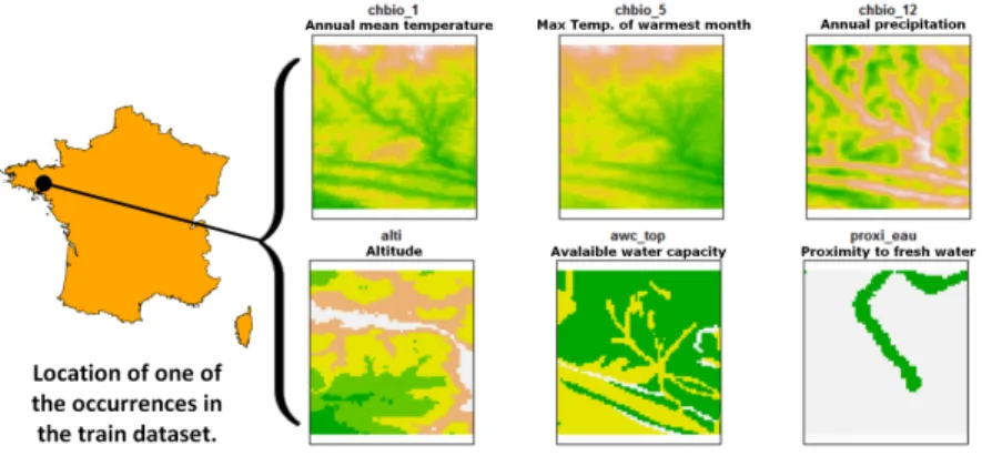
space, typically a feature vector composed of climatic variables (average temper-ature at that location, precipitation, etc.) and other variables such as soil type, land cover, distance to water, etc. The originality of GeoLifeCLEF is to gener-alize such niche modeling approach to the use of an image-based environmental representation space. Instead of learning a model from environmental feature vectors, participants may learn a model from k-dimensional image patches, each patch representing the value of an environmental variable in the neighborhood of the occurrence (see Figure 1 below for an illustration). From a machine learn-ing point of view, the challenge will thus be treatable as a multi-channel image classification task.
Fig. 1. Example of 6 channels from the environmental tensor of an occurrence. Each channel is an environmental heatmap, i.e. a matrix representing the values of an envi-ronmental variable in a square spatial area centered at the occurrence location.
2
Dataset
The participants were provided with a train and test set of species geolocated occurrences. Both were first composed of a .csv file with the occurrences spatial coordinates, the punctual values of environmental variables at the occurrence location, and, for the train table, the species name and identifier. Secondly, each row of the table (train and test) referred to a 33-channel image containing the environmental tensor extracted at that location.
2.1 Species occurrences
Occurrences data were extracted from the Global Biodiversity Information Facil-ity platform (GBIF6). To achieve precise species prediction from a geolocation,
the geolocations in question must be as precise as possible. However, a high number of occurrences from the GBIF have a spatially degraded geolocation for conservation reasons. Thus, we have chosen source datasets with undegraded geolocations in France, which are :
1. Carnet en ligne from Tela Botanica.
2. Cartographie des Leguminosae (Fabaceae) en France from Tela Botanica. 3. Naturgucker dataset.
4. iNaturalist Research-grade Observations.
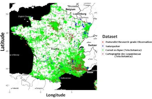
Only observations falling in the metropolitan French territory were kept so as to focus on a region for which we had an easy access to rich and homogeneous environmental descriptors for the whole dataset. Occurrences with uncertain names, as notified by the GBIF, were removed. The full dataset is finally com-posed of 291,392 occurrences. The labels to be predicted within the challenge are the species identifier (field species glc id). There are 3,336 species identifiers in total, and their associated taxonomic names are provided by the field es-pece retenue bdtfx (bdtfx referential 4.1). Due to some unreferenced hetero-geneity in the data collection protocol (naturalists checklists, conversion of site name to geolocation, etc), some geographical points accumulate several occur-rences. Indeed, there are in total 75,668 distinct geolocations (with a maximum of 527 points in one geolocation). All occurrences geolocations are represented in Figure 2. It reveals the bias in the spatial distribution of the occurrences.
2.2 Environmental data
Each occurrence is characterized by 33 local environmental images of 64x64 pix-els. These environmental images were constructed from various open datasets and include 19 bioclimatic quantitative variables at 1km resolution from Chelsea Climate [6], 10 pedological ordinal variables at 1km resolution from ESDB soil pedology data [11,12,16], one land cover categorical descriptor at 100 meters resolution from Corine Land Cover 2012 soil occupation data (version 18.5.1, 12/2016), one potential evapo-transpiration quantitative variable at 1km resolu-tion from CGIAR-CSI evapotranspiraresolu-tion data ([18,19]), one elevaresolu-tion quantita-tive variable at 90 meters resolution from USGS Elevation data (Data available from the U.S. Geological Survey and downloadable on the Earthexplorer7) and
one indicator of fresh water proximity at 12,5m resolution from the BD Carthage hydrologic data. As each of those variables are stored in large raster covering the French geographical territory. For any occurrence, we crop a 64 × 64 pixels window centered on the occurrence geolocation from the raster of each envi-ronmental variable. This way, we make the 64 × 64 × 33 envienvi-ronmental tensor
6
https://www.gbif.org/
7
Fig. 2. Occurrences geolocations in GeoLifeCLEF 2018 and their source dataset over the metropolitan territory.
associated with this occurrence. Besides, the punctual environmental values asso-ciated with an occurrence, are simply the extracted cell’s values from the rasters at the occurrence geolocation.
2.3 Train and test sets
The total of 291,392 occurrences were randomly split into a training set (218,543) and a test set (72,849) with the constraints that :
– For each species in the test set, there is at least one observation of it in the training set.
– An observation of a species in the test set is distant of more than 100 meters from all observations of this species in the train set to avoid major reporting dependencies.
Thus, the final train set contained all of the 3,336 species, while the test set contained 3,209 species.
3
Task Description
For every occurrence of the test set, participants must supply a list of 100 species maximum, ranked without ex-aequo. The used evaluation metric is the Mean
Reciprocal Rank (MRR). The MRR is a statistic measure for evaluating any process that produces a list of possible responses to a sample of queries ordered by probability of correctness. The reciprocal rank of a query response is the multiplicative inverse of the rank of the correct answer. The MRR is the average of the reciprocal ranks for the whole test set:
M RR = 1 Q Q X q=1 1 rankq
where Q is the total number of query occurrences xq in the test set and rankq
is the rank of the correct species y(xq) in the ranked list of species predicted by
the evaluated method for the occurrence xq.
4
Participants and methods
22 research groups registered to the GeoLifeCLEF challenge 2018. Among this large raw audience, 3 research groups finally succeeded in submitting run files. Details of the used methods and evaluated systems are synthesized below and further developed in the working notes of the participants ([2], [15] and [8]). Ta-ble 1 reports the results achieved by each run as well as a brief synthesis on the methods used in each of them. Complementary, the following paragraphs give a few more details about the methods and the overall strategy employed by each participant.
FLO team, France, 10 runs, [2]: FLO developed four prediction models, (i) one convolutional neural network trained on environmental tensors (FLO 3). The CNN implemented a customized architecture. It also treated the categori-cal land cover descriptor independantly from quantitative variables for the pri-mary layers. Activation’s of both variables types where then fused in deeper layers. (ii) one neural network (FLO 2) trained on species occurrences falling at the closest spatial point and two other models only based on the spatial occurrences of species: (iii) a closest-location classifier (FLO 1) and (iv) a ran-dom forest fitted on the spatial coordinates (FLO 4). Other runs correspond to late fusions of that base models, either by simply averaging either the output probabilities (FLO 5,FLO 6,FLO 7,FLO 8), or ranks with the Borda method (FLO 9,FLO 10).
ST team, Germany, 16 runs, [14]: ST experimented two main types of models, convolutional neural networks on environmental tensors with different data augmentations like rotation and flip of images (ST 1, ST 3, ST 11, ST 14, ST 15, ST 18, ST 19) and Boosted Trees (XGBoost) on vectors of environmental variables concatenated with spatial positions (ST 6, ST 9, ST 10, ST 12, ST 13, ST 16, ST 17). They also proposed a nearest-neighbor classifier based on the environmental variables of occurrences (ST 5), and two species cluster models
(ST 17,ST 8) where groups of species are constituted by the similarity of the environmental variables where they occur. For analysis purposes, ST 2 corre-sponds to a random predictor and ST 7 to a constant predictor returning always the 100 most frequent species (ranked by decreasing value of their frequency in the training set).
SSN, India, 4 runs, [10]: SSN attempted to learn a CNN-LSTM hybrid model, based on a ResNext architecture [17] extended with an LSTM layer [3] aimed at predicting the plant categories at 5 different levels of the taxonomy (class, then order, then family, then genus and finally species). The four runs are derived from this model.
5
Results
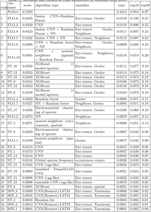
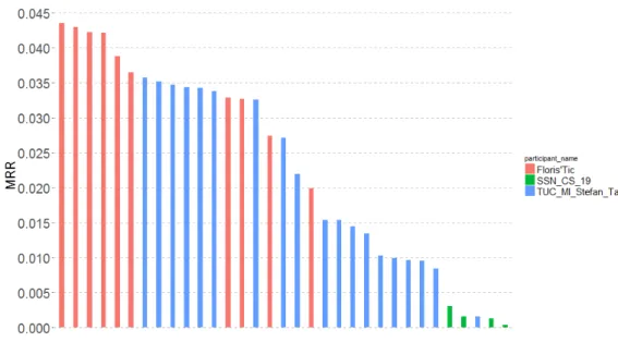
We report in Figure 3 and Table 1 the main results achieved by the 33 sub-mitted runs as well as some synthetic information about the used methods and variables for each run. The main conclusions we can draw from that results are the following:
Convolutional Neural Networks outperformed boosted trees: Boosted trees are known to provide state-of-the-art performance for environmental mod-elling. They are actually used in a wide variety of ecological studies [4,1,7,9]. Our evaluation, however, demonstrate that they can be consistently outper-formed by convolutional neural networks trained on environmental data tensors. The best submitted run that does not result from a fusion of different models (FLO 3), is actually a convolutional neural network trained on the environmen-tal patches. It achieved a M RR of 0.043 whereas the best boosted tree (ST 16) achieved a M RR of 0.035. As another evidence of the better performance of the CNN model, the six best runs of the challenge result from the combina-tion of it with the other models of the Floris’Tic team. Now, it is important to notice that the CNN models trained by the ST team (ST 1, ST 3, ST 11, ST 14, ST 15, ST 18, ST 19) and SSN team did not obtain good performance at all (often worse than the constant predictor based on the class prior distri-bution), which could be due to a mismatch of species identifiers, as noticed by the participant. For team ST, results can’t be interpreted directly as a failure of the methods. The ranking of runs in the test set was not consistent with validation results and the learning process can be improved according to [15]. This illustrates the difficulty of designing and fitting deep neural networks on new problems without former references in the literature. Lastly, the approaches trying to adapt existing complex CNN architectures that are popular in the image domain (such as VGG [13], DenseNet [5], ResNEXT [17] and LSTM [3]) were not successfull. High difference of performances in CNN learned with home-made architectures (F LO 6, F LO 3, F LO 8, F LO 5, F LO 9, F LO 10 compared to ST 3, ST 1) could underline the importance of architecture choices.
Purely spatial models are not so bad: the random forest model of the FLO team, fitted on spatial coordinates solely (FLO 4), achieved a fair M RR of 0.0329, close to the performance of the boosted trees of the ST team (that were trained on environmental & spatial data). Purely spatial models are usually not used for species distribution modelling because of the heterogeneity of the observations density across different regions. Indeed, the spatial distribution of the observed specimens is often more correlated with the geographic preferences of the observers than with the abundance of the observed species. However the goal of GeoLifeClef is to predict the most likely species to observe given the real presence of a plant. Thus, the heterogeneity of the sampling effort should induce less bias than in ecological studies.
It is likely that the Convolutional Neural Network already captured the spatial information: The best run of the whole challenge (FLO 6) results from the combination of the best environmental model (CNN FLO 3) and the best spatial model (Random forest FLO 4). However, it is noticeable that the improvement of the fused run compared to the CNN alone is extremely tight (+ 0.0005), and actually not statistically significant. In other words, it seems that the information learned by the spatial model was already captured by the CNN. Besides, CNN uses the whole environmental tensor as input and is better than the XGBoost methods which used only the average of each environmental matrix as input. So it is likely that CNN captured more information than the average of the environmental image. It might be some patterns associated with a particular area, or more generic environmental patterns (a wet valley, etc.). The learning of species communities patterns has potential: We first state that species have marked spatial patterns. Indeed, predicting the nearest species in space (FLO 1) or in the environmental space (ST 5) is much more efficient than simply listing species per global abundance (ST 7), which corre-sponds to a uniform prior on spatial distribution of each species. Second, meth-ods that allow interactions between species abundance, either by building and predicting group of species that have similar environmental preferences (ST 17), or learning the association between species that co-occur in a close surround-ing (FLO 2) perform better than simple nearest-neighbor approaches. However, these approaches are still limitating as, for example, FLO 2 only used the closest point as input information about surrounding species. Besides, even though the good performance of ST 17, there was very few groups of more than 1 species in their algorithm, which leaves small chances to predict non-common species while they represent the majority of species.
A significant margin of progress but still very promising results: even if the best MRR scores appear to be very low at a first glance, it is important to relativize them with regard to the nature of the task. Many species (tens to hundred) are actually living at the same location so that achieving very high MRR scores is not possible. The MRR score is useful to compare the methods between each others but it should not be interpreted as for a classical information retrieval task. In the test set itself, several species are often observed at exactly the same location. So that there is a max bound on the achievable MRR equal to
0.56. The best run (FLO 3) is still far from this max bound (MRR=0.043) but it is much better than the random or the prior distribution based MRR. Concretely, it retrieves the right species in the top-10 results in 25% of the cases, or in the top-100 in 49% of the cases (over 3, 336 species in the training set), which means that it is not so bad at predicting the set of species that might be observed at that location.
Table 1: Methods and results of runs submitted to GeoLifeCLEF2018.
rank
run-name score algorithm type variables top1 top10 top30
Perfect 0.5593 0.4214 0.854 0.97
1 FLO 6 0.0435 fusion: CNN+Random
Forest Env.tensor, Geoloc 0.0116 0.100 0.25
2 FLO 3 0.0430 CNN Env.tensor 0.0110 0.098 0.25
3 FLO 8 0.0423 fusion: CNN + Random Forest + NN
Env.tensor, Geoloc,
Neighbors 0.0111 0.097 0.24
4 FLO 5 0.0422 fusion: CNN + NN Env.tensor, Neighbors 0.0112 0.097 0.24 5 FLO 9 0.0388 CNN + Random forest
+ NN Env.tensor, Geoloc, Neighbors 0.0099 0.088 0.22 6 FLO 10 0.0365 CNN + nearest-neighbors (spatial) + Random Forest Env.tensor, Neighbors, Geoloc 0.0116 0.074 0.20 7 ST 16 0.0358 XGBoost (1
model/species) Env.tensor, Geoloc 0.0111 0.077 0.18
8 ST 13 0.0352 XGBoost Env.tensor, Geoloc 0.0114 0.075 0.18
9 ST 10 0.0348 XGBoost Env.tensor, Geoloc 0.0113 0.073 0.18
10 ST 9 0.0344 XGBoost Env.tensor, Geoloc 0.0108 0.073 0.18
11 ST 12 0.0343 XGBoost Env.tensor, Geoloc 0.0110 0.072 0.18
12 ST 6 0.0338 XGBoost (1
model/species) Env.tensor, Geoloc 0.0104 0.072 0.18
13 FLO 4 0.0329 Random forest Geoloc 0.0098 0.071 0.17
14 FLO 7 0.0327 NN + Random forest Neighbors, Geoloc 0.0093 0.071 0.18 15 ST 17 0.0326 Environmental
cluster-ing of species Env.tensor, Geoloc 0.0106 0.068 0.16
16 FLO 2 0.0274 NN Neighbors 0.0079 0.057 0.15
17 ST 5 0.0271 nearest-neighbors
(envi-ronment, spatial) Neighbors 0.0098 0.051 0.14
18 ST 8 0.0220 Environmental
cluster-ing of species Env.tensor, Geoloc 0.0087 0.043 0.08 19 FLO 1 0.0199 nearest-neighbors
(spa-tial) Geoloc 0.0077 0.042 0.09
20 ST 3 0.0153 CNN Env.tensor 0.0047 0.029 0.08
21 ST 1 0.0153 CNN Env.tensor 0.0047 0.029 0.08
22 ST 14 0.0144 CNN Env.tensor 0.0040 0.030 0.07
23 ST 7 0.0134 Global species frequency occurrences counts 0.0026 0.033 0.08
24 ST 15 0.0103 CNN (vgg-like) Env.tensor 0.0046 0.019 0.03
25 ST 19 0.0099 standard DenseNet121
CNN Env.tensor 0.0021 0.024 0.05
26 ST 11 0.0096 CNN (vgg-like) Env.tensor 0.0022 0.022 0.05
27 ST 18 0.0096 ensemble CNN (vgg-like) Env.tensor 0.0019 0.023 0.05
28 ST 4 0.0085 XGBoost Env.tensor, spatial 0.0021 0.022 0.04
29 SSN 3 0.0030 CNN(Resnext)-LSTM Env.tensor, Taxonomy 0.0006 0.006 0.02 30 SSN 4 0.0016 CNN(Resnext)-LSTM Env.tensor, Taxonomy 0.0000 0.005 0.01
31 ST 2 0.0016 Random list 0.0003 0.003 0.01
32 SSN 2 0.0013 CNN(Resnext)-LSTM Env.tensor, Taxonomy 0.0001 0.002 0.01 33 SSN 1 0.0004 CNN(Resnext)-LSTM Env.tensor, Taxonomy 0.0001 0.002 0.00
Fig. 3. MRR scores per submitted run and participant.
6
Complementary Analysis
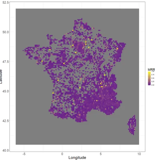
Spatial heterogeneity of model performances: We computed the MRR restricted to occurrences that fall in spatial quadrats of 10×10 km all over the French territory. We projected this on a map in Figure 4. The global perfor-mances of the methods hide spatial heterogeneity, as shown in the map. Indeed, Paris is the best predicted area, then the Mediterranean region and the Alpes. Then other regions like the Loire, the Pyrenees and the Atlantic coastline. One could think this is due to the larger number of points available in these areas, but this is not exactly true. Complementary analysis showed that the impor-tantly sampled areas had a more stable MRR but not higher in average. Thus, improving models predictions should pass by finding reasons of varying regional performances, in the hope to bring a solution.
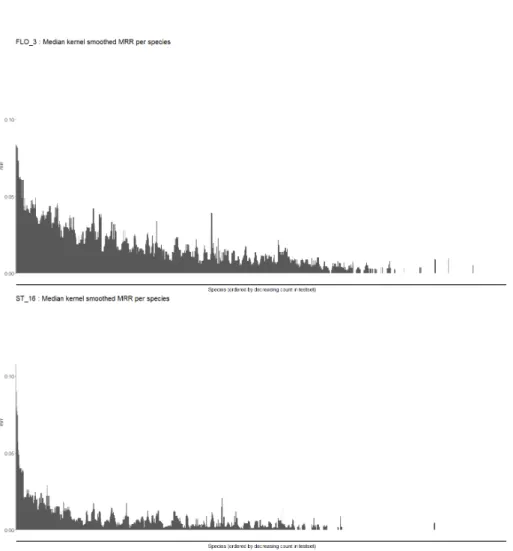
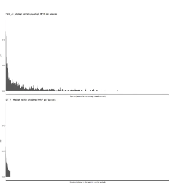
Rare species are not unpredictable: For each species and method, we calculated the MRR over the occurrences of this species in the test set. We ordered species per decreasing global occurrences count in the test set in order to compare the performances of each method along the gradient from common to rare species. The raw graphs were difficult to analyse because the MRR varies
importantly for rare species, as there are very few occurrences. Thus, we operate a smoothing along the scarcity gradient. For each species we took the median of the MRR over the 40 species of closest rank on this scarcity gradient. Figures 5 and 6 show the result for FLO 3 (environmental CNN), ST 16 (XGBoost), FLO 4 (spatial Random Forest) and ST 7 (Global frequency of species). One can see that ST 7 early cancels along the scarcity gradient. This is because more than 50% of the species over which the median is calculated have a null MRR, which correctly represents the tendancy we want to observe. First, it seems that non-common species have marked spatial preferences because FLO 4 is much better when getting scarcer than ST 7. Second, the progression of predictions of FLO 3 and ST 16 compared to FLO 4 for rare species (in the long tail) suggests that those species mainly have marked environmental preferences that is not easy to capture with a spatial model which doesn’t have access to this information. The CNN is very good at predicting non-common species, which may be a bit surprising as (i) its predictions should be smooth in space according to the width of some environmental images (64x64km for climatic and pedological variables) and the chosen architecture and (ii) rare species often have a restricted niche.
7
Conclusion
We have analyzed the results of the 3 participants of GeoLifeCLEF 2018. CNN models learnt on environmental tensors revealed to be the most performing method, however challenging to operate. According to those results, they are more efficient than Boosted Trees a state of the art method in species distri-bution modeling. This might be because they may detect particular area or environmental patterns as they access to the full surrounding environment data, but that remain to be proved. Spatial and species association methods have shown reasonably good results, but there is room for improvement, especially for the use of interdependence. The complementary analysis revealed that all methods had the same areas of unreliability. Furthermore, the integration of environmental variables seems to be very beneficial to the prediction of non-common species. The task of finding the species found at a precise location is difficult because many species co-exist at very small spatial scales (under the meter). The accuracy of current geolocation devices doesn’t even allow to indi-cate with this precision the point where the specimen was observed. Thus, in the future, the evaluation process shouldn’t penalize predictions of other species that have been observed in such a close surrounding regarding the precision of the reported geolocation.
Fig. 5. Smoothed MRR per species for FLO 3 and ST 16. Species are ordered by number of occurrences in the test set. Each species MRR is smoothed by taking the median over the MRR the 40 species of closest rank along the scarcity gradient.
Fig. 6. Smoothed MRR per species for FLO 4 and ST 7. Species are ordered by number of occurrences in the test set. Each species MRR is smoothed by taking the median over the MRR the 40 species of closest rank along the scarcity gradient.
References
1. De’Ath, G.: Boosted trees for ecological modeling and prediction. Ecology 88(1), 243–251 (2007)
2. Deneu, B., Servajean, M., Botella, C., Joly, A.: Location-based species recommen-dation using co-occurrences and environment - geolifeclef 2018 challenge. In: CLEF working notes 2018 (2018)
3. Gers, F.A., Schmidhuber, J., Cummins, F.: Learning to forget: Continual prediction with lstm (1999)
4. Guisan, A., Thuiller, W., Zimmermann, N.E.: Habitat Suitability and Distribution Models: With Applications in R. Cambridge University Press (2017)
5. Huang, G., Liu, Z., Weinberger, K.Q., van der Maaten, L.: Densely connected convolutional networks. In: Proceedings of the IEEE conference on computer vision and pattern recognition. vol. 1, p. 3 (2017)
6. Karger, D.N., Conrad, O., B¨ohner, J., Kawohl, T., Kreft, H., Soria-Auza, R.W., Zimmermann, N., Linder, H.P., Kessler, M.: Climatologies at high resolution for the earth’s land surface areas. arXiv preprint arXiv:1607.00217 (2016)
7. Messina, J.P., Kraemer, M.U., Brady, O.J., Pigott, D.M., Shearer, F.M., Weiss, D.J., Golding, N., Ruktanonchai, C.W., Gething, P.W., Cohn, E., et al.: Mapping global environmental suitability for zika virus. Elife 5 (2016)
8. Moudhgalya, N.B., Sundar, S., Divi, S., Mirunalini, P., Aravindan Bose, C.: Hierar-chically embedded taxonomy with clnn to predict species based on spatial features. In: CLEF working notes 2018 (2018)
9. Moyes, C.L., Shearer, F.M., Huang, Z., Wiebe, A., Gibson, H.S., Nijman, V., Mohd-Azlan, J., Brodie, J.F., Malaivijitnond, S., Linkie, M., et al.: Predicting the geo-graphical distributions of the macaque hosts and mosquito vectors of plasmodium knowlesi malaria in forested and non-forested areas. Parasites & vectors 9(1), 242 (2016)
10. Nithish B Moudhgalya, Sharan Sundar, S.D.M.P., Bose, C.A.: Hierarchically em-bedded taxonomy with clnn to predict species based on spatial features. In: CLEF working notes 2018 (2018)
11. Panagos, P.: The european soil database. GEO: connexion 5(7), 32–33 (2006) 12. Panagos, P., Van Liedekerke, M., Jones, A., Montanarella, L.: European soil data
centre: Response to european policy support and public data requirements. Land Use Policy 29(2), 329–338 (2012)
13. Simonyan, K., Zisserman, A.: Very deep convolutional networks for large-scale image recognition. CoRR abs/1409.1556 (2014)
14. Stefan Taubert, Max Mauermann, S.K.D.K., Eibl, M.: Species prediction based on environmental variables using machine learning techniques. In: CLEF working notes 2018 (2018)
15. Taubert, S., Mauermann, M., Kahl, S., Kowerko, D., Eibl, M.: Species prediction based on environmental variables using machine learning techniques. In: CLEF working notes 2018 (2018)
16. Van Liedekerke, M., Jones, A., Panagos, P.: Esdbv2 raster library-a set of rasters derived from the european soil database distribution v2. 0. European Commission and the European Soil Bureau Network, CDROM, EUR 19945 (2006)
17. Xie, S., Girshick, R., Doll´ar, P., Tu, Z., He, K.: Aggregated residual transformations for deep neural networks. In: Computer Vision and Pattern Recognition (CVPR), 2017 IEEE Conference on. pp. 5987–5995. IEEE (2017)
18. Zomer, R.J., Bossio, D.A., Trabucco, A., Yuanjie, L., Gupta, D.C., Singh, V.P.: Trees and water: smallholder agroforestry on irrigated lands in Northern India, vol. 122. IWMI (2007)
19. Zomer, R.J., Trabucco, A., Bossio, D.A., Verchot, L.V.: Climate change mitigation: A spatial analysis of global land suitability for clean development mechanism af-forestation and reaf-forestation. Agriculture, ecosystems & environment 126(1), 67–80 (2008)