HAL Id: halshs-00460472
https://halshs.archives-ouvertes.fr/halshs-00460472
Submitted on 3 Mar 2010
HAL is a multi-disciplinary open access archive for the deposit and dissemination of sci-entific research documents, whether they are pub-lished or not. The documents may come from teaching and research institutions in France or
L’archive ouverte pluridisciplinaire HAL, est destinée au dépôt et à la diffusion de documents scientifiques de niveau recherche, publiés ou non, émanant des établissements d’enseignement et de recherche français ou étrangers, des laboratoires
A Short Note on the Nowcasting and the Forecasting of
Euro-area GDP Using Non-Parametric Techniques
Dominique Guegan, Patrick Rakotomarolahy
To cite this version:
Dominique Guegan, Patrick Rakotomarolahy. A Short Note on the Nowcasting and the Forecasting of Euro-area GDP Using Non-Parametric Techniques. Economics Bulletin, Economics Bulletin, 2010, 30 (1), pp.508-518. �halshs-00460472�
A Short Note on the Nowcasting and the Forecasting of
Euro-area GDP Using Non-Parametric Techniques
Dominique Guégan∗, Patrick Rakotomarolahy† December 30, 2009
Abstract
The aim of this paper is to introduce a new methodology to forecast the monthly economic indicators used in the Gross Domestic Product (GDP) modelling in order to improve the forecasting accuracy. Our approach is based on multivariate k-nearest neighbors method and radial basis function method for which we provide new theoretical results. We apply these two methods to compute the quarter GDP on the Euro-zone, comparing our approach, with GDP obtained when we estimate the monthly indicators with a linear model, which is often used as a benchmark.
.
Keywords: k-nearest neighbors method - radial basis function method - non-parametric forecasts - GDP - Euro-area.
∗Paris School of Economics, CES-MSE, Université Paris 1 Panthéon-Sorbonne, 106 boulevard de l’Hopital
75647 Paris Cedex 13, France, e-mail: [email protected]
†CES-MSE, Université Paris 1 Panthéon-Sorbonne, 106 boulevard de l’Hopital 75647 Paris Cedex 13, France,
1
Introduction
The aim of this paper is to introduce a new methodology to forecast the monthly economic indi-cators used in the Gross Domestic Product (GDP) modelling in order to improve the forecasting accuracy.
The GDP is only available on quartely basis with a time span of 2 or 3 months, and sometimes with significant revisions. Thus, governments and central banks need to have accurate tools to update consistently the information used to revise and provide good forecasts for GDP. In short term economic, monthly indicators are routinely used to assess the current economic conditions before GDP figures are made available. There exists different ways to use these monthly indicators in order to provide a forecast of the quartely GDP. They appear, for instance, in dynamic factor models Kapetanios and Marcellino (2006), MIDAS regressions, Marcellino and Schumacher (2008), structural models, Clements and Hendry, (1999) or bridge equations, Baffigi et al. (2004) or Darne (2008). In all cases, the estimation of the monthly indicators is determinant.
In this paper we focus on a new approach providing accurate forecasts of the monthly indicators that we plug in bridge equations to obtain the Euro-area GDP. We use 13 macro-economic indicators and the eight equations proposed by Diron (2008). Our methodology is based on non-parametric techniques. The non-parametric techniques that we use in this paper work in a multivariate setting: they are the multivariare nearest neighbors (NN) method and the radial basis function (RBF) method. Assuming that we observe an economic indicator X, on a given period, say X1,· · · , Xn, we embed this information set in a space of dimension d∈ N∗ to build
NN or RBF forecasts ˆXn+h, h≥ 1 , that we use in fine in the GDP equations. We provide the
algorithm that we use for both methods and also the theoretical results proving the accuracy of the forecasts under very smooth assumptions. We apply these methods to compute the quarter GDP on the Euro-zone, comparing our approach, with GDP obtained when we estimate the monthly indicators with a linear model, which is often used as a benchmark.
We describe in Section two our methodology providing also consistent results. In section three, we exhibit the nowcasting and forecasting of the GDP.
2
The methodology
We describe two methods we consider here, the multivariate NN and RBF methods, Yatchew (1998) and references therein. The problem that we face consists to estimate a regression function
m(.) linking two random variables Y = m(X). This estimate will have the following representa-tion, mn(x) =Pni=1ωi,n(x)Yi, where ωi,n are weights to be specified, Silverman (1986), Guégan
(2003).
Assuming that we observe a time series in R, we transform the original data set embedding it in a space of dimension d, building vectors (Xn)n⊂ Rd. The embedding is interesting because
it permits different features of the data to be taken into account which are not observed on the trajectory. We are interested to get an estimate of m(x), x∈ Rd, using the k closest vectors of
Xninside the training set S ⊂ Rdif we work with the NN method, and if we work with the RBF
approach, we want to estimate m(.) by a set of k clusters through a radial basis functions φ. We detail now the methodology to estimate m(.).
1. Multivariate k-NN estimate for m(.). After embedding, we determine the k closest vectors of Xn= (Xn−d+1,· · · , Xn) inside the training set S⊂ Rd :
S ={Xℓ+d = (Xℓ+1,· · · , Xℓ+d)| l = 0, ..., ℓ = n − d − 1}.
Denoting by X(i) i= 1, ..., k(n), the ith nearest neighbor of x, then mn(x) =
X
X(i)∈S,i∈N (x)
w(x− X(i))X(i)+1, (2.1) is the k-NN estimate of m(x). A general form for the weights is:
w(x− X(i)) = 1 nRd nK( x−X(i) Rn ) 1 nRd n Pn i=1K( x−X(i) Rn ) ,
where K(.) is a given weighting function vanishing outside the unit sphere in Rd and R n
is the distance between the kth NN of x and x itself. In this multivariate NN method, we need to detect the neigbors, and to choose the weights. In practice, one often restricts to exponential weight, K(x−X(i)
Rn ) = exp(−||x−X(i)||
2) or to uniform weight, K(x−X
(i)) = k1.
2. RBF estimate for m(.). As soon as the data have been embedded in a space of dimension d, we create (n− d + 1) vectors. Then, we use a k-means method to partition these vectors providing k clusters, denoted by Ci, i = 1, ..., k. Each vector belongs to the cluster such
that its distance to the cluster’s center is minimal, then, mn(x) = w0+
k
X
i=1
is the RBF estimate of m(x). The parameters ci = (ci1, ..., cid)∈ Rd, ri ∈ R and wi ∈ R have
to be estimated. The radial basis function φ(.) can be chosen among Gaussian, multiquadric or inverse multiquadric functions, Guégan (2003) for examples. As soon as the function φ and the parameters (ci, ri), i = 1, ..., k are known, then φ(kx − cik , ri) is known and the
function m(x) is linear in wi thus wi is estimated by ordinary least squares method.
For both methods, all the parameters are determined in a space of dimension d. The properties of these estimates are given in the theorem below which provides new results. We now specify the assumptions needed to establish these properties.
We assume that we observe a strictly stationary time series (Xn)n that is characterized by an
invariant measure with density f , the random variable Xn+1 | (Xn = x) has a conditional
density f (y | x), and the invariant measure associated to the embedded time series {Xn =
(Xn−d+1,· · · , Xn)} is h. On the other hand:
H0: The time series (Xn)nis φ-mixing.
H1: m(x), f (y| x) and h(x) are p continuously differentiable functions.
H2: The function f (y| x) is bounded,
H3: There exists a sequence k(n) < n such thatPk(n)i=1 wi → 1 as n→ ∞.
H4: For k-NN method, if w(x) = k(n)1 , then σ2 = V ar(Xn+1 | Xn = x); if w(x)∈ R depending
(or not) on (Xn)n, then σ2= γ2(V ar(Xn+1| Xn= x)), where γ∈ R+.
H5: For RBF mehtod, φ is Gaussian and the estimated weights wi in (2.2) satisfy (wi− ci d+1 A )→ 0 as n→ ∞, where ci d+1 = N1i P j,Xj∈CiXj+1, Ni = #Ci and A = Pk j=1exp(− kx−cjk2 2r2 j ).
Theorem 2.1. We assume that {Xn} is a stationary time series and that the assumptions H0 -H2 are verified. Moreover, for the multivariate NN estimate (2.1), we asume that H3-H4 are
verified, and for the RBF estimate (2.2) we assume that H5 is verified, then :
√ nQ(m
n(x)− Emn(x))→DN (0, σ2), (2.3)
with 0≤ Q < 1, and Q = 2p+d2p .
Proof: In case of multivariate NN approach, the convergence has been proven in Guégan and Rakotomarolahi (2009). In case of the RBF estimate, we can prove the same result remarking that φ(y, r) = exp(−2ry22) and wi =
ci d+1 A with A = Pk j=1exp(− kx−cjk2 2r2 j
for multiquadric radial basis function using the approximation √ 1 y2+r2 = exp(− 1 2log(y2+ r2))≈ 1 rexp(− y2
2r2), when the centers ci are close to x.
This theorem provides results on robust estimation of regression, justifying the use of nonpara-metric methods to construct estimates from dependent variables. It extends the known results in the independent case for k-NN estimate to dependent variables, Stute (1984) and Yakowitz (1987). It provides new results for RBF estimation. Thanks to the asymptotic normality, it is also possible to exhibit confidence intervals, Guégan and Rakotomarolahy (2009), and to build density forecasts which can be used as back testing procedure.
3
Carrying out of the method
Information on the current state of economic activity is a crucial ingredient for policy making. Economic policy makers, international organisations and private sector forecasters commonly use short term forecasts of real gross domestic product (GDP) growth based on monthly indicators. For users, an assessment of the reliability of these tools, and of the source of potential forecast errors is essential. In the exercise that we present below, we wish to show that beyond the model chosen to calculate the GDP in the end, the forecasts of monthly economic indicators used in the final model are fundamental and may be misleading not negligible if they are not properly estimated.
We therefore consider the approach of bridge equations to calculate the GDP in the final stage, limiting ourselves to the 8 equations introduced in the paper of Diron (2008), each equation providing a model of GDP, denoted Yi
t, i= 1,· · · , 8. They are finally aggregated consistently to
provide a final value of GDP, denoted Yt. Each equation is calculated from monthly economic
indicators, 13 in total denoted Xi
t, i= 1,· · · , 13, they are listed in table 1. To realize this
objec-tive, we use the real-time data base provided by EABCN through their web site1.
The real-time information set starts in January 1990 when possible (exceptions are the confidence indicator in services, that starts in 1995, and EuroCoin, that starts in 1999) and ends in November 2007. The vintage series for the OECD composite leading indicator are available through the
OECD real-time data base 2. The EuroCoin index is taken as released by the Bank of Italy.
The vintage data base for a given month takes the form of an unbalanced data set at the end of the sample. To solve this issue, we apply the non-parametric methodology to forecast the monthly variables in order to complete the values until the end of the current quarter for GDP nowcasts and until the end of the next quarter for GDP forecasts, then we aggregate the monthly data to quarterly frequencies. We use four various ways to forecast the monthly variables: an ARIMA(p,d,0) approach, the k-NN procedure (d = 1 and d > 1) with exponential weights and the radial basis function method with various couples (d, k), and various functions φ(·, ·). We present now the four procedures. For the three first methods the economic indicators have been made stationary in presence of trend.
1. Concerning the ARIMA(p,d,0) procedure, for each economic indicator we use the Akaike criterion AIC for the selection of the lag p. Model’s parameters are estimated by least square method.
2. Regarding the NN method when d = 1, we determine the number of neighbors k by min-imizing : qn−k1 Pn
t=k|| ˆXt+1i − Xt+1i ||2, i = 1,· · · , 13, where n is the sample size, ˆXt+1i is
the estimate of the i-th economic indicator Xi
t+1 obtained from (2.1) with d = 1. When the
number k is determined for the horizon h = 1, we used it to calculate the forecasts for h > 1. This work is done for each economic indicator, and therefore the number of neighbors k may not be the same for all indicators.
3. The multivariate k-NN method: (i) we embed the initial serie X1, ..., Xn in a space of
di-mension d building vectors {Xd, Xd+1, ..., Xn} in Rd, where Xi = (Xi−d+1, ..., Xi)}; (ii) we
determine the k nearest vectors of Xninside these vectors, and denote ri =kXn− Xik, i =
d, d+1, ..., n−1, the distance between these vectors. We order the sequence rd, rd+1, ..., rn−1
such that r(d) < r(d+1) < ... < r(n−1), and we detect the vectors X(j) corresponding to r(j), j = d, d + 1, ..., d + k − 1; (iii) to compute mn(Xn) = ˆXn+1, we use the
ex-pression (2.1). It may be noted that we obtain the one step ahead forecast. Finally we use the information set: X1, ..., Xn, ˆXn+1 instead of X1, ..., Xn and redo step (i)-(iii), to
get the two steps ahead forecast, and so on. We keep the couple (d, k) which minimizes q
1 n−k−d
Pn
t=k+d|| ˆXt+1i − Xt+1i ||2 for each indicator.
4. The RBF method: given a d-dimensional space, (i) we determine k clusters using a k-means clustering: this method permits to determine the centers and the radii (ci, ri),
i = 1, ..., k characterizing the clusters; (ii) for a given function φ, the vectors in Rd are
then grouped inside the k clusters. We estimate the width ri using the r centers cj (r≤ k)
which are closest to ci, such that, for i = 1, ..., k, ri = 1r
q Pr
j=1kci− cjk2 and finally the
weights wi are estimated by ordinary least squares method; (iii) the one-step-ahead value
obtained with the RBF method is given by the relationship (2.2); (iv) It is well known that k-means clustering provides local minimum, thus, we repeat this algorithm many times keeping parameters wich minimize the sumPn
j=d(Xj+1− m(Xj))2. Then, we consider the
information set: X1, ..., Xn, ˆXn+1 instead of X1, ..., Xnand redo step (i)-(iv) to get the two
steps ahead forecast, and so on. Using this RBF method do not need to make the series stationary, which constitutes a great advantage of the method in comparison with the three other ones. Here, the parameter d vary between 2 and 5, and k between 3 and 7, and can be different for each economic indicator.
As soon as the four modellings are retained, we compute the GDP flash estimates that were released in real-time by Eurostat from the first quarter of 2003 to the third quarter of 2007 using the previous forecasts of the monthly indicators. According to this scheme, the monthly series have to be forecast for an horizon h varying between 3 and 6 months in order to complete the data set at the end of the sample. Recall that the h-step-ahead predictor for h > 1 is estimated recursively starting from the one-step-ahead formula.
Using five years of vintage data, from the first quarter 2003 to the third quarter 2007, we provide RMSEs for the Euro area flash estimates of GDP growth in genuine real-time conditions. We have computed the RMSEs for the quarterly GDP flash estimates, obtained with the four forecasting methods used to complete adequately in real-time the monthly indicators, that is ARIMA, k-NN (d = 1 and d > 1) and RBF methods. More precisely, we provide the RMSEs of the combined forecasts based on the arithmetic mean of the eight equations of Diron (2008). Thus, for a given forecast horizon h, we compute ˆYtj(h) which is the predictor stemming from Diron’s equation j = 1,· · · , 8, in which we have plugged the forecasts of the monthly economic indicators, and we compute the final estimate GDP at horizon h: ˆYt(h) = 18P8j=1Yˆtj(h). the RMSE criterion
for the final GDP is RM SE(h) = q
1 T
PT
between Q1 2003 and Q4 2007 (in our exercise, T = 19) and Yt is the Euro area flash estimate
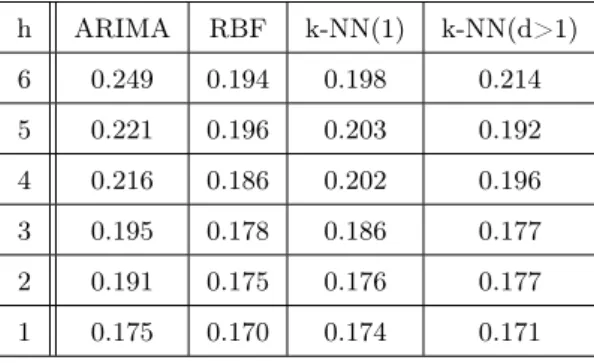
for quarter t. The RMSE errors for final GDP are provided in table 2 and comments follow.
The accuracy of the nowcating and forecasting increases as soon as the information set grows. Indeed, for all the four methods, if the forecast horizon reduces from h = 6 to h = 1, the RMSEs becomes lower. Few days before the publication of the flash estimate (around 13 days with h= 1), the lowest RMSE is obtained with the RBF method (RMSE=0.170). For all horizons h from 6 to 1, we can see that we have smaller RMSE using non parametric methods (RBF and k-NN) than using linear modelling. Moreover, with the nonparametric procedures, we obtain smaller error if we work in multivariate setting than in univariate approach. Concerning RBF and k-NN methods in multivariate setting, the k-NN method provides lower RMSE for h = 3, 5 , and for h = 1, 2, 4, 6 we get better results using RBF method: thus these two approaches appear competitive to predict the GDP Euro area. Finally, they give always smallest error than the methods developed in the univariate setting. This last result confirms the importance to work in a multivariate framework for GDP computing. Such remark has already been done by authors using factor models, Kapetanios and Marcellino (2006). The next step will be to compare both multivariate settings: parametric and non-parametric modellings, although there exists a big difference between these two modellings due to the fact that factor models typically use a large number of factors to be efficient, which is not the case here. Nevertheless this work has to be done and will be the purpose of a companion paper.
References
Baffigi A., Golinelli R. and Parigi G. (2004). Bridge model to forecast the euro area GDP. International Journal of Forecasting, 20, 447-460.
Clements, M. P., Hendry, D. F. (1999). Forecasting non-stationary economic time series. Cam-bridge: MIT Press.
Darne O. (2008) Using business survey in industrial and services sector to nowcast GDP growth:The French case, Economics Bulletin, 3(32), 1-8
Diron M. (2008) Short-term forecasts of Euro area real GDP growth: an assessment of real-time performance based on vintage data, Journal of Forecasting, Vol. 27, Issue 5, pp. 371-390. Guégan D. 2003. Les Chaos en Finance: Approche Statistique. Economica Série Statistique Mathématique et Probabilité: Paris.
Guégan D., Rakotomarolahy P. (2009) The Multivariate k-Nearest Neighbor Model for Depen-dent Variables: One-Sided Estimation and Forecasting, WP-2009, Publications du CES Paris 1 Panthéon-Sorbonne.
Kapetanios G., M. Marcellino (2006), A parametric estimation method for dynamic factors models of large dimensions, IGIER WP No 305, Bocconi University, Italy.
Marcellino M, Schumacher C. Factor-MIDAS for now and forecasting with ragged-edge data: A model comparison for German GDP. CEPR WP 2008: No 6708.
Stute W. 1984. Asymptotic normality of nearest neighbor regression function estimates. Annals
of Statistics 12 : 917-926.
Silverman BW. 1986. Density Estimation for Statistics and Data Analysis. Chapmann and Hall: London.
Yakowitz S. 1987. Nearest neighbors method for time series analysis. Journal of Time Series
Analysis 8 : 235-247.
Yatchew, A.J. (1998). Nonparametric regression techniques in economics. Journal of Economic
We provide the list of the monthly economic indicators used in this study for the computation of the GDP using the bridge equations.
Short Notation Notation Indicator Names Sources Period I1 IPI Industrial Production Index Eurostat 1990-2007 I2 CTRP Industrial Production Index in Eurostat 1990-2007
Construction
I3 SER-CONF Confidence Indicator in Services European Commission 1995-2007
I4 RS Retail sales Eurostat 1990-2007
I5 CARS New passenger registrations Eurostat 1990-2007 I6 MAN-CONF Confidence Indicator in Industry European Commission 1990-2007 I7 ESI European economic sentiment index European Commission 1990-2007 I8 CONS-CONF Consumers Confidence Indicator European Commission 1990-2007 I9 RT-CONF Confidence Indicator in retail trade European Commission 1990-2007 I10 EER Effective exchange rate Banque de France 1990-2007 I11 PIR Deflated EuroStock Index Eurostat 1990-2007 I12 OECD-CLI OECD Composite Leading Indicator, OECD 1990-2007
trend restored
I13 EUROCOIN EuroCoin indicator Bank of Italy 1999-2007
Table 1: Summary of the thirteen economic indicators of Euro area used in the eight GDP bridge equations. h ARIMA RBF k-NN(1) k-NN(d>1) 6 0.249 0.194 0.198 0.214 5 0.221 0.196 0.203 0.192 4 0.216 0.186 0.202 0.196 3 0.195 0.178 0.186 0.177 2 0.191 0.175 0.176 0.177 1 0.175 0.170 0.174 0.171
Table 2: RMSE for the estimated mean quarterly GDP, using AR, k-NN (d = 1 and d > 1), and RBF predictions for the monthly indicators.
![[PDF] Interface graphique java : combos sliders et spinners | Cours java](data:image/gif;base64,R0lGODlhAQABAIAAAP///wAAACH5BAEAAAAALAAAAAABAAEAAAICRAEAOw==)