HAL Id: hal-03045804
https://hal.archives-ouvertes.fr/hal-03045804
Submitted on 8 Dec 2020
HAL is a multi-disciplinary open access
archive for the deposit and dissemination of sci-entific research documents, whether they are pub-lished or not. The documents may come from
L’archive ouverte pluridisciplinaire HAL, est destinée au dépôt et à la diffusion de documents scientifiques de niveau recherche, publiés ou non, émanant des établissements d’enseignement et de
The Impact of Low-Carbon Policy on Stock Returns
Rania Hentati-Kaffel, Alessandro Ravina
To cite this version:
Rania Hentati-Kaffel, Alessandro Ravina. The Impact of Low-Carbon Policy on Stock Returns. SSRN Electronic Journal, 2020, �10.2139/ssrn.3444168�. �hal-03045804�
The impact of low-carbon policy on stock returns
Alessandro Ravinaa, Rania Hentati-Kaffelb
a,b Universit´e Paris I Panth´eon-Sorbonne, 106-112 Boulevard de l’Hˆopital, Paris, France
ARTICLE HISTORY Compiled February 10, 2020
ABSTRACT
This paper assesses the impact of low-carbon policy on stock returns by means of an environmental extension of Fama and French’s (2015) five factor model. This paper makes four major contributions. Firstly, for the first time a factor, GMC (green minus carbon), meant to provide the premium which results from not paying a carbon price is constructed. The GMC factor is obtained by means of a sample of 182 firms from 19 European countries operating in 35 sectors: from January 2008 to December 2018 the value-weight returns of 91 firms regulated by the 2003/87/CE directive are subtracted from the value-weight returns of 91 firms exempted by the 2003/87/CE directive upon which the EU-ETS is based. Secondly, we provide evidence that the addition of the GMC factor improves the performance of the 5 factor model in Europe in the 2008-2018 time span. Thirdly, results show that there is a high green premium rather than a carbon premium as it was asserted by parts of the literature, and that this green premium is highly statistically significant. Fourthly, after performing a carbon stress test, we show the effects of EU-ETS average price shocks on both carbon and green firms for each market cap tranche.
KEYWORDS
Low-carbon transition risks, EU-ETS, CO2emissions, asset pricing model, green
premium
1. Introduction
Climate change risks can be partitioned in two components: the risk associated with
the impacts of global warming on natural and human systems and the risk
origi-nating from anthropogenic climate change mitigation. Literature designates the first
component with the label “climate risk” (Carney, 2015): changes in extreme climate
phenomena — e.g. temperature extremes, high sea levels extremes, precipitation
ex-tremes (Intergovernmental Panel on Climate Change, 2014) —, are likely to cause
serious damages to agriculture, coastal zones, human health, and affect growth (Dell,
Jones, & Olken, 2014; Pycroft, Abrell, & Ciscar, 2016), productivity (Graff Zivin &
Neidell, 2014; Hallegatte, Fay, Bangalore, Kane, & Bonzanigo, 2015), the value of
finan-cial assets and insurance claims. Addressing climate change implies greenhouse gases
(GHG) mitigation: the process of adjustment towards a lower carbon economy carries
a cost that the literature refers to as “transition risk” or “carbon risk” (Caldecott &
McDaniels, 2014).
Low-carbon transition risk is a multi-faceted concept. It includes all drivers of risk
linked to the decarbonisation of the economy: pollution reducing market-based
instru-ments (a carbon price: a carbon tax, an auction price, or a secondary market price);
command and control induced technological shifts aimed at a reduction of CO2
emis-sions, e.g. stranded assets or assets that have suffered from unanticipated or premature
write-downs, devaluations, or conversion to liabilities (Caldecott et al., 2016); and
mar-ket risk, i.e. marmar-ket demands for low carbon products (Zhou et al., 2016). Marmar-ket based
instruments and command and control regulation find their genesis in low-carbon
pol-icy. The objective of this paper is to study the impact of low-carbon policy upon the
value of financial assets, particularly stock returns. Specifically, we seek to understand
and explain the impact of one particular European policy, the 2003/87/CE directive
upon which the EU-ETS is based, upon European stock returns.
This research question has been partly addressed by the literature with
contradic-tory results. In the context of the electricity sector Bernardini, Di Giampaolo, Faiella,
and Poli (2019) propose a multi-factor model to investigate the effect of carbon risk on
Tang, Peng, and Yu (2018) use a multi-factor market model specification and a panel
quantile regression in order to understand the effects of the EU-ETS carbon price on
the stock returns of European carbon intensive industries from 2005 to 2017, finding
a significant negative impact on the stock market during phases I and III whereas in
phase II the impacts are positive. Zhang, Fang, and Wang (2018) assess the influence of
carbon prices of different Chinese pilots on the stock value of thermal enterprises
find-ing that carbon prices have a significant negative impact. Oestreich and Tsiakas (2015)
investigate the effect of the EU-ETS carbon price on German and UK stock returns
finding a carbon premium until march 2009: carbon intensive firms, having a higher
exposure to carbon risk, exhibit higher expected returns. Zhang and Gregory-Allen
(2018) follow the same methodology proposed by Oestreich and Tsiakas but apply it
to the Shenzhen Pilot Emissions Trading Scheme without finding a carbon premium.
G¨orgen, Jacob, Nerlinger, Riordan, Rohleder and Wilkens (2017) examine carbon risk,
intended as a complex of political, technological and regulatory risks, and quantify it
via a “Brown-Minus-Green” factor finding that brown firms performed worse than
green firms on average during the 2010-2016 sample period. Koch and Bassen (2013)
utilize an asset pricing model in order to assess the impact of carbon price risk on
firms’ cost of capital for a sample of 20 European utility stocks from 2005 to 2010;
by means of a discounted cash flow framework employed to simulate carbon-adjusted
equity values for three selected utilities from 2009 to 2020, they find that high-emitting
utilities bear carbon risk premiums. Tian, Akimov, Roca, and Wong (2015) study the
impact of EU-ETS on the stock returns of electricity companies during phases I and
II with OLS, panel data and time-series analysis: stock returns of carbon-intensive
companies are negatively affected while the opposite is true for less carbon-intensive
producers. Moreno and Pereira da Silva (2016) investigate whether ETS price changes
and stock returns of Spanish sectors that participate to the EU-ETS are correlated by
employing a multi-factor market model specification and panel data econometric
ap-proach and find a statistically significant positive impact of EU-ETS on stock market
returns for Phase II and a negative impact for phase III. Brouwers, Schoubben, Van
Hulle, and Van Uytbergen (2016) put forward an event study methodology in order to
companies participating to the EU-ETS. They find a significant negative relationship
between allocation shortfalls and firm value for firms that are more carbon-intensive
than sector peers or are less likely to pass through carbon-related costs in their
prod-uct prices. Nguyen Anh Pham, Ramiah, and Moosa (2019) investigate the impact
of environmental regulation on the French stock market by means of an event study
methodology: their results show negative returns for chemicals, oil and gas industries
whereas other polluters produce positive abnormal returns.
The paper closest to ours is surely Oestreich and Tsiakas’ (2015). Nevertheless,
there are some substantial differences in terms of: 1) geographical reach, i.e. the data
sample is confined to 65 German firms and 83 UK firms whereas we provide a database
of 182 firms across 19 European countries, 2) portfolio balance, i.e. the environmental
factor in Oestreich and Tsiakas (2015) is built with 24 carbon firms and 41 green
firms for Germany and 16 carbon firms and 67 green firms for the UK, whereas our
sample includes 91 green stocks and 91 carbon stocks, 3) time-span, i.e. 2003-2012 in
Oestreich and Tsiakas (2015) compared to our 2008-2018 sample and 4) model, i.e.
Oestreich and Tsiakas (2015) use as a basis Fama and French’s (1993) three factor
model and Carhart’s (1997) four factor model, whereas we use Fama and French’s
(2015) five-factor model which has been proven more performing by its authors.
Recently, the literature has proposed stress testing, a technique finalized at testing
the stability of an entity, as an evaluation framework for climate change risks. In
financial risk analysis a stress test is characterized by four essential features (Borio,
Drehmann, & Tsatsaronis, 2014): a set of risk exposures subjected to stress, a scenario
that defines the exogenous shocks that stress the exposures, a model that maps the
shocks onto an outcome and a measure of such outcome. In this context, the Bank
of England Prudential Regulation Authority (2015) suggests an integration of climate
change risk factors in standard stress-testing techniques, Zenghelis and Stern (2016)
encourage financial corporations and fossil fuel companies to undertake stress tests to
evaluate their “future viability against different carbon prices and regulations” (p. 9),
Schoenmaker and van Tilburg (2016) call for, as next step, the developing of “carbon
stress tests to get a better picture of the exposure of the financial sector” (p. 7),
scientific endorsements, in France the recent law n◦ 2015-992 (article 173) relative to the energy transition for green growth, promulgated just before the COP 21 in Paris,
makes reference to climate change stress tests.
On the carbon risk side, these endorsements have been followed up by research
on carbon stress test design. Battiston, Mandel, Monasterolo, Sch¨utze, and Visentin
(2017) study how climate policy risk may propagate through the financial system by
putting forward a second round effect measurement methodology. The Industrial and
Commercial Bank of China (2016) evaluates the impact of upcoming environmental
protection policies — tightening of emission limits and raise of pollutant discharge fees
— for two industries, thermal power and cement, in order to figure out the changes
of the firms’ financial indicators and assess their resulting new credit ratings and
probabilities of default by using the bank’s rating models. Cambridge Centre for
Sus-tainable Finance (2016) assesses the impacts on oil, gas and utility firms’ profitability
of scenarios on environmental regulation and carbon pricing. Both the Industrial and
Commercial Bank of China and the Cambridge Centre for Sustainable Finance models
are proprietary.
This paper uses a multi-factor asset pricing model in order to study the impact of
low-carbon policy —the 2003/87/CE directive which originated EU-ETS— upon the
stock returns of European firms. In order to accomplish this task an environmental
factor, GMC (green minus carbon), is added to the classical stock market factors
in-troduced by Fama and French (1993, 2015): SMB (small minus big), HML (high minus
low), WMR (weak minus robust), CMA (conservative minus aggressive). This paper
makes several contributions. Firstly, it is the first time that a factor, GMC, meant to
measure the premium which results from not paying a carbon price is constructed. The
GMC factor is obtained by means of a sample of 182 firms from 19 European
coun-tries operating in 35 sectors: from January 2008 to December 2018 the value-weight
returns of 91 firms regulated by the 2003/87/CE directive are subtracted from the
value-weight returns of 91 firms exempted by the 2003/87/CE directive upon which
the EU-ETS is based. Secondly, we provide evidence that the addition of the GMC
factor improves the performance of the 5 factor model in Europe in the 2008-2018
profitability and investment, there is also a pattern related to EU-ETS compliance.
Thirdly, results show that there is a high green premium rather than a carbon
pre-mium as it was asserted by parts of the literature, and that this green prepre-mium is
highly statistically significant, i.e. green stocks outperform on average carbon stocks
over the 11-year span. Additionally, we follow the recent carbon stress test trend by
putting forward a stress test able to indicate what is the impact of a hypothetical
EU-ETS price upon stock returns: our results show the effects of a plausible but more
severe average EU-ETS price on both carbon firms and green firms for each market
cap tranche.
The paper is structured in the following way: section 2 presents the model; section 3
introduces the data; section 4 provides the empirical results; section 5 explores a
PCA-based specification of the model and the consequent results; section 6 puts forward
the carbon stress test; section 7 concludes and delivers the policy implications.
2. The model
In order to estimate the impact of the 2003/87/CE directive, which originated
EU-ETS, on European firms, we add a factor to Fama and French’s (2015) “classical”
five factors. This supplementary factor, GMC (green minus carbon), is obtained by
subtracting the monthly weight carbon portfolio returns from the monthly
value-weight green portfolio returns. Before carrying out the analysis in these terms, the
implicit question“is there enough evidence to add a sixth factor?” must be answered.
This evidence derives from a comparison of the original 5 factor model with the 5+1
model we put forward. Fama and French’s (2015) original five factor model is based
on the following time-series regression:
Ri,t−RF,t= αi+βi(RM,t−RF,t)+siSM Bt+hiHM Lt+riRM Wt+ciCM At+ei,t (1)
In the equation, Ri,tis the value weight return for security or portfolio i for period t;
is the size factor, i.e. the return on a diversified portfolio of small stocks minus the
return on a diversified portfolio of big stocks; HM Ltis the value factor, i.e. the return
on a diversified portfolio of high B/M stocks minus the return on a diversified portfolio
of low B/M stocks; RM Wt is the profitability factor, i.e. the difference between the
returns on diversified portfolios of stocks with robust and weak profitability; CM Atis
the investment factor, i.e. the difference between the returns on diversified portfolios
of the stocks of low and high investment firms; and ei,t is a zero-mean residual. If
the coefficients of the time-series regression —βi, si, hi, ri, ci — completely capture
variation in expected returns, then the intercept, αi, is indistinguishable from zero.
The environmental factor we put forward, GMC (green minus carbon), is a portfolio
meant to mimic the risk factor in returns related to low-carbon policy and it’s
calcu-lated as the difference between the returns of the value-weight portfolio of green stocks
and the returns of the value-weight portfolio of carbon stocks. Given our research
ques-tion, we consider firms to be “carbon” if a) they belong to the sectors that take part to
the EU-ETS since the beginning of phase II (2008), b) at least one installation of the
firm is listed in the EU-ETS transaction log, and c) the firm is listed on a European
stock exchange of the countries participating to the EU-ETS, i.e. the EU countries
plus Iceland, Liechtenstein and Norway. We consider firms to be “green” if a) they
belong to the sectors which do not take part to the EU-ETS since the beginning of
phase II, b) no firm installations are inventoried on the EU-ETS transaction log, and
c) the firm is listed on a European stock exchange of the countries participating to the
EU-ETS . Participant sectors are the following: power stations and other combustion
plants > 20M W , oil refineries, coke ovens, iron and steel plants, cement clinker, glass,
lime, bricks, ceramics, pulp, paper and board (European Commission, 2015).
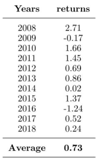
Table 1 displays the averages of monthly percent returns for the environmental
factor, GMC, for each year from 2008 to 2018. We can see that at the very beginning
of phase II of EU-ETS (2008), GMC is positive (+2.71%). It is slightly negative in
2009 and then picks up in 2010 (+1.66%), 2011 (+1.45%), 2012 (+0.69%), and 2013
(+0.86%, beginning of phase III), it lowers to almost zero in 2014 (+0.02%) and then
picks up again in 2015 (+1.37%). It then drops in 2016 (-1.24%), which singularly is
starts to increase slowly from 2017 onwards. There is a clear path in the magnitude
of GMC, starting from the beginning of phase II in 2008 and which is only stopped
in 2016 by, we suppose, a market negatively perceived COP 21 outcome. Over the
11-year span the average monthly percent return for the GMC factor is 0.73%.
Table 1. Average monthly GMC percent return from 2008 to 2018
Years returns 2008 2.71 2009 -0.17 2010 1.66 2011 1.45 2012 0.69 2013 0.86 2014 0.02 2015 1.37 2016 -1.24 2017 0.52 2018 0.24 Average 0.73
Table 1 provides an argument to test a 5+1 version of Fama and French’s (2015)
five factor model and see if the augmented model outperforms — in Europe in the
2008-2018 time span — the classical one. The 5+1 model specification, which we call
EE-FF (environmentally-extended Fama and French) model is the following:
Ri,t−RF,t= αi+βi(RM,t−RF,t)+siSM Bt+hiHM Lt+riRM Wt+ciCM At+giGM Ct+ei,t
(2)
3. The data
The EE-FF model (2) aims at capturing patterns in average returns related to size,
value, profitability, investment and EU-ETS compliance. The explanatory variables
include the returns on a market portfolio of European stocks, RM, and mimicking
portfolios for the size, SM B, value, HM L, profitability, RM W , investment, CM A,
and EU-ETS compliance, GM C, factors in returns. The returns to be explained are
which the GMC factor is based. Such subsets are formed by breaking up the 182 firms
into 8 portfolios based on market capitalization and EU-ETS compliance: the 8 stock
portfolios are formed from annual (2008-2018) sorts of stocks into 4 size groups (4
quartiles) and two EU-ETS groups — liable firms, which we call carbon, and exempt
firms, which we call green —. Liable firms participate to the EU-ETS in the
2008-2018 time frame while exempt firms do not participate. The risk free rate, RF, is the
1-month Euribor rate.
3.1. Explanatory returns
The 5 classical factors —RM, SM B, HM L, RM W, CM A— are taken directly from
Fama and French’s database of factors for the European market. For a complete
de-scription of the construction of the factors we refer the reader to Fama and French
(2015): here it suffices to mention that the 5 classical factors (2x3) are constructed
using 6 value-weight portfolios formed on size and book-to-market, 6 value-weight
port-folios formed on size and operating profitability, and 6 value-weight portport-folios formed
on size and investment. All the portfolios are shuffled on a yearly basis. SMB (small
minus big) is the average return on the nine small stock portfolios minus the average
return on the nine big stock portfolios, HML (high minus low) is the average return on
the two value portfolios minus the average return on the two growth portfolios, RMW
(robust minus weak) is the average return on the two robust operating profitability
portfolios minus the average return on the two weak operating profitability portfolios,
CMA (conservative minus aggressive) is the average return on the two conservative
investment portfolios minus the average return on the two aggressive investment
port-folios, while RM is the return on Europe’s value-weight market portfolio.
The environmental factor, GMC (green minus carbon), is constructed using a
port-folio of 182 European stocks, out of which 91 participate to the EU-ETS since the
beginning of phase II (2008) and 91 do not participate to the EU-ETS since the
begin-ning of phase II. A firm participates to the EU-ETS since the beginbegin-ning of phase II if
it belongs to one of the following sectors: power stations and other combustion plants
> 20M W , oil refineries, coke ovens, iron and steel plants, cement clinker, glass, lime,
liable group of firms (“carbon” firms) is formed on the following three criteria: a)
be-longing to the sectors that take part to the EU-ETS since the beginning of phase II
(2008), b) having at least one installation listed in the EU-ETS transaction log, and
c) listing on a European stock exchange of the countries participating to the EU-ETS,
i.e. the EU countries plus Iceland, Liechtenstein and Norway. We consider firms to be
“green”, i.e. EU-ETS exempt, if the following three criteria are met: a) belonging to
the sectors which do not take part to the EU-ETS since the beginning of phase II, b)
no firm installations are inventoried on the EU-ETS transaction log, and c) the firm
is listed on a European stock exchange of the countries participating to the EU-ETS.
Two portfolios, comprising in one case stocks of carbon firms and, in the other,
stocks of green firms, have been formed from January 2008 to December 2018. The
portfolios do not need to be shuffled on a yearly basis since the 182 European firms
that are under examination constantly participate (or not) to the EU-ETS in the
2008-2018 time frame. Monthly value-weight stock returns have been calculated for the two
portfolios for the 11-year time frame for a total of 24,024 observations. Lastly, GMC
is obtained by subtracting the monthly value-weight carbon portfolio return from the
monthly value-weight green portfolio return.
3.2. Explained returns
In the EE-FF model (2), the returns to be explained, Ri, are the value weight returns
for subsets of the portfolio of 182 European stocks upon which the GMC factor is based.
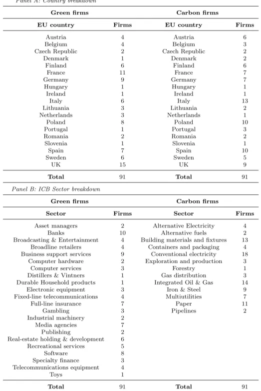
Descriptive statistics for the 182 European stock portfolio are provided in Table 2.
Such subsets are formed from annual (2008-2018) sorts of stocks into 4 size groups
(4 quartiles) and 2 EU-ETS compliance groups: EU-ETS liability and EU-ETS
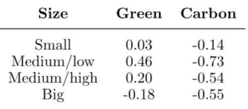
exemp-tion. Table 3 shows the average monthly value-weight excess returns for the 8 portfolios
obtained from annual sorts of the 182 European stocks into 4 size groups (4 quartiles)
and two EU-ETS compliance groups. Once again, we call the portfolio “carbon” if it
includes firms that do participate to the EU-ETS, and we call the portfolio “green” if
it includes firms which do not take part to the EU-ETS. Here, average return typically
falls from small stocks to big stocks, i.e. there is a clear size effect pattern. Even though
Table 2. Descriptive statistics for the 182 European stocks: country and sector (ICB) breakdown for Carbon and Green firms
Panel A: Country breakdown
Green firms Carbon firms
EU country Firms EU country Firms
Austria 4 Austria 6
Belgium 4 Belgium 3
Czech Republic 2 Czech Republic 2
Denmark 1 Denmark 2 Finland 6 Finland 6 France 11 France 7 Germany 9 Germany 7 Hungary 1 Hungary 1 Ireland 1 Ireland 1 Italy 6 Italy 13 Lithuania 3 Lithuania 2 Netherlands 3 Netherlands 1 Poland 8 Poland 10 Portugal 1 Portugal 3 Romania 2 Romania 2 Slovenia 1 Slovenia 1 Spain 7 Spain 10 Sweden 6 Sweden 5 UK 15 UK 9 Total 91 Total 91
Panel B: ICB Sector breakdown
Green firms Carbon firms
Sector Firms Sector Firms Asset managers 2 Alternative Electricity 4
Banks 10 Alternative fuels 2 Broadcasting & Entertainment 4 Building materials and fixtures 13
Broadline retailers 4 Containers and packaging 4 Business support services 9 Conventional electricity 18
Computer hardware 2 Exploration and production 3 Computer services 3 Forestry 1 Distillers & Vintners 1 Gas distribution 3 Durable Household products 1 Integrated Oil & Gas 14
Electronic equipment 3 Iron & Steel 9 Fixed-line telecommunications 4 Multiutilities 7 Full-line insurance 7 Paper 11
Gambling 3 Pipelines 2
Industrial machinery 2 Media agencies 7 Publishing 2 Real-estate holding & development 6 Recreational services 5 Software 8 Specialty finance 3 Telecommunications equipment 4 Toys 1 Total 91 Total 91
the first to the fourth quartile. This holds both in the case of carbon stocks and in the
case of green stocks. What matters to us, rather that the size effect, which has been
the size effect: the green portfolio systematically outperforms its carbon counterpart
at each size level.
Table 3. Averages of monthly percent excess returns for 8 value-weight portfolios formed from sorts on size and EU-ETS compliance. January 2008-December 2018.
Size Green Carbon Small 0.03 -0.14 Medium/low 0.46 -0.73 Medium/high 0.20 -0.54 Big -0.18 -0.55
4. Results
The classical Fama and French’s (1) five factor model and the EE-FF model (2) have
been run for each dependent variable for a total of 16 time-series regressions. There
is direct evidence that the addition of a sixth factor improves the effectiveness of the
classical five factor model, at least in Europe in the 2008-2018 time span. Overall, the
slopes and the R2 values obtained with the EE-FF model are direct evidence of the impact of the EU-ETS (low-carbon policy) upon European stock returns.
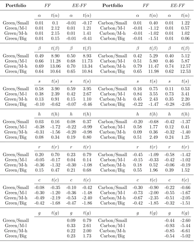
Table 4 displays the results of the 8 regressions, one for each response variable,
that have been run with five explicatory variables — RM, SM B, HM L, RM W, CM A
— and of the 8 regressions which have been run with six explicatory variables —
RM, SM B, HM L, RM W, CM A, GM C— . The response variables are the monthly
value weight excess returns of the eight portfolios formed from annual sorts of the 182
European stocks into 4 size groups (4 quartiles) and two EU-ETS groups (liable and
exempt).
The adjusted R2 values for the original Fama and French (FF) model fall in between the 0.31-0.72 range, meaning that the FF model fares quite well in the representation
of the variance of the outcome variables, at least in Europe in the 2008-2018 time
frame. The 0.31 R2 value comes from the small cap/carbon portfolio regression, while the second lowest R2 value is 0.51 (medium-low cap/carbon), which is followed by an R2 value of 0.54 (small cap/green). All other R2 values are above 0.64.
Table 4. Results of the regressions carried out with the five factor model (FF) and the EE-FF for 8 value-weight portfolios formed on size and EU-ETS participation. January 2008-December 2018.
Portfolio FF EE-FF Portfolio FF EE-FF
α t(α) α t(α) α t(α) α t(α) Green/Small 0.01 0.1 -0.01 -0.17 Carbon/Small 0.01 0.40 0.01 1.22 Green/M-l 0.01 2.12 0.01 1.21 Carbon/M-l -0.01 -1.12 0.01 0.57 Green/M-h 0.01 2.15 0.01 1.41 Carbon/M-h -0.01 -1.02 0.01 1.02 Green/Big 0.01 0.15 -0.01 -0.41 Carbon/Big -0.01 -1.51 0.01 0.06 β t(β) β t(β) β t(β) β t(β) Green/Small 0.49 8.90 0.50 8.93 Carbon/Small 0.42 5.29 0.40 5.12 Green/M-l 0.66 11.28 0.68 11.73 Carbon/M-l 0.51 5.80 0.46 5.87 Green/M-h 0.69 13.06 0.70 13.34 Carbon/M-h 0.79 11.47 0.74 12.57 Green/Big 0.64 10.64 0.65 10.84 Carbon/Big 0.65 11.98 0.62 12.53 s t(s) s t(s) s t(s) s t(s) Green/Small 0.58 3.90 0.59 3.95 Carbon/Small 0.16 0.75 0.11 0.53 Green/M-l 0.38 2.39 0.42 2.67 Carbon/M-l 0.84 3.55 0.73 3.41 Green/M-h 0.13 0.91 0.15 1.10 Carbon/M-h 0.45 2.43 0.35 2.20 Green/Big -0.10 -0.62 -0.07 -0.46 Carbon/Big -0.22 -1.47 -0.28 -2.05 h t(h) h t(h) h t(h) h t(h) Green/Small 0.03 0.16 0.08 0.37 Carbon/Small -0.20 -0.68 -0.42 -1.37 Green/M-l -0.38 -1.72 -0.22 -0.99 Carbon/M-l 0.58 1.77 0.12 0.41 Green/M-h -0.31 -1.56 -0.20 -0.98 Carbon/M-h 0.09 0.36 -0.32 -1.40 Green/Big 0.08 0.34 0.19 0.80 Carbon/Big 0.51 2.49 0.24 1.25 r t(r) r t(r) r t(r) r t(r) Green/Small 0.20 0.70 0.23 0.79 Carbon/Small -0.45 -1.09 -0.58 -1.42 Green/M-l -0.05 -0.17 0.04 0.14 Carbon/M-l -0.15 -0.33 -0.42 -1.02 Green/M-h -0.36 -1.32 -0.30 -1.08 Carbon/M-h 0.18 0.52 -0.06 -0.19 Green/Big 0.15 0.47 0.21 0.68 Carbon/Big 0.55 1.96 0.39 1.52 c t(c) c t(c) c t(c) c t(c) Green/Small -0.08 -0.35 -0.10 -0.42 Carbon/Small -0.30 -0.90 -0.22 -0.66 Green/M-l -0.30 -1.20 -0.36 -1.48 Carbon/M-l -0.73 -2.00 -0.55 -1.67 Green/M-h -0.49 -2.19 -0.53 -2.40 Carbon/M-h -0.67 -2.35 -0.51 -2.05 Green/Big -0.42 -1.68 -0.47 -1.86 Carbon/Big -0.42 -1.85 -0.32 -1.51 g t(g) g t(g) g t(g) g t(g) Green/Small 0.09 0.79 Carbon/Small -0.44 -2.60 Green/M-l 0.33 2.61 Carbon/M-l -0.93 -5.44 Green/M-h 0.22 2.00 Carbon/M-h -0.85 -6.61 Green/Big 0.23 1.73 Carbon/Big -0.54 -5.02
the FF model are almost indistinguishable from zero — the lowest being -0.01 and
the highest being 0.01 — and 2 intercepts out of 8 are statistically significant at the
0.05 level. Fama and French (2015) suggest two interpretations of the zero-intercept
returns and interpreting the factor model as the regression equation of Merton’s (1973)
model in which unspecified state variables lead to risk premiums that are not captured
by the market factor. If the coefficients of the time-series regression —βi, si, hi, ri, ci
— completely capture variation in expected returns, then the intercept, αi, is
indistin-guishable from zero. Under the assumption of the zero-intercept hypothesis, the range
of values obtained for the intercepts provide evidence of the accuracy of the FF model
to represent the financial reality under analysis.
Table 4 also shows coefficients and t -statistics for the five factors. While the market
factor is always highly statistically significant, the size factor is significant at the
0.05 level in 4 out of 8 cases (small cap/green, medium-low cap/green, medium-low
cap/carbon, medium-high cap/carbon). The value factor is statistically significant at
the 0.05 level in one case out of eight (big cap/carbon) and the investment factor —
CMA— in three out of eight cases (medium-high cap/green, medium-low cap/carbon,
medium-high cap/carbon).
The EE-FF model finds adjusted R2 values in the 0.34-0.76 range. The regressions carried out with the EE-FF model find adjusted R2 values which are larger is 6 cases out of 8 than the regressions carried out with the classical FF model. The only R2 values which do not improve in the passage from a five factor model to a six factor
model come from the small cap/green regression and the big cap/green regression. In
these two cases the adjusted R2 values are exactly the same for the FF model and the EE-FF model.
We find highly statistically significant coefficients for the GMC factor in 6
regres-sions out of 8, the only exception being the small cap/green portfolio (t-statistic=0.79)
and the big cap/green portfolio (t-statistic= 1.73). As expected, coefficients are
posi-tive when the dependent variable is a green (i.e. does not participate to the EU-ETS)
portfolio and negative when the dependent variable is a carbon (i.e. does participate to
the EU-ETS) portfolio. GMC’s positive coefficients range from 0.09 (small cap/green)
to 0.33 (medium-low cap/green), whereas GMC’s negative coefficients range from -0.44
(small cap/carbon) to -0.93 (medium-low cap/carbon).
Again, the GMC coefficient for the small cap/green portfolio (0.79) and the big
sta-tistically significant at the 0.05 level. Additionally, the magnitude of the coefficients of
the green portfolios are evidently lower than their carbon counterparts, i.e. firms are
more penalized for their participation to the EU-ETS rather than rewarded for their
exemption from the EU-ETS. We suspect this is due to the fact that there are some
sectors which are considered as carbon-intensive by the market but which are not yet
included in the EU-ETS participant list. Armed with statistical evidence, we conclude
it is legitimate to consider the addition of the GMC factor to the classical Fama and
French’s five factors in Europe, at least from 2008.
5. Redundant factors
The previous section has shown that the inclusion of a sixth factor —GMC— improves
the effectiveness of Fama and French’s five factor model in Europe from 2008 onwards.
Nevertheless, such addition may hinder the explication power of the classical five
factors, i.e. the portion of variance in returns explained by a “classical” factor may be
partially absorbed by the GMC factor we are putting forward. As such addition may
lead to a factor redundancy, we perform a principal component analysis (PCA) on the
5+1 factors in order to figure out how many factors to include in the regression of the
returns to be explained, Ri− RF.
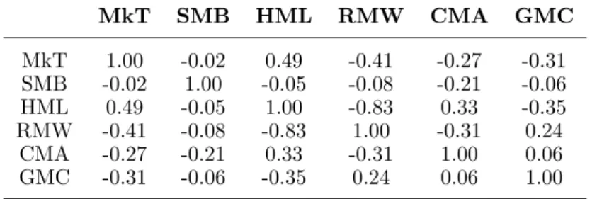
Table 5 shows the correlations matrix between the 6 factors. Noticeable correlations
are shown between RM, or M kT , and HM L (0.49), between RM W and HM L (-0.83)
and between RM W and RM (-0.41).
Table 5. Correlation Matrix for the market, size, value, profitability, investment and EU-ETS factor
MkT SMB HML RMW CMA GMC MkT 1.00 -0.02 0.49 -0.41 -0.27 -0.31 SMB -0.02 1.00 -0.05 -0.08 -0.21 -0.06 HML 0.49 -0.05 1.00 -0.83 0.33 -0.35 RMW -0.41 -0.08 -0.83 1.00 -0.31 0.24 CMA -0.27 -0.21 0.33 -0.31 1.00 0.06 GMC -0.31 -0.06 -0.35 0.24 0.06 1.00
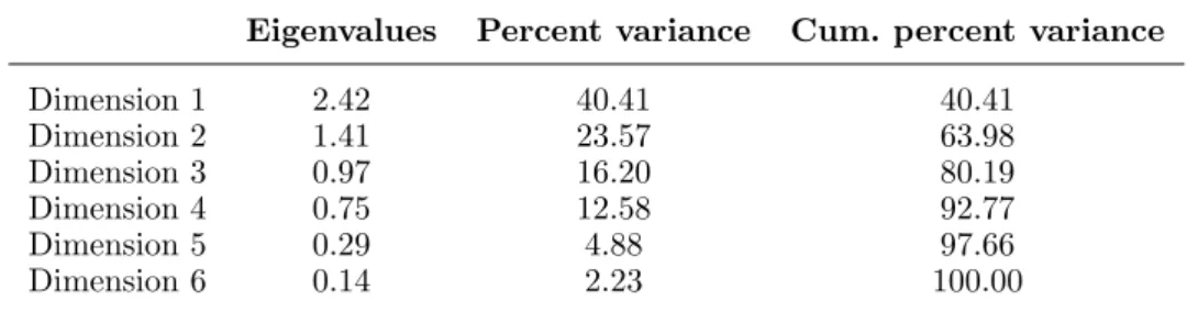
Table 6 displays the eigenvalues and the proportion of variances retained by the
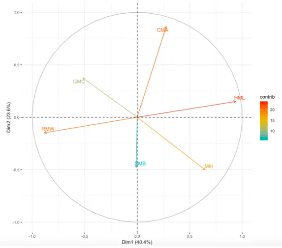
principal components. If we were to follow Kaiser’s rule we would have to retain
between RM W and HM L and the relative low contribution of SM B to the two main
principal components (figure 1), these would be natural candidates to the discarded.
Unfortunately, figure 1 shows that the contribution of CMA is superior to that of
GMC. Ultimately, if we were to follow Kaiser’s rule we would just settle for the market
factor, RM (M kT ), and the investment factor, CM A. As this choice is not coherent
with our research objective, we decide not to follow Kaiser’s rule and settle for three
components which account for 80% of the total variance: RM (M kT ), CM A and
GM C. The reduced version of the EE-FF model, then, becomes:
Ri,t− RF,t= αi+ βi(RM,t− RF,t) + ciCM At+ giGM Ct+ ei,t (3)
Table 6. Eigenvalues, variance and cumulative variance for the 6 components
Eigenvalues Percent variance Cum. percent variance
Dimension 1 2.42 40.41 40.41 Dimension 2 1.41 23.57 63.98 Dimension 3 0.97 16.20 80.19 Dimension 4 0.75 12.58 92.77 Dimension 5 0.29 4.88 97.66 Dimension 6 0.14 2.23 100.00
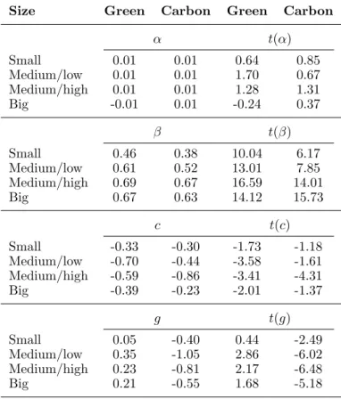
Table 7 displays the results of the 8 regressions, one for each response variable, that
have been run with three explicatory variables — RM, CM A, GM C —. The response
variables are the monthly value weight excess returns of the eight portfolios formed
from annual sorts of the 182 European stocks into 4 size groups (4 quartiles) and two
EU-ETS groups (liable and exempt).
A comparison of table 4 — the EE-FF with 6 factors— and table 7 — EE-FF
with 3 factors — shows that reducing the number of factors improves t -values for the
intercepts in five cases out of eight. On the other hand reducing the number of factors
increases the statistical significance of the market coefficient for eight portfolios out
of eight and of the investment coefficient for six portfolios out of eight. With regard
to the GMC coefficient, moving on from 6 to 3 factors only improves the statistical
Figure 1. Contributions of MkT, SMB, HML, RMW, CMA and GMC variables to the two first dimensions
with 3 factors (table 7) only improve over the adjusted R2 values of the EE-FF with 6 factors (table 4) in one case out of eight: the big cap/green portfolio. The adjusted
R2 values for the other portfolios are exactly identical or slightly inferior. Overall, we find that the reduced version of the EE-FF model (3 factors), while leading to some
moderate statistical improvements over the EE-FF model with 6 factors, partially loses
Table 7. Results of the regressions for 8 value-weight portfolios formed on size and EU-ETS participation carried out with the 3 factor EE-FF model. January 2008-December 2018.
Size Green Carbon Green Carbon
α t(α) Small 0.01 0.01 0.64 0.85 Medium/low 0.01 0.01 1.70 0.67 Medium/high 0.01 0.01 1.28 1.31 Big -0.01 0.01 -0.24 0.37 β t(β) Small 0.46 0.38 10.04 6.17 Medium/low 0.61 0.52 13.01 7.85 Medium/high 0.69 0.67 16.59 14.01 Big 0.67 0.63 14.12 15.73 c t(c) Small -0.33 -0.30 -1.73 -1.18 Medium/low -0.70 -0.44 -3.58 -1.61 Medium/high -0.59 -0.86 -3.41 -4.31 Big -0.39 -0.23 -2.01 -1.37 g t(g) Small 0.05 -0.40 0.44 -2.49 Medium/low 0.35 -1.05 2.86 -6.02 Medium/high 0.23 -0.81 2.17 -6.48 Big 0.21 -0.55 1.68 -5.18
6. The carbon stress test
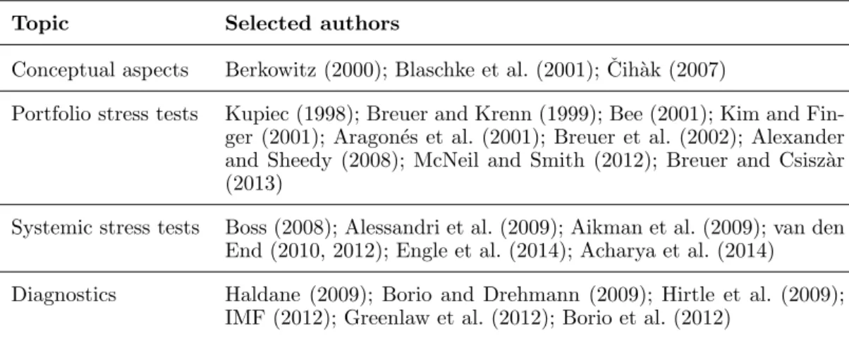
The financial stress test literature, following Koliai (2016), can be split in four main
categories (table 8): general presentation of the instrument in the early 2000s, portfolio
stress test development, systemic stress test emergence in the wake of the 2007-2009
crisis and diagnosis of the realized exercises.
The literature, while portraying stress testing as quintessential to financial risk
management (Bensoussan, Guegan, & Tapiero, 2014), describes the technique through
dichotomies: top-down and bottom-up approaches, first and second round effects,
sen-sitivity and scenario analysis, historical and hypothetical scenarios, direct and reverse
stress tests. In the top-down approaches the empirical relationship between a banking
variable and an exogenous stressor is assumed at the portfolio level of low granularity,
while in the bottom-up approach the empirical relationship is estimated at the highest
possible level of granularity of a banking variable.1 First-round effects come from the immediate impact of the shock on the financial system, while second-round effects
Table 8. Categorisation of stress test literature (Koliai, 2016)
Topic Selected authors
Conceptual aspects Berkowitz (2000); Blaschke et al. (2001); ˇCih`ak (2007)
Portfolio stress tests Kupiec (1998); Breuer and Krenn (1999); Bee (2001); Kim and Fin-ger (2001); Aragon´es et al. (2001); Breuer et al. (2002); Alexander and Sheedy (2008); McNeil and Smith (2012); Breuer and Csisz`ar (2013)
Systemic stress tests Boss (2008); Alessandri et al. (2009); Aikman et al. (2009); van den End (2010, 2012); Engle et al. (2014); Acharya et al. (2014) Diagnostics Haldane (2009); Borio and Drehmann (2009); Hirtle et al. (2009);
IMF (2012); Greenlaw et al. (2012); Borio et al. (2012)
include “possible domino effects from the institutions that are directly affected by the
shock to other intermediaries and, possibly, to market infrastructures and the entire
financial system” (Quagliariello, 2009, p.33). Sensitivity testing aims at determining
how changes to a single risk factor will impact the institution or the portfolio while
scenario analysis studies the effect of a simultaneous move in a group of risk factors.
Scenarios have been subjects to requirements by the Basel Committee on Banking
Supervision (2009) which demands them to be plausible but severe: historical
scenar-ios rely on a significant market event experienced in the past, whereas a hypothetical
scenario is a significant market event that has not yet happened (Committee on the
Global Financial System, 2005). Direct stress tests set scenarios and derive losses,
while “starting from a big loss and working backward to identify how such a loss
would occur is commonly referred to among risk management professionals as reverse
stress testing” (Breuer, Jandaˇcka, Menc´ıa, & Summer, 2012, p. 332).
The carbon stress test we put forward is based on the GMC factor obtained with
the EE-FF model (6 factors). The GMC is a proxy that mimics the risk factor in
returns related to the payment of a carbon price and its coefficient —in the EE-FF
model — is interpreted as the average effect on stock returns of a one unit increase
in GMC holding all other predictors fixed. It follows that, if GMC increases, the risk
factor related to participating to the EU-ETS raises accordingly. Conversely, if GMC
decreases, the risk factor related to participating to the EU-ETS diminishes. It is
a carbon risk factor decrease goes with a lower EU-ETS price. In order to understand
the impact of a hypothetical, but plausible and severe, EU-ETS price upon the stock
returns under examination, we stress the average GMC portfolio value by 20% (low
shock), 50% (medium shock), and 100% (high shock) and we look at the effect on each
of the 8 value-weight portfolios formed from annual sorts of the 182 European stocks
into 4 size groups (4 quartiles) and two EU-ETS compliance groups (liable, or carbon,
and exempt, or green).
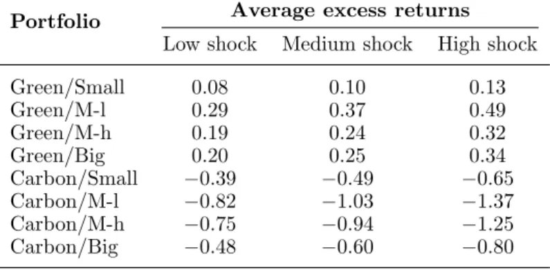
Table 9. 11-year (2008-2018) average monthly percent excess returns explained by the GMC factor for stressed values of GMC.
Portfolio Average excess returns Low shock Medium shock High shock Green/Small 0.08 0.10 0.13 Green/M-l 0.29 0.37 0.49 Green/M-h 0.19 0.24 0.32 Green/Big 0.20 0.25 0.34 Carbon/Small −0.39 −0.49 −0.65 Carbon/M-l −0.82 −1.03 −1.37 Carbon/M-h −0.75 −0.94 −1.25 Carbon/Big −0.48 −0.60 −0.80
Table 9 shows the results of the carbon stress test for each of the 8 value-weight
portfolios for the three shock scenarios: the second, third and fourth column provide the
averages of monthly percent excess returns explained by the GMC factor for stressed
values of GMC. Results of the carbon stress test show the magnitude of the increase
(decrease) of average excess stock returns for green firms (carbon firms) in case of an
average ETS price appreciation of 20% (low shock), 50% (medium shock), and 100%
(high shock) for each market cap tranche.
7. Conclusions
Changes in extreme climate phenomena such as temperature extremes, high sea levels
extremes or precipitation extremes are likely to seriously affect several facets of natural
and human systems. There is scientific evidence that human activity, by altering the
composition of the atmosphere, contributes to global warming. Addressing climate
autonomous, it is mostly carried out with policy, i.e. low-carbon policy. This leads to
the research question of the effect of low-carbon policy upon financial values. In the
context of EU-ETS, this question has found contradictory results: some studies find
the impact of this low-carbon policy on financial values beneficial, some others find it
detrimental.
The objective of this paper is to study the impact of low-carbon policy upon the
value of financial assets, particularly stock returns. Specifically, we seek to understand
and explain the impact of one particular European policy, the 2003/87/CE
direc-tive upon which the EU-ETS is based, upon European stock returns. To answer this
question, we selected 182 European firms that fall in two categories: firms that do
participate to the EU-ETS (carbon firms) and firms that do not participate to the
EU-ETS (green firms) since the beginning of phase II (2008). With 11 years of data
(2008-2018) we use a multi-factor model inspired by Fama and French (2015) whose
key new component is an EU-ETS compliance factor, GMC (green minus carbon). The
GMC portfolio is obtained by subtracting the monthly value-weight carbon portfolio
returns from the monthly value-weight green portfolio returns.
Following our analysis, results show that, just as there are patterns in average
returns related to size, profitability and investment, which have been proven elsewhere,
there is also a pattern related to EU-ETS compliance. Such pattern exists, in Europe,
since the implementation of EU-ETS: there is a high green premium, rather than a
carbon premium like parts of the literature asserted previously, and this green premium
is highly statistically significant, i.e. green stocks outperform on average carbon stocks
over the 11-year span. Furthermore, we follow the recent carbon stress test trend by
putting forward a stress test able to indicate what is the impact of a hypothetical
EU-ETS price upon stock returns: our results show the effects of a plausible but more
severe average EU-ETS price on both carbon firms and green firms for each market
cap tranche.
These results are also the basis for the policy implications for legislators and financial
practitioners. Our findings show that the 2003/87/CE directive has a positive effect
in the financing of the low-carbon transition: the beginning of phase II of EU-ETS
high-carbon firms and capital inflows to low-high-carbon firms. The high-carbon stress test we put
forward shows by how much an increase of the EU-ETS price would accelerate such
process. The low-shock scenario, for example, would provide an additional boost to the
low-carbon transition without harming excessively high-carbon firms. From a financial
practitioner perspective, our findings show that, in Europe, in the 2008-2018 time span,
low-carbon firms have outperformed high-carbon firms and that this outperformance is
statistically significant. In other words, low-carbon investments cannot be considered
anymore just an ethical stand: nowadays, as the green premium shows, investing in
low-carbon firms is a profitable exercise.
Acknowledgements
The author would like to acknowledge the feedbacks obtained at the conferences where
previous versions of this article were presented.
Disclosure statement
The author declares no potential conflict of interest.
Notes
1The division refers to the US definitions whereas in Europe top-down refers to stress tests carried out by regulators and bottom-up by banks
References
[1] Bank of England Prudential Regulation Authority. (2015). The impact of climate change on the UK insurance sector. A Climate Change Adaptation Report by the Prudential Regulation Authority. Re-trieved from https://www.bankofengland.co.uk/prudential-regulation/publication/2015/the-impact-of-climate-change-on-the-uk-insurance-sector
[2] Basel Committee on Banking Supervision. (2009). Principles for sound stress testing practices and su-pervision. Retrieved fromhttps://www.bis.org/publ/bcbs155.htm
[3] Battiston, S., Mandel, A., Monasterolo, I., Sch¨utze, F., & Visentin, G. (2017). A climate stress-test of the financial system. Nature Climate Change, 7 (4), 283-288.doi:10.1038/nclimate3255
[4] Bensoussan, A., Guegan, D., & Tapiero, C. S. (2014). Future Perspectives in Risk Models and Finance. Cham: Springer.
[5] Bernardini, E., Di Giampaolo, J., Faiella, I., & Poli, R. (2019). The impact of carbon risk on stock returns: evidence from the European electric utilities. Journal of Sustainable Finance & Investment.
https://doi.org/10.1080/20430795.2019.1569445
[6] Borio, C., Drehmann, M., & Tsatsaronis, K. (2014). Stress-testing macro stress testing: does it live up to expectations? Journal of Financial Stability, 12, 3-15.doi:10.1016/j.jfs.2013.06.001
[7] Breuer, T., Jandaˇcka, M., Menc´ıa, J., & Summer, M. (2012). A systematic approach to multi-period stress testing of portfolio credit risk. Journal of Banking & Finance, 36 (2), 332-340.
doi:10.1016/j.jbankfin.2011.07.009
[8] Brouwers, R., Schoubben, F., Van Hulle, C., & Van Uytbergen, S. (2016). The ini-tial impact of EU ETS verification events on stock prices. Energy policy, 94, 138-149.
https://doi.org/10.1016/j.enpol.2016.04.006
[9] Caldecott, B., & McDaniels, J. (2014). Financial dynamics of the environment: Risks, impacts, and barriers to resilience. Oxford: Smith School of Enterprise and the Environment.
[10] Carhart, M. M. (1997). On persistence in mutual fund performance. The Journal of finance,52 (1), 57-82.
doi.org/10.1111/j.1540-6261.1997.tb03808.x
[11] Caldecott, B., Kruitwagen, L., Dericks, G., Tulloch, D. J., Kok, I., & Mitchell, J. (2016). Stranded Assets and Thermal Coal: An analysis of environment-related risk exposure. Oxford: Smith School of Enterprise and the Environment.
[12] Cambridge Centre for Sustainable Finance. (2016). Environmental risk analysis by financial institutions: a review of global practice. Retrieved from https://www.cisl.cam.ac.uk/publications/sustainable-finance-publications/environmental-risk-analysis-by-financial-institutions-a-review-of-global-practice
[13] Carney, M. (2015). Breaking the tragedy of the horizon—climate change and financial stability. Retrieved from https://www.bankofengland.co.uk/speech/2015/breaking-the-tragedy-of-the-horizon-climate-change-and-financial-stability
[14] Committee on the Global Financial System. (2005). Stress Testing at Major Financial Institutions: survey results and practice. Retrieved fromhttps://www.bis.org/publ/cgfs24.htm
[15] Dell, M., Jones, B. F., & Olken, B. A. (2014). What do we learn from the weather? The new climate-economy literature. Journal of Economic Literature, 52 (3), 740-798.doi:10.1257/jel.52.3.740
[16] European Commission. (2015). EU-ETS handbook. Retrieved from European Commission website:
https://ec.europa.eu/clima/publications
[17] Fama, E. F., & French, K.R. (1993). Common risk factors in the returns on stocks and bonds. Journal of Financial Economics, 33 (1), 3-56.https://doi.org/10.1016/0304-405X(93)90023-5
[18] Fama, E. F., & French, K.R. (2015). A five-factor asset pricing model. Journal of Financial Economics, 116 (1), 1-22.https://doi.org/10.1016/j.jfineco.2014.10.010
[19] Fay, M., Hallegatte, S., Vogt-Schilb, A., Rozenberg, J., Narloch, U., & Kerr, T. (2015). Decarbonizing development: Three steps to a zero-carbon future. Washington, DC: World Bank
[20] G¨orgen, M., Jacob, A., Nerlinger, M., Riordan, R., Rohleder, M., & Wilkens, M. (2017). Carbon risk. Retrieved fromhttps://papers.ssrn.com/sol3/papers.cfm?abstractid = 2930897
[21] Graff Zivin, J., & Neidell, M. (2014). Temperature and the allocation of time: Implications for climate change. Journal of Labour Economics, 32 (1), 1-26.doi:10.1086/671766
[22] Hallegatte, S., Fay, M., Bangalore, M., Kane, T., & Bonzanigo, L. (2015). Shock waves: managing the impacts of climate change on poverty. Washington, DC: World Bank
[23] Industrial and Commercial Bank of China. (2016). Impact of Environmental Factors on Credit Risk of Commercial Banks. Beijing: ICBC.
[24] Intergovernmental Panel on Climate Change. (2014). Climate Change 2014: Synthesis Report. Retrieved fromhttp://www.ipcc.ch/report/ar5/syr/
[25] Koch, N., & Bassen, A. (2013). Valuing the carbon exposure of European utilities. The role of fuel mix, permit allocation and replacement investments. Energy Economics, 36, 431-443.
doi:10.1016/j.eneco.2012.09.019
[26] Koliai, L. (2016). Extreme risk modeling: An EVT pair copulas approach for financial stress tests. Journal of Banking & Finance, 70, 1-22.doi:10.1016/j.jbankfin.2016.02.004
[27] Moreno, B., & Pereira da Silva, P. (2016). How do Spanish polluting sectors’ stock market re-turns react to European Union allowances prices? A panel data approach. Energy, 103 (15), 240-250.
https://doi.org/10.1016/j.energy.2016.02.094
[28] Nguyen Anh Pham, H., Ramiah, V., & Moosa, I. (2019). The effects of environmental regulation on the stock market: the French experience. Accounting & Finance.https://doi.org/10.1111/acfi.12469
[29] Oestreich, A. M., & Tsiakas, I. (2015). Carbon emissions and stock returns: Evidence from the EU Emis-sions Trading Scheme. Journal of Banking & Finance, 58, 294-308.doi:10.1016/j.jbankfin.2015.05.005
[30] Pycroft, J., Abrell, J., & Ciscar, J. C. (2016). The global impacts of extreme sea-level rise: a comprehensive economic assessment. Environmental and Resource Economics, 64 (2), 225-253. doi:10.1007/s10640-014-9866-9
[31] Quagliariello, M. (2009). Stress-testing the banking system: methodologies and applications. New York: Cambridge University Press.
[32] Schoenmaker, D., & van Tilburg, R. (2016). Financial risks and opportunities in the time of climate change. Brussels: Bruegel.
[33] Tian, Y., Akimov, A., Roca, E., & Wong, V. (2015). Does the carbon market help or hurt the stock price of electricity companies? Further evidence from the European context. Journal of Cleaner Production, 112 (2),1619-1626.https://doi.org/10.1016/j.jclepro.2015.07.028
[34] Zenghelis, D., & Stern, N. (2016). The importance of looking forward to manage risks: submission to the Task Force on Climate-Related Financial Disclosures. Retrieved from
http://www.lse.ac.uk/GranthamInstitute/publication/the-importance-of-looking-forward-to-manage-risks-submission-to-the-task-force-on-climate-related-financial-disclosures/
[35] Zhang, F., Fang, H., & Wang, X. (2018). Impact of Carbon Prices on Corporate Value: The Case of China’s Thermal Listed Enterprises. Sustainability,10 (9), 3328.https://doi.org/10.3390/su10093328
[36] Zhang, M., & Gregory-Allen, R.B. (2018). Carbon Emissions and Stock Returns: Evidence from the Chinese Pilot Emissions Trading Scheme. Theoretical Economics Letters, 8 (11), 2082-2094.
https://doi.org/10.4236/tel.2018.811136
[37] Zhou, Z., Xiao, T., Chen, X., & Wang, C. (2016). A carbon risk prediction model for Chinese heavy-polluting industrial enterprises based on support vector machine. Chaos, Solitons & Fractals, 89, 304-315.
doi:10.1016/j.chaos.2015.12.001
[38] Zhu, H., Tang, Y., Peng, C., & Yu, K. (2018). The heterogeneous response of the stock market to emission allowance price: evidence from quantile regression. Carbon Management, 9 (3), 277-289.