DYPHORA—a dynamic model for the rate of photosynthesis of algae

DYPHORA—a dynamic model for the rate of photosynthesis of

algae

C.Pahl-Wostl and D.M.Imboden

Swiss Federal Institute of Technology Zurich, Environmental Physics, Institute for Aquatic Sciences and Water Pollution Control, do EAWAG, CH-8600

Dubendorf, Switzerland

Abstract. Experimental data obtained from different cultures of phytoplankton indicate that photosynthesis (F) depends on light intensity (I) in a dynamic way. Therefore, static Pll curves relating photosynthesis to the instantaneous light may not be adequate to describe the activity of algal cells in lakes or oceans where mixing can cause a complex pattern of light variation. The model DYPHORA (DYnamic model for the PHOtosynthetic Rate of Algae) describes the response of photosynthesis to light using two characteristic times, the response time to increasing light (Tr), and

the light inhibition decay time (T,). The model agrees well with available experiments if T, is chosen between 0.5 and 5 min, and T, between 30 and 120 min. It explains the occurrence of the well-documented afternoon depression as well as the decrease of integrated long-term rates of photosynthesis with increasing light. Although the presented comparison of experimental data and model results cannot serve as a proof for DYPHORA in a strict sense, the structural relationship between P and / can nevertheless point out inadequacies in the common interpretation of static Pll relationships. The model can also serve as a tool to test hypotheses regarding the selective role of mixing in the competition between algal species.

Introduction

Why should one develop a new model for the photosynthesis of phytoplankton? In fact, an impressive number of mathematical attempts have been made to describe the relationship between photosynthesis and light. Yet, the main drawback of the majority of these models is their static nature. Most of them assume a fixed relationship between the rate of photosynthesis and the intensity of light. However, experimental evidence suggests that in many cases this type of description is not appropriate. When light varies the subsequent changes in the rate of photosynthesis may be delayed or exhibit some complex temporal dynamics.

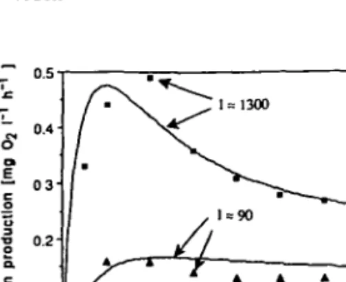
Harris and Piccinin (1977) investigated the photosynthetic behaviour of natural populations of phytoplankton. In some experiments samples collected from surface waters and kept in the dark for 5 min prior to the experiment were exposed to different light intensities. The oxygen production was monitored as a function of time. Figure 1 shows the result of one of these experiments. The data points are the experimental results derived from the original figure by Harris and Piccinin. The curves represent the corresponding simulations obtained with the model DYPHORA presented in the next section. The response of the cells to the light seems to be characterized by two time scales. First, there is an initial lag phase until the cells reach their full rate of photosynthesis. Second, on a longer time scale the effect of photoinhibition sets in for strong light. According to these experiments, the time for photosynthesis to reach a steady state varies between 15 and 60 min for different conditions.

Fig. 1. Comparison of simulation with DYPHORA (curves) with experimental data by Harris and

Piccinin (1977) (points). In the experiment mixed natural phytoplankton cultures previously kept in the dark for ~5 min were suddenly exposed to a constant light intensity /. Note that the scaling of the nondimensional P rates produced by the model relative to the absolute O2 production units

corresponds to the specific choice P^ = 1.8 mg O2 I"1 h~l (see equation 1). Model parameters:

T, = 20, Tr = 4, lcri, = 50, Ik = 790, K = 2 x 10"". See Table 1 for definitions and units of parameters.

Marra (1978a,b) performed a set of similar experiments using laboratory cultures. In his experiments it took a few hours of constant light intensities until steady state was achieved. The distinct difference in time scales between his experiments and the ones by Harris and Piccinin may be caused by the inequality of laboratory monocultures and natural populations; it may also reflect the variability in the dynamic response of different algal species.

In another type of laboratory experiment, Marra simulated typical light variations found in natural systems during a day. He observed that rates of photosynthesis in experiments where fluctuations were superimposed onto the daily light variation were larger than the rates for a 'regular' light curve with roughly the same mean intensity. This is additional evidence that light inhibition is a dynamic process.

More recent studies like those by Marra (1980), Falkowski (1980, 1983), Lewis and Smith (1983) and Post et al. (1984) showed that photoplankton exhibits a variety of different response reactions to light variation. Tentatively, we can distinguish two kinds of changes (Imboden, 1990): the reaction of cells due to light variations occurring over time scales between minutes and a few hours is called 'photoresponse'. The scales are of the same size as typical time scales of mixing (Denman and Gargett, 1983) and may thus be important for algal selection in different physical environments. In contrast, 'photoadaptation' is a process occurring on time scales of several hours to days. It involves structural changes in the state of the cell. An example for response would be the change in fluorescence or the change in size of the chloroplasts. An example for adaptation would be the change in the cellular composition, e.g. changes in chlorophyll (Platt and Gallegos, 1980).

The model named DYPHORA (DYnamic model for the PHOtosynthetic Rate of Algae) has first been suggested by one of the authors (D.M.I.) during a

Table I. Definition of variables of DYPHORA and their standard units Symbol t I V hri, / . - | ! _/ e for / s /m, ro for />/„,, Units min (j.E m~2 s"1 , E m -2s -M.E m-2 s-1 M.E m"2 s"1 b Definition Time Light intensity

Characteristic light intensity describing the equilibrium productivity curve Critical light intensity for onset of light inhibition

Inhibiting excess light intensity (Potential) rate of photosynthesis without photoinhibition

P b Actual rate of photosynthesis

P*q b Equilibrium P rate without inhibition

(equation 1)

Peq b Equilibrium P rate with inhibition

(equation 3)

Tr min Response time of P* for increasing /

i|i - Light inhibition function

4»e? — E q u i l i b r i u m inhibition function for

constant /

K (u,E m"2 s"1)"1 min"1 Inhibition growth constant

T,- min Inhibition decay time

°Ik is related to the equilibrium photosynthesis function proposed by Jassby and Platt (1976), Peq = Pmax tanh(a//Pmttt)//* = P^Ja.

b All rates of photosynthesis are expressed relative to the maximum equilibrium rate by Jassby and

Platt (1976), ?m, and are thus dimensionless (see equation 1).

workshop organized by the Centre of Limnological Modelling at the University of Western Australia in Nedlands/Perth. The aim of the model is to find the simplest mathematical formalism which is able to describe the dynamics observed in the P/I relationship. Thus, the approach is clearly empirical and not directed at the adequate description of the physiological and biochemical processes which are actually responsible for the complex behavior of the rate of photosynthesis. Ultimately, such an understanding is certainly needed, but we feel that the present experimental knowledge is still too scarce to expect a breakthrough. A similar approach has been used by Denman and Marra (1986). In their model the actual rate of photosynthesis is bounded by two PI I curves, one for dark-adapted and another for light-adapted algae. The degree of adaptation depends on the light history of the cell and is calculated with a linear response function.

Model description

The basic idea of the model DYPHORA lies in the dynamic response of the rate of photosynthesis P(t) to changing light intensities /(f). As a consequence, P does not simply depend on the actual light /—as it is the case in most existing models—but also on the prior light history. Obviously, every dynamic model also embraces a static model which can be derived by keeping the driving variable (/) constant long enough for the dependent variable (P) to reach an equilibrium (steady state), Peq. Although in nature steady state conditions

hardly ever occur, we first discuss the equilibrium properties of the model thus facilitating a comparison with existing static models.

The equilibrium PI I relationship consists of the noninhibited tanh function as suggested by Jassby and Platt (1976), and an equilibrium inhibition function tyeq (J). In order to simplify the discussion only relative rates will be computed. The

parameter Pmax by Jassby and Platt is used as a scaling factor:

P% (/) = "£*- = tanh (///*) (1)

where Pmaj:, Peq are the dimensional rates of photosynthesis (or of O2

production) and Pcq is the noninhibited, nondimensional rate. All variables and

their standard units are listed in Table I. The equilibrium inhibition function tyeq (/) is

-i^Kr, for l>Icrit &

where Icrit is the critical light for the onset of light inhibition. The meaning of the

(constant) parameters K and T, will become clearer when we discuss the dynamic properties of the model.

The inhibited equilibrium rate is defined as

p , n *% (0 t a n h TO j > j ( 3 )

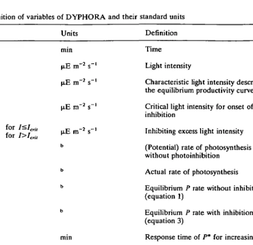
The functions P*q, i|/e<7 and Peq are shown in Figure 2a-c. Note from Figure 2c

that the maximum rate is significantly smaller than the maximum possible noninhibited rate (Figure 2a). This is due to the fact that the chosen parameter values obey Icri, < Ik meaning that light inhibition begins before the tanh function approaches its maximal value of 1. Indeed, it has been found in experiments that for light intensities ultimately leading to strong inhibition, the initial response of photosynthesis to the light is characterized by rates which are significantly higher than the maximal rate derived from the steady-state relationship Peq (I). An example by Harris and Piccinin (1977) was given in

Figure 1.

»,q(D=tanh(l/lk) _ £ 1 01 o c = 5 0.6 _ c_{m o}

0.4-H

l\ P(t) =

p*(t)

1+iMt)

Fig. 2. Illustration of model characteristics: (a-c) steady state values P*q, ty€q, and Peq as a function of light intensity/, and (d-f) temporal evolution of potential photosynthesis P* (no light inhibition), light inhibition function ty, and actual rate of photosynthesis Z3, if / is altered from 0 to / = 1000 at t =

0. Other model parameters: T, = 30, T, = 1, /,.„, = 250, Ik = 500, K = 1.3 x 10"4.

ways: first, it is postulated that for rising light intensity, /, the noninhibited rate of photosynthesis needs some time to get adjusted to the new light. The adjustment is described by the response time iy. In contrast, for decreasing /, the

P rate drops back to its lower value without time delay. Mathematically, this

- ^ - = -kr{P* - P*eq) (4a)

where

*' = C ' for??

p\ W

P* is the actual (potential) rate of photosynthesis if light inhibition did not exist.

Equation (4) expresses the fact that P* is always changing into the direction of the noninhibited rate P*q (equation 1) and that the downward adjustment occurs

instantaneously. The response of P* to light turned on from 0 to a constant value / = 1000 is shown in Figure 2d together with the analytical solution of equation (4) for this simple case.

The second dynamic effect is related to the inhibition function i|i by assuming that the effect of overcritical light is decaying with some time constant T,-. Thus, ty is described by the linear differential equation (see Table I for definitions)

(5) at

where the first term on the right-hand side describes the 'production' of inhibition, the second term the linear decay of accumulated inhibition. For constant / , 4> reaches a steady state (dtyfdt = 0) which is either 0 (/ ^ Icril) or

tyeq = {I ~ Icrit)TiK, in accordance with equation (2). For time-variable light, \\i(t)

is given by the convolution integral

\\i(t) = K f lex (f') exp dt' + i)»o e " ^ ' (6)

o

T,-where »|>o is the inhibition function at t = 0. In Figure 2e, ty (t) is plotted for a

sudden change of / from 0 to / = 1000 at t = 0. The analytical solution is of the same form as the solution of equation (4).

Having described the two dynamic elements we can now easily calculate the actual rate of photosynthesis, P(t), by the equation

The function is shown in Figure 2f for the example mentioned before. In response to the light, P{t) is first growing as P*. Later, the inhibition function (Figure 2e) becomes large enough to significantly depress P(t). Note that the dynamic behavior of P(t) is controlled by two intrinsic time scales, the response time for increasing light tr, and the inhibition decay time T,.

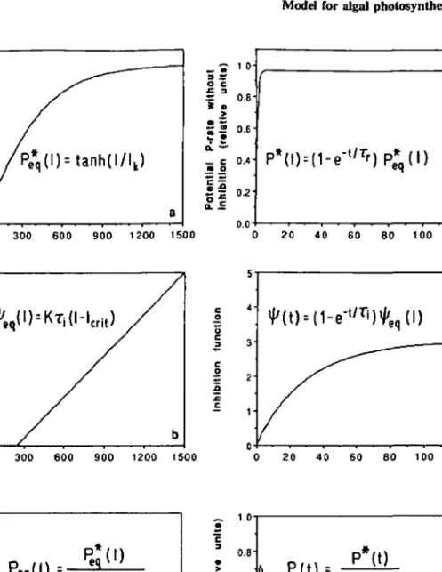
In Figure 3, calculations are presented which will demonstrate the influence of the several model parameters on the rate of photosynthesis. As for the preceding

•• 0.6-= 0.4-0 10.4-0 20.4-0 30.4-0 40.4-0 50.4-0 60.4-0 2 0.6-= 0.4 0 10 20 30 40 50 60 •> 0.6-= 0.4

Fig. 3. Sensitivity of DYPHORA with respect to various parameters demonstrated for a constant

light intensity / = 500 turned on at I = 0. Where not stated otherwise the following (default) values are used: T, = 30, T, = 1, / „ , = 250, Ik = 500, K = 1.3 x 10"". The P rates for the default parameter set are drawn as thick curves. Numbers indicate the value of the varied parameter, (a) Variation of response time T,; (b) variation of inhibition decay time T,; (C) variation of inhibition growth constant

examples, at t = 0 the light changes from zero to a constant value /. In each plot, the bold curve refers to the same set of parameters. In Figure 3a, the response time Tr is varied between 0.25 and 5 min. As indicated in Figure 2d, the increase of the potential (noninhibited) rate P* is controlled by the time scale -rr. Simultaneously, the inhibition function I|J grows as T,. Thus, the smaller the ratio Tr:T,, the larger is the maximum rate attained between the beginning of the experiment and the equilibrium value Peq. Note that Tr only influences the transient behavior of P(t) but leaves Peq unchanged.

In contrast, variation of T, affects the intermediate maximum of P{i) only slightly but directly determines Peq (equation 2). In Figure 3b, T, is varied

between 10 and 60 min. An intermediate case is met when K is altered (Figure 3c): the shape of the P(/) curve is influenced by K everywhere along the time axis.

Application of DYPHORA to laboratory measurements

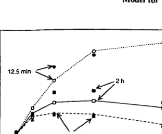
Marra (1978b) ran a comprehensive set of experiments with laboratory cultures of the alga Lauderia borealis. In the experiments the algae were grown at 12 h dark and light cycles under different constant light intensities. The oxygen production was monitored as a function of time t after the onset of the (constant) light period. Mean oxygen production rates were calculated for three different intervals T (12.5 min, 2 h, 4 h),

PT = ~

Wit) dt, (8)

I o

and plotted as a function of /.

A comparison of the original data and the result of the model simulation is shown in Figure 4. Compared with the parameter set used to explain the experiments by Harris and Piccinin (1977), the inhibition decay time T, needed to fit the experiments is significantly larger (120 instead of 30 min). Apparently, depending on the kind and preconditioning of the algae, widely different inhibition characteristics exist. In fact, the Pj{I) curve obtained from the short-time incubation shows no inhibition. The inhibition becomes apparent after 2 h incubation and still increases after 4 h. Note that the rates of mean photo-synthesis observed for the short incubation time are much higher than the maximum rates for the long term (quasi-steady state) mean values when the effect of photoinhibition has set in. Since for light intensities below about / = 300 the exposition time T has only little influence on PT, the critical intensity for

the onset of light inhibition (/„•,») must lie close to this value. The model simulations agree well with the experimental data for the 12.5 min and the 4 h incubation times, but they overestimate the effect of photoinhibition for the 2 h incubation time.

In another set of experiments the rate of oxygen production of laboratory cultures of L.borealis was monitored for the change in light intensity as occurring during a day (Marra 1978a). In the first experiment, the light followed

0.06

004

S 0 02

0 200 400 600 800 1000 1200 1400 Light Intensity [jiE m'V]

Fig. 4. Mean oxygen production rates PT as a function of light intensity / for three different averaging periods T = 12.5 min, 2 h, 4 h. Experimental data (open symbols) by Marra (1978b) from laboratory cultures of Lauderia borealis grown in 12 h dark-light cycles at different light intensities. Model calculations (closed symbols connected by lines) with T,- = 120, T, = 0.5, IcrU = 250, Ik = 825, K = 0.44 x 10~4. Absolute scaling of model result implies Pmax = 0.1 mol O2 h"1 cell"1.

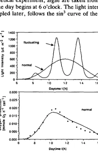
a simple sin3 curve, in the second experiment additional fluctuations in light intensity were superimposed such that the 12 h mean light intensities were roughly the same in both cases (Figure 5a).

In Figure 5b ,c the experimentally determined oxygen production rates are compared with model simulations using the same set of parameters as determined for the previous experiments (Figure 4). For the fluctuating light, experiment and model show an excellent agreement, especially with respect to the different peak rates during the two midday light maxima. Note that for both measurement and model, the afternoon maximum is significantly smaller than the morning peak. This is due to the long-term memory effect of the inhibition function I|I (f). A static (equilibrium) photosynthesis model cannot, of course, explain the asymmetry found in the experimental data.

For the 'normal' day (Figure 5b), the measured peak rate and the measured afternoon depression are both underestimated by the model. This phenomenon may be indicative of a second inhibition process governed by a larger time scale which is only triggered slowly and thus not important for the case of short-term light maxima (Figure 5c). Part of the extremely large T, value found here and in Figure 4 may be due to this second time scale. In fact, Neale and Marra (1985) have found two time scales—a short (<2 h) and a longer (5-6 h) scale in their experimental data. Long-term inhibition has also been observed in experiments conducted by Marra (1980) using laboratory cultures of Thalassiosira fluviatilis.

Significance of DYPHORA for field measurements of photosynthesis

There is doubtless enough experimental evidence to demonstrate the in-adequacy of a static PI I relationship. Though the few comparisons between experimental data and model calculations presented so far cannot serve as a

proof for DYPHORA in the strict mathematical sense, the model is nevertheless a suitable instrument to further explore the consequences of a dynamical P/I relationship. As an example let us address the following question:

Provided the dynamical model is correct, what kind of apparent static PI I relationship would a scientist derive from samples of algae taken from a lake and subsequently exposed to various light intensities in an incubator? Furthermore, what would be the discrepancies if two different methods were employed to measure photosynthesis, the measurement of O2 production (quasi-instan-taneous rate) and the 14C method (integrated rate)?

In our hypothetical experiment, algae are taken from the surface of a water body in which the day begins at 6 o'clock. The light intensity at the depth of the algae to be sampled later, follows the sin3 curve of the 'normal' day shown in

Fig. 5. Production rate P(l) during two different 'model days' of 12 h: 'normal' day has a sin3 light

regime, 'fluctuating' day has four light maxima and roughly the same mean light intensity as the normal day (plot a). Plots b and c: comparison of experiments by Marra (1978a) with laboratory cultures of Lauderia borealis (symbols) and model calculation (lines) for normal and fluctuating day, respectively. Model parameters as in Figure 4, scaling variable P^^, = 0.045 mol O2 h"1 cell"1.

Figure 5a and reaches its maximum of / = 1000 at noon. Samples are taken at two instants, at 10 and at 12 o'clock when the light intensity at the selected depth is 650 and 1000, respectively. Immediately afterwards the samples are put into incubators exposed to different (constant) light intensities.

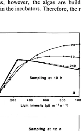
In the first type of experiment, photosynthesis is determined by O2 production after different incubation periods. In Figure 6 the mean rates calculated from DYPHORA are shown. The obtained Pll curves strongly depend on both the incubation and the sampling time. Samples taken at 10 h (Figure 6a) have not been exposed to overcritical light (/ > /„,, = 250) for too long. Thus, the 'preset' inhibition function i|/ is small so that at moderate incubator light intensities the measured rate does not change very much with incubation time t. For high light intensities, however, the algae are building up a significant inhibition while they are in the incubators. Therefore, the rates at a fixed / drop with incubation time.

_ 0.5

i -

0.3-0 20.3-0 0.3-0 40.3-00.3-0 60.3-00.3-0 S0.3-00.3-0 10.3-00.3-00.3-0 Light Intensity [nE m " : s ' ' ]

— 0.5

0.4-

0.3-200 400 600 800 1000 Light Intensity (ME m '2 S ' 1)

Fig. 6. Pseudo-static Pll curves derived from a hypothetical experiment using DYPHORA. Plankton is sampled at 10 h (plot a) and 12 h (plot b), respectively, and put into incubators at different light intensities /. Rates are determined after different incubation times (numbers are in minutes); they simulate instantaneous O2 production measurements. The true steady-state Pll relationship is drawn

for comparison (solid line). Model parameters are: T,- = 90, T, = 2, Icril = 250, lk = 825, K = 0.44 x 10~4. Previous light exposure as for the 'normal' day described in Figure 5.

In contrast, the samples taken at 12 h (Figure 6b) are strongly inhibited when they are put into the incubators. Thus, the PII curve measured after 20 min incubation time is strongly depressed compared with the curve measured for the samples taken at 10 h. Two hours after sampling, the P//curves look, however, alike for the two sampling times; the 'preset' inhibition function has lost most of its influence.

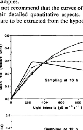
In the second kind of experiment, an integrated (mean) rate of photosynthesis is determined, thus simulating 14C experiments with different durations of incubation. For the samples taken at 10 h the precondition of the algae is of little influence. The main effect seen in Figure 7a originates from the inhibition in the incubator. Yet the samples taken at 12 h are already inhibited to such an extent that for all incubation times the mean production remains significantly smaller than in the other samples.

We certainly do not recommend that the curves of Figures 6 and 7 are taken for granted in their detailed quantitative aspects. However, the qualitative conclusions which are to be extracted from the hypothetical experiment cannot

0.5

= 0.4

=

0.3-£ 0.2

200 400 600 800 1000 Light Intensity [JIE m " * s ' ' ]

400 600 800 1000

Fig. 7. PII curves from the same type of hypothetical experiment as described in Figure 6, but with production rates determined as mean values over a given time interval as done for the '4C method.

Incubation begins immediately after sampling. The numbers indicate different durations of incubation. Model parameters as in Figure 6. Solid line: steady-state PII curve.

be ignored. They ask for caution with respect to the measurement of PI I relationships. Aside from the fact that such relationships do only apply to constant light conditions, we conclude that less bias is introduced if the equilibrium function Pe<?(7) shown in Figure 2c is determined by keeping the algae under constant light for several hours and then using the O2 method (instantaneous production rate). As can be seen from the true steady-state PI I curve, different types of error are introduced by the two methods. The O2 method measures the instantaneous rate. For both sampling times the true steady-state rate (rate reached after long exposure to constant light) is best represented after a long incubation time (240 min). For short incubation times, deviations from the true curve are either due to incomplete light inhibition for large / (Figure 6a) or due to 'preconditioned' inhibition at low / (Figure 6b).

In contrast, the 14C method represents an integrated rate. Though the difference between true and measured rates becomes smaller for increasing incubation time, the true rate is never reached since the integrated value always contains the effect of light adaptation or inhibition from the early part of the incubation period.

Discussion

The ability of DYPHORA to reproduce a variety of experimental data is taken as strong argument for the use of a model that relates the actual rate of photosynthesis to the light history of the cell rather than to the actual light intensity.

When formulating the model we did not intend to find mathematical expressions for specific physiological or biochemical processes. The physio-logical response of the cell results from the simultaneous action of different processes which are merely depicted by DYPHORA as an integrated response derived from experimental observation. In this respect, we consider DYPHORA to be just an intermediate tool which allows the exploration of the consequences of the dynamic PII relationship for the ecology of algae and for the interpretation of productivity measurements gained from plankton com-munities. The ultimate aim of this kind of research must lie in a full understanding of the biochemical and physiological aspects of photosynthesis and growth.

One important question requiring further investigations is related to the various time scales involved in photosynthesis. We have made a distinction between photoresponse and photoadaptation and thus tacitly assumed the existence of a 'spectral gap' between two kinds of adjustment processes. The model DYPHORA only addresses photoresponse; its time scales are thus limited to a few hours. But even within this range it seems that there are several superimposed processes which act on different time scales. Thus, DYPHORA with its two characteristic times (T,. and T,) may yield only an oversimplified picture of the 'true' situation.

In the mixed water column the cell may be exposed to extreme variations in light intensity within time intervals of minutes. The cell finds itself in the

dilemma of developing the right strategy to exploit the available energy and nutrient resources efficiently. If the efficiency of light harvesting is increased, then the sensitivity to damage caused by excess input of light quanta is simultaneously increased. An economical solution for the cell would be to develop a buffering capacity and a repair mechanism which operates on the time scale of the light fluctuations experienced. In contrast, a complete change of strategy, as may occur during photoadaptation, involves changes in cellular composition, the synthesis of chlorophyll, and in the number of photosynthetic units. Such an adaptation is quite energy demanding. In many cases changes asking for adaptation occur over longer time periods and are related to typical weather changes.

It is well known that algae in the field adapt to changing light conditions (Reynolds, 1984a; Falkowski, 1980). 'Shade algae' drawn from depth and characterized by a high pigment content and high photosynthetic efficiency are liable to rapid photoinhibition. Algae grown in well-isolated epilimnia of stratified lakes have smaller photosynthetic efficiencies but are less susceptible to photoinhibition. Adaptive changes are also observed on a daily base as a consequence of the variability in the environment and in community structure (Cote and Platt, 1983). In this respect the question arises of whether algae adapted to different light regimes are not only different in their steady-state characteristics but also in their dynamic response to rapidly changing light.

Reynolds (1984a,b) has studied the succession of algae in lakes and has grouped the species into several classes depending on the difference in adaptive strategies for effectively exploiting alternative environments. The changes in light availability seem to be one of the major selection criteria for some species to dominate. It can be expected that the light response for those species which perform well under mixing conditions is characterized by the following features: (i) The response time jr must be fast relative to the typical time scale of light

variation, (ii) The absorption spectrum of the light-harvesting pigments should cover a broad range of wavelengths due to the changing spectral composition of light within the water column (Jeffrey, 1980). (iii) The ability to exploit a broad range of light intensities and wavelengths should result in a relatively low efficiency and hence in a low maximal rate compared with species being adapted to a defined light environment. Based on these assumptions we are currently investigating the possible difference in the photoresponse function for species dominating under stratified and mixed conditions, respectively. Yet, the response to light is only one of several factors. For a species to dominate, the actual growth rate which depends on nutrient availability and all loss processes, must be higher than the growth rate of the competing species. Therefore, the results from short-term experiments must be complemented by long-term experiments.

The prediction of a critical patch size based on the interplay of horizontal diffusion and algal growth has been one of the first examples to relate physical and biological scales (Kierstead and Slobodkin, 1953; Skellam, 1951). This work has triggered many further investigations in this direction (Okubo, 1980). The intention of this article is to promote and encourage experimental investigations

addressing yet another aspect of the coupling between physical and biological processes. Such data may help to interpret the enormous amount of information on algal growth and to gain further insight into the factors governing aquatic ecosystems.

References

C6te,B. and Platt.T. (1983) Day-to-day variations in the spring-summer photosynthetic parameters of coastal marine phytoplankton. Limnol. Oceanogr., 28, 320-344.

Denman.K.L. and Gargett,A.E. (1983) Time and space scales of vertical mixing and advection of phytoplankton in the upper ocean. Limnol. Oceanogr., 28, 801-815.

Denman.K.L. and Marra,J. (1986) Modelling the time dependent photoadaptation of phytoplank-ton to fluctuating light. In Nihoul.L.C. (ed.), Marine Interfaces Ecohydrodynamics, Elsevier Oceanography Series, No. 42.

Falkowski.P.G. (1980) Light-shade adaptation in marine phytoplankton. In Falkowski.P.G. (ed.), Primary Productivity in the Sea, Plenum Press, New York, pp. 99-119.

Falkowski,P.G. (1983) Light-shade adaptation and vertical mixing of marine phytoplankton: a comparative field study. /. Mar. Res., 41, 215-237.

Harris,G.P. and Picrinin,B.B. (1977) Photosynthesis by natural phytoplankton populations. Arch. Hydrobiol., 80, 405-456.

Imboden.D.M. (1990) Mixing and transport in lakes: Mechanisms and ecological relevance. In Tilzer,M. and Serruya.C. (eds), Large Lakes: Ecological Structures and Functions. Springer, Berlin, pp. 47-80.

Jassby,A.D. and Platt.T. (1976) Mathematical formulation of the relationship between photosyn-thesis and light for phytoplankton. Limnol. Oceanogr., 21, 540-547.

Jeffrey,S.W. (1980) Algal pigment systems. In Falkowski.P.G. (ed.), Primary Productivity in the Sea, Plenum Press, pp. 33-58.

Kierstead,H. and Slobodkin,L.B. (1953) The size of water masses containing plankton blooms. J. Mar. Res., 12, 141-147.

Lewis.M.R. and Smith,J.C. (1983) A small volume, short-incubation-time method for measurement of photosynthesis as a function of incident irradiance. Mar. Ecol. Prog. Ser., 13, 99-102. Marra,J. (1978a) Effect of short-term variations in light intensity on photosynthesis of a marine

phytoplankter: a laboratory simulation study. Mar. Bioi, 46, 191-202.

Marra.J. (1978b) Phytoplankton photosynthesis response to vertical movement in a mixed layer. Mar. Biol., 46, 203-208.

Marra.J. (1980) Vertical mixing and primary production. In Falkowski,P.G. (ed.), Primary Productivity in the Sea, Plenum Press, pp. 121-137.

Neale,P.J. and Marra.J. (1985) Short-term variation of /*„,„ under natural irradiance conditions: a model and its implications. Mar. Ecol. Prog. Ser., 26, 113-124.

Okuba.A. (1980) Diffusion and Ecological Problems: Mathematical Models. Springer-Verlag, Berlin.

Platt.T., Gallegos.C.L. (1980) Modelling Primary Production. In Falkowski,P.G. (ed.), Primary Productivity in the Sea, Plenum Press, pp. 339-362.

Post.A.F., Dubinsky.Z., Wyman.K. and Falkowski.P.G. (1984) Kinetics of light-intensity adapt-ation in a marine planktonic diatom. Mar. Biol., 83, 231-238.

Reynolds.C.S. (1984a) The Ecology of Freshwater Phytoplankton. Cambridge University Press, Cambridge.

Reynolds.C.S. (1984b) Phytoplankton periodicity: the interaction of form, function and environ-mental variability. Freshwat. Biol., 14, 11-142.

Skellam.J.G. (1951) Random dispersal in theoretical populations. Biometrika, 78, 196-218. Received on September 5, 1989; accepted on June 25, 1990