Rcrust: a tool for calculating path-dependent open system processes and application to melt loss

(1)

by

Matthew Jason Mayne

Thesis presented in fulfilment of the requirements for the degree of Master of Science in the Faculty of Science at Stellenbosch University

Supervisor: Prof. Gary Stevens, Stellenbosch University

Co-supervisor: Prof Jean-François Moyen, Université de Saint-Etienne (France)

(2)

Declaration

By submitting this thesis electronically, I declare that the entirety of the work contained therein is my own, original work, that I am the sole author thereof (save to the extent explicitly otherwise stated), that reproduction and publication thereof by Stellenbosch University will not infringe any third party rights and that I have not previously in its entirety or in part submitted it for obtaining any qualification.

March 2016

(3)

iii

ABSTRACT

Earth‘s continental crust is stabilised by crustal differentiation that is driven by partial melting and melt loss: Magmas segregate from their residuum and migrate into the upper crust, leaving the deep crust refractory. Thus, compositional change is an integral part of the metamorphic evolution of anatectic granulites. Current thermodynamic modelling

techniques have limited abilities to handle changing bulk composition. New software is developed (Rcrust) that via a path-dependent iteration approach enables pressure,

temperature and bulk composition to act as simultaneous variables. Path-dependence allows phase additions or extractions that will alter the effective bulk composition of the system. This new methodology leads to a host of additional investigative tools. Singular paths within Pressure-Temperature-Bulk composition (P-T-X) space give details of changing phase proportions and compositions during the anatectic process, while compilations of paths create path-dependent P-T mode diagrams. A case study is used to investigate the effects of melt loss in an open system for a pelite starting bulk composition. The study is expanded upon by considering multiple P-T paths and considering the effects of a lower melt threshold. It is found that, for the pelite starting composition under investigation, open systems produce less melt than closed systems and that melt loss prior to decompression drastically reduces the ability of the system to from melt upon decompression.

(4)

iv

OPSOMMING

Korsdifferensiasie stabiliseer die kontinentale kors van die aarde tydens gedeeltelike smelting. Magma segregeer van hul residuum en migreer in die vlakker kors in. As gevolg daarvan raak die diepkors meer vuurvas. Dus speel komposisionele verandering ‗n belangrike rol in die evolusie van anatektiese granuliete. Hedendaagse termodinamiese modelleringstegnieke het beperkte vermoëns om 'n veranderende grootmaatsamestelling te hanteer. Nuwe sagteware is ontwikkel (Rcrust) wat 'n roete-afhanklike iterasie benadering volg. Hierdie metode laat die druk, temperatuur en grootmaatsamestelling toe om as gelyktydige veranderlikes te funksioneer. Roete-afhanklikheid laat fasetoevoegings of ekstraksies toe om die effektiewe grootmaatsamestelling van die stelsel te verander. Die nuwe metode bied ‗n magdom verskeie maniere aan om ondersoek in te stel. Enkel roetes van P-T-X ruimte beskryf die fase proporsies en komposisies tydens die proses anatektiese, terwyl kombinasies van roetes, roete-akhanklike pseudosections skep. 'n Gevallestudie is op uitgebrei om die gevolge van smeltverlies te ondersoek. Dit is bevind dat oop stelsels minder produktief by smelt vorming is as geslote stelsels, en dat dekompressie smelt minder produktief as verwarming is. Die verlies in smelt produktiwiteit van die oop stelsel impliseer beperkings op die maksimum massa dekompressie smelt wat kan vorm. Tektoniese modelle wat dekompressie smelt as bron van groot volumes smelt gebruik moet dus herevalueer word.

Sleutelwoorde: Rcrust, Anatekse, smeltverlies, termodinamiese modellering, dekompressie smelt

(5)

v

ACKNOWLEDGEMENTS

Funding by the South African National Research Foundation (NRF) through the Scare Skills Bursary to M.J. Mayne and from the South African Research Chairs Initiative (SARChl) to G. Stevens is gratefully acknowledged. M.J. Mayne would like to acknowledge support from the European Research Council (project MASE, ERC StG 279828 to J. van Hunen).

I would like to thank my supervisors Prof. Gary Stevens and Prof. Jeff Moyen for their constant attention and assistance throughout the project. In addition, I would like to thank my family and friends for their support and patience. This work was orally presented by M.J. Mayne at the Granulites & granulites conference, 2015 in Windhoek, Namibia.

(6)

vi

LIST OF FIGURES

Fig. 1 Flow chart of the Rcrust program structure

Fig. 2 Drop down based Rcrust GUI

Fig. 3 Flow chart of the magma extraction algorithm

Fig. 4 Rcrust P-T psuedosection with phase proportion paths for the isobaric heating path at 12 kbar (IBH12)

Fig. 5 Rcrust clockwise P-T path and phase mode diagrams

Fig. 6 Contour plots of biotite, muscovite and total melt in the full system for the closed system case as well as path-dependent

P-T mode diagram for a compilation of isobaric heating

paths

Fig. 7 Contour plots for 7 vol.% threshold path-dependent P-T mode diagrams showing interstitial melt, total melt and H2O

in the residuum for the isobaric heating system and the 12kbar isobaric heating followed by isothermal

decompression system

Fig. 8 Phase boundaries and garnet-biotite mode difference for the 7 vol.% threshold 12kbar isobaric heating followed by isothermal decompression system

Fig. 9 Contour plots for 1 vol.% threshold path-dependent P-T mode diagrams showing interstitial melt, total melt and H2O

in the residuum for the isobaric heating system and the 12kbar isobaric heating followed by isothermal

decompression system Page 8 10 11 15 18 20 24 26 29

(9)

ix Fig. 10 Melt productivity difference (MPD) contours for 1 vol.%

threshold path-dependent P-T mode diagrams

SUPPLEMENTARY FIGURES

Sup Fig. 1 Contour plots for P-T modes in the closed system

Sup Fig. 2 Contour plots for path-dependent P-T modes in the 7 vol.% threshold isobaric heating system

Sup Fig. 3 Contour plots for path-dependent P-T modes in the 7 vol.% threshold 12kbar isobaric heating followed by isothermal decompression system

Sup Fig. 4 Contour plots for path-dependent P-T modes in the 1 vol.% threshold isobaric heating system

Sup Fig. 5 Contour plots for path-dependent P-T modes in the 1 vol.% threshold 12kbar isobaric heating followed by isothermal decompression system

Page 31 43 44 45 46 47

(10)

x

LIST OF TABLES

Table 1 Starting bulk composition used in the construction of pseudosections

Page

(11)

xi

LIST OF ABBREVIATIONS

Minerals:

Abbreviations for rock forming minerals were taken from Whitney & Evans (2010) as:

And Andalusite Bt Biotite Cpx Clinopyroxene Crd Cordierite Grt Garnet H2O Water Ilm Ilmenite Kfs Alkali feldspar Ky Kyanite Liq Liquid Mag Magnetite Ms Muscovite Opx Orthopyroxene Pl Plagioclase feldspar Qz Quartz Sil Sillimanite Spl Spinel

(12)

xii Terminology:

AS Addition subsystem

ES Extract subsystem

FS Full system

ΔG Change in Gibbs free energy of the system

GUI Graphical user interface

IBH Isobaric heating

IBH12 Isobaric heating at 12 kbar pressure

ITD Isothermal decompression

MCT Melt Connectivity Transition

ML Melt loss event

mol.% molar percentage

mol*,% one oxide normalised molar percentage

NCKFMASHTO Na2O-CaO-K2O-FeO-MgO-Al2O3-SiO2-H2O-TiO2-O

PAE Peritectic assemblage entrainment

P-T-X Pressure-Temperature-Bulk composition

RS Reactive subsystem

TCL Tool Command Language

vol.% volume percentage

(13)

1

CHAPTER 1 CONTRIBUTIONS OF THE AUTHORS

Professor Jean-François Moyen along with Professor Vojtěch Janoušek created the first form of Rcrust using a phase stability calculation routine that called meemum from the Perple_X suite of programs as an executable. I was introduced to the program and the R coding language by Professor Moyen after which I took over further development of Rcrust.

I wrote a new phase stability calculation routine which uses a wrapper (compiled by Dr Lars Kaislaniemi) to perform calculations directly in the global environment making it quicker and more robust. I created save and load routines whereby simulation parameters are communicated through a text document. I developed initialisation routines for starting variables and severed the need for an initial meemum build file. I then created a graphical user interface to allow ease of use. I introduced the idea of a full system which is split into addition; extraction and reactive subsystems with routines that pass phases between them. I created some rudimentary output routines including a colour map using identification numbers of unique phase assemblages encountered by points along a path.

To investigate the uses of Rcrust, I performed a case study which reproduced the results of Yakymchuck & Brown (2014) but without using the manual stitching together of pseudosections. I expanded this case study by compiling P-T-X paths into a new type of diagram we call path-dependent P-T mode diagrams which I used to investigate the effects of melt loss on the total melt productivity of open systems (Chapter 2: Presentation of the research paper). I then developed these results into a manuscript which was submitted to the Journal of Metamorphic Geology. Throughout the coding and writing processes Professor Gary Stevens and Professor Jean-François Moyen provided academic guidance. Dr Lars Kaislaniemi compiled the Perple_X wrapper and provided insightful comments on the final manuscript.

REFERENCES

Yakymchuk, C. & Brown, M., 2014. Consequences of open-system melting in tectonics. Journal of the Geological Society, 171, 21-40.

(14)

2

CHAPTER 2

(15)

3

Rcrust: a tool for calculating path-dependent open system

processes and application to melt loss

M. J. MAYNE1 , 2 ,*, J.-F. MO YEN2, G. STEVENS1, L. KAIS LANIE MI3 1 Center for Crustal Petrology, Department of Earth Sciences, Stellenbosch University, Private Bag X1, Matieland 7602, South Africa

2 Université Jean Monnet, 23 Rue du Docteur Paul Michelin, 42023 Saint-Etienne, Cedex 2, France

3 Institute of Seismology, Department of Geosciences and Geography, University of Helsinki. Gustaf Hällströmin katu 2b, 00014 Helsinki, Finland

* corresponding author ([email protected])

(16)

4 ABSTRACT

Earth‘s continental crust is stabilised by crustal differentiation that is driven by partial melting and melt loss: Magmas segregate from their residuum and migrate into the upper crust, leaving the deep crust refractory. Thus, compositional change is an integral part of the metamorphic evolution of anatectic granulites. Current thermodynamic modelling

techniques have limited abilities to handle changing bulk composition. New software is developed (Rcrust) that via a path-dependent iteration approach enables pressure,

temperature and bulk composition to act as simultaneous variables. Path-dependence allows phase additions or extractions that will alter the effective bulk composition of the system. This new methodology leads to a host of additional investigative tools. Singular paths within Pressure-Temperature-Bulk composition (P-T-X) space give details of changing phase proportions and compositions during the anatectic process, while compilations of paths create path-dependent P-T mode diagrams. A case study is used to investigate the effects of melt loss in an open system for a pelite starting bulk composition. The study is expanded upon by considering multiple P-T paths and considering the effects of a lower melt threshold. It is found that, for the pelite starting composition under investigation, open systems produce less melt than closed systems and that melt loss prior to decompression drastically reduces the ability of the system to from melt upon decompression.

(17)

5 1. INTRODUCTION

Crustal differentiation occurs by partial melting of deep crust at high temperatures (Clemens, 1984; Scaillet et al., 1998), segregation of an incompatible element enriched magma from a more refractory residuum (Clemens & Stevens, 2012) and the migration of the magma to a higher crustal level (Clemens, 1990). Magmas may entrain crystals from the source (Stevens

et al., 2007; Villaros et al., 2009; Taylor & Stevens, 2010) and may further evolve through

segregation of crystals from melt as the magma ascends and cools (Johnson et al., 2015; Morfin et al., 2014; Sawyer, 2001; Sawyer, 1996). Throughout these processes bulk compositional change of the source and magma is fundamental to crustal differentiation.

Effective bulk composition of the source and of the magma can change throughout the anatectic process by multiple mechanisms. Magma segregation separates the bulk composition into portions that may evolve separately. Varying proportions of peritectic assemblage entrainment (PAE) to the magma influences the bulk compositions of the separated portions (Stevens et al., 2007; Clemens & Stevens, 2012). Kinetic effects can limit the availability of a phase to the system, for example, the slow diffusion of species in plagioclase (Morse, 1984) or garnet (Zuluaga et al., 2005; Taylor & Stevens, 2010) forcing dissolution to be the rate limiting factor or alternatively entire portions of phases can be isolated from reactions by their inclusion in other phases. Thus the effective bulk composition of the system is dependent on the P-T path. Compositional changes of magma and residuum have important implications for further melt production. A recent paper by Yakymchuck & Brown (2014) has criticised the inference of large amounts of decompression melt production across hydrate breakdown reactions. They argued that compositional changes invoked by melt loss on prograde segments of clockwise P-T paths would reduce the ability of the rock to form melt upon suprasolidus decompression. They suggested that large melt volumes, rather than being the result of decompression melting, could be the result of suprasolidus melt transfer and accumulation at shallow levels. Consequently it is crucial for studies of the partial melting of the crust to investigate the combination of pressure (P), temperature (T) and bulk compositional (X) effects.

1.1. Thermodynamic modelling tools

Phase equilibria modelling has contributed enormously to our understanding of the process of anatexis in crustal rocks (White & Powell, 2002; Johnson et al., 2008; White et al., 2007).

(18)

6 Phase equilibria were originally displayed on petrogenetic grids (Albee, 1965). Compositionally relevant phase diagrams were created from these grids by considering a single bulk composition thereby creating pseudosections of P-T-X space (Hensen & Essene, 1971; Hensen & Harley, 1990). The compilation of internally consistent thermodynamic datasets allowed the quantitative calculation of subsolidus phase equilibria (Helgeson et al., 1978; Powell & Holland, 1985; Powell & Holland, 1988; Gottschalk, 1997; Holland & Powell, 1998). Computer programs have been used to create pseudosections by either using the simultaneous solution of non-linear equations as is the case in THERMOCALC (Powell & Holland, 1988; Powell et al., 1998) or the minimisation of Gibbs free energy of the system (ΔG) as is the case in Perple_X (Connolly & Kerrick, 1987) and Theriak/Domino (de Capitani & Petrakakis, 2010). Increased usage of pseudosections in metamorphic studies created a demand for more accurate and applicable solution models which have become more sophisticated with time. The development of solution models for melt (Berman & Brown, 1984; Ghiorso & Sack, 1995; Holland & Powell, 2001; White et al., 2001) allowed thermodynamic modelling to begin to consider partial melting processes.

The behaviour of natural anatectic systems mandates investigations to consider a changing bulk composition. Current software manages a changing bulk composition by setting pressure or temperature constant then scaling between two end members via T-X or P-X sections. This is achieved by using the fractionation abilities of Perple_X or Theriak/Domino (Connolly, 2005; de Capitani & Petrakakis, 2010); by using the ‗read bulk info‘ script from THERMOCALC (Powell et al., 1998) or by manually ‗stitching together‘ different pseudosections each time the bulk composition changes (White & Powell, 2002; Brown & Korhonen, 2009, Yakymchuck & Brown, 2014).

1.2 Modelling compositional change in P-T-X space

Examples of studies investigating compositional change include: water content (e.g. White & Powell, 2002; Johnson et al., 2003; Diener et al., 2008; Johnson et al., 2010; White & Powell, 2010), amount of melt lost from the system (e.g. White & Powell, 2002; Johnson et al., 2003; Johnson et al., 2008; Brown & Korhonen, 2009; Korhonen et al., 2010) or molar proportion of an elemental oxide (e.g. Johnson et al., 2008; Johnson et al., 2010).

Diagrams that require bulk compositional change beyond the capabilities of a binary compositional range are generally created as stitched panels where each panel is a separately calculated pseudosection. An example of this is X scaled as melt loss with separate

(19)

7 panels for each melt loss event (e.g. White & Powell, 2002; Brown & Korhonen, 2009). Phase proportions can be investigated with T-X or P-X diagrams where X is the proportion of the phases (e.g. Johnson & Brown, 2011; Johnson et al., 2010; Johnson et al., 2008; de Capitani & Petrakakis, 2010; White & Powell, 2010; Yakymchuck & Brown, 2014). Advances in software have allowed pressure to vary within a T-X diagram or temperature to vary within a P-X diagram by allowing the user to make one variable dependent on the other thus simulating a P-T path (Connolly, 2005; de Capitani & Petrakakis, 2010).

Graphing compositional change by manually stitching panels becomes prohibitively time consuming when investigating multiple melt loss events or when investigating a variety of bulk compositional controls. This limits the resolution of studies that consider bulk compositional change. The aim of this paper is to introduce a new phase equilibrium modelling tool where pressure, temperature and bulk composition can change simultaneously with an automated handling of bulk compositional change. This paper presents the program‘s functionalities and the petrological constraints that it operates within. Explanations relating to the code are kept to a minimum with any important coding variables presented in italics. A case study is performed to demonstrate the capabilities of the program and highlight the ways in which it can provide added functionality in the study of anatectic systems.

2. RCRUST: A PATH-DEPENDENT APPROACH

In this study new software has been developed to provide a functional and efficient tool for investigating crustal anatexis. The software is named ‗Rcrust‘ to emphasise its applicability to crustal anatectic simulations and identify R (Ihaka & Gentleman, 1996) as its coding language. Rcrust operates by calculating the stable phases for a number of points in P-T-X space. For each starting bulk composition chosen a user defined P-T path can be explored.

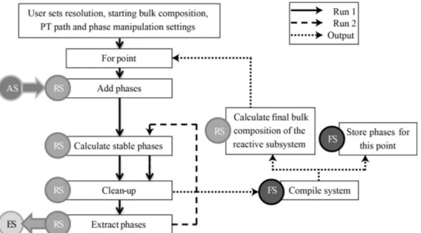
At each point along this path Rcrust defines the full system (FS) that consists of a reactive subsystem (RS) which is in chemical equilibrium with the P-T-X conditions of the point, an extract subsystem (ES) where phase extractions are stored and an addition subsystem (AS) where phases not yet incorporated in the reactive system are stored (Fig. 1). The extract and addition subsystems are not necessarily in chemical equilibrium with each other, the reactive subsystem or the given P-T-X conditions of the point. Phase extractions and additions, can be performed on the reactive subsystem at set points on the path or

(20)

8 triggered by set criteria met by the reactive subsystem (for example phase abundances in the reactive subsystem can be used to trigger events when a melt threshold is exceeded).

These manipulations (additions or extractions) alter the bulk composition of the reactive subsystem. The final composition of the reactive subsystem at the end of each point‘s phase manipulations is used as the starting composition of the next point on the path. Points along a path are considered sequentially therefore criteria met in the beginning of a path determine the conditions met by points later in the path. Thus, each point in the P-T-X path calculated is path-dependent. Any number of phase manipulations can occur at each P-T-X point allowing pressure, temperature and all n compositional variables of the bulk composition in an n-component system to vary simultaneously. The resolution (number of points) can be increased to make the P-T-X change between each point small enough that a continuous process is effectively mapped.

Stable phases are calculated by calling a compiled form of the meemum function from the Perple_X suite of programs (Connolly & Kerrick, 1987; Connolly, 2005; Connolly, 2009). This function, given the pressure, temperature and bulk composition of the system, will return the stable mineral phases and their compositions via Gibb‘s free energy minimisation of the system (ΔG) (Connolly & Kerrick, 1987; Connolly, 2005; Connolly, 2009). The P-T-X conditions for each point in Rcrust are passed through the function and the outputs are recorded. Bulk compositional manipulations are performed in Rcrust by a series of functions as defined below. The modular form of the functions allows them to be added or changed without affecting the integrity of the overall program.

Fig. 1 - Flow chart illustrating the Rcrust program structure for a single simple path. The user inputs the

calculation‘s resolution, starting bulk composition, P-T path and phase manipulation settings. Each step in a simulation consists of two runs and an output. The first run is shown in a solid line, the second run in a dashed line and the outputs in a dotted line. Grey circles show the system or subsystem involved in each step as AS (addition subsystem), ES (extract subsystem), FS (full system) or RS (reactive subsystem). Arrows show interactions between systems.

(21)

9 2.1 How it works

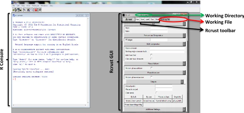
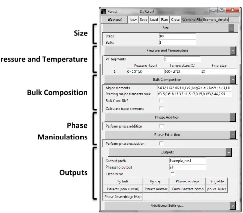
The user inputs parameters into an interactive Graphical User Interface (GUI) including initial bulk compositions, P-T paths, thermodynamic dataset, solution models and phase manipulation settings (Fig. 2). The current GUI only has basic functions but will be expanded with future development. P-T paths can be defined by individual points or by a series of functions, allowing consideration of complex P-T paths.

For the first calculable point the starting bulk composition is initialised as the reactive subsystem and used to calculate the stable phases under the given P-T-X conditions. If no phase manipulations are required at that point then the stable phases will be cleaned up and compiled into a system which records each point‘s phase compositions, proportions and additional properties. The clean-up process uses abundance and density values from the phase stability calculation to determine the mass and volume of phases. In addition phases‘ names, that are duplicated due to the presence of solvi in particular solution models (e.g. spinel, feldspar, etc.), are numbered for ease of identification. For convenience any feldspar with more K2O than CaO (in wt.%) is labelled as ―Kf‖.

Points can undergo phase manipulations consisting of ‗phase additions‘- phases that are added into the reactive subsystem and ‗phase extractions‘ – phases that are removed from the reactive subsystem. Phase additions are incorporated into the reactive subsystem in the first run of a point so that criteria set on the system take into account the new phase additions (Fig. 1 solid line). Phase extractions operate on the second run of a point so that newly re-equilibrated phase additions can form part of the (extractable) reactive subsystem (Fig. 1 dashed line).

Phase additions and extractions can be invoked at predefined points in the P-T path (by point) or when set criteria in the system are met (by condition). These conditions can involve any composition, proportion or property of the stable phases. For example, extraction can be set to occur whenever a specified value is exceeded (threshold), such as melt extraction occurring whenever a specified melt proportion is exceeded. Conditions on phase proportions can be given as a weight (wt.%), molar (mol.%) or volume (vol.%) percentages. When phase addition or extraction events are triggered the operations are performed on a mass basis. Alternatively phase extractions can extract a percentage value of the phase present. Outputs from the end of the second run are cleaned up and stored with letters indicating the subsystem it forms part of as either addition subsystem (AS), extract subsystem (ES) or reactive subsystem (RS). Runs are performed sequentially and outputs recorded for the number of points specified by the user.

(22)

10 Fig. 2 - Drop down based Rcrust GUI created using the cross-platform (Tcl/Tk) widget toolkit from Ousterhout

(1993).

2.2. Custom functions - magma extraction

Phase manipulations can be utilised in their generic forms or customised to suit a petrological problem. For example, as magma extraction from the source is a key aspect of crustal differentiation a custom phase extraction function was set up to model this process (Fig. 3).

The Extract Magma function has the same ability to extract by condition or by

point as the standard phase extraction function. The by condition argument allows magma

extraction to occur whenever a melt threshold is met (the point at which this happens does not need to be known before extraction). Natural magma extraction may leave behind a small amount of melt on grain boundaries (Sawyer, 2001; Marchildon & Brown, 2002; Holness & Sawyer, 2008). Accordingly Retention mode enables melt extraction until a set proportion of melt is left (this approximates the melt retention amount). In this study the Extract Magma function is used only to extract melt but future studies could consider extracting melt along with crystals (this functionality is currently available in Rcrust). This could be useful to investigate, for example, the entrainment of peritectic phases in a magma.

(23)

11 Fig. 3 - Flow chart of the magma extraction algorithm. Grey hexagon shaped boxes are decision points. Coding

variables are in italics. The For phase loop (dotted line) is repeated until each phase tagged for extraction has been considered. If ‗Retention mode‘ is active melt is considered last so that other phases extracted are accounted for in its calculation.

2.3. Outputs

Data from Rcrust can be analysed directly in R, written to file (in text format) or accessed by any R compatible package. One such package, only available for Microsoft Windows®, is Geochemical Data Toolkit (GCDkit). GCDkit is a free package in R that allows plotting of graphical outputs and enables users without a programming knowledge to utilise R‘s statistical functions (Janoušek et al., 2006).

3. PROGRAM DESCRIPTION

3.1. Thermodynamic calculations

Thermodynamic calculations are performed by a compiled form of the meemum function from the Perple_X suite of programs (Connolly & Kerrick, 1987; Connolly, 2005; Connolly,

(24)

12 2009). This is freely available allowing the inclusion of the necessary components in Rcrust‘s program files, which ensures compatibility across versions and sets the installation options which could otherwise be a source of user error.

3.2. Code manipulations

The program‘s code is written in R version 2.13.2 (2011-09-30) of R. Copyright © 2011 the R Foundation for Statistical Computing. R is an object-oriented statistical language built to combine the strengths of two other languages: S by Becker et al. (1988); and Scheme by Steele & Sussman (1975). This software is open-sourced and requires a machine with at least 32-bit addresses and 2 or more megabytes of directly accessible memory (Ihaka & Gentleman, 1996). R functions on a variety of UNIX platforms, Windows and MacOS.

Calculations in R require no fixed data structures, allow missing values (as ‗not applicable‘ or ‗not a number‘ replies) and follow powerful high level structures. Included in R are multiple arithmetic, statistical and database functions. A limitation of R is that data is stored internally; therefore a system crash results in the loss of the current environment (Ihaka & Gentleman, 1996). Further problems arise in R‘s complex syntax and non-user-friendly console. The geologist‘s psychological barrier to programming and the steep learning curve to new programming languages suggest that for a modelling tool to be applied successfully to address problems in the geosciences, it must minimise the interaction between the user and the underlying code. For this purpose a Graphical User Interface (GUI) was constructed.

3.3. User interface

Tool Command Language (TCL) is an embedded command language created by Ousterhout (1993). This language enables a cross-platform widget toolkit (Tcl/Tk) that provides a number of widgets needed to build GUIs. The Tcl/Tk package version 2.13.2 was chosen for the development of the Rcrust GUI for its cross platform capabilities and free format. The current version of the Rcrust GUI however is only stable in the Windows environment. The Tcl/Tk package is included within the Rcrust install files so does not require separate installation from the user. Further, this ensures compatibility between the version of package in which the GUI is both written and displayed.

(25)

13 4. CASE STUDY

In order to assess the validity of Rcrust‘s calculation routines and the applicability of the program to geological scenarios a case study is performed based on a recent paper (―Consequences of open-system melting in tectonics‖) by Yakymchuck & Brown (2014). This paper was chosen as it highlights the use of ‗pseudosection stitching‘ to model open system processes.

4.1. Model set up by Yakymchuck & Brown (2014)

Yakymchuck & Brown (2014) used a series of P-T pseudosections for bulk chemical compositions modified by a sequence of melt loss events to investigate open-system melting behaviour. The system was set to be conditionally open by extracting melt from the system whenever a melt threshold was exceeded. They modelled two bulk compositions, but for reasons of space here we only investigate the average amphibolite-facies pelite composition that they considered from Ague (1991) (Table 1). Their calculations were performed in THERMOCALC version 3.35 (Powell & Holland, 1988) using the internally consistent dataset of Holland & Powell (1998) in the NCKFMASHTO (Na2O-CaO-K2

O-FeO-MgO-Al2O3-SiO2-H2O-TiO2-O) chemical system. The activity-composition (a-x) models they used

are stated in Yakymchuck & Brown (2014).

They set the H2O content of the bulk composition to allow the system to be fully

hydrated but with only a small proportion of free fluid (<0.1 mol*.% free H2O; phase

proportions calculated with THERMOCALC output mol.% normalised to a one oxide basis so are referred to in this paper as mol*.%) just below the solidus (at 12 kbar). This was done to ensure fluid-absent melting conditions. These normalised mol*.% values approximate volume proportions.

Yakymchuck & Brown (2014) defined melt loss in the open system to occur when an interconnected melt network forms and the matrix compacts. This was considered to happen when >80% of grain boundaries become melt bearing at the rheological transition defined by the Melt Connectivity Transition (MCT) of 7 vol.% melt, the upper limit of the accumulation of melt before extraction (Rosenberg & Handy, 2005). Melt retention on grain boundaries was estimated to be 1 vol.% (Yakymchuck & Brown, 2014). They assumed both of these vol.% constraints to be approximated by equivalent one oxide normalised mol*.%.

(26)

14 Calculations were performed in a P-T area from 2-12 kbar and 640-920 °C (Fig. 4a). In the closed system the biotite stability field extends from 2 to 12 kbar and 640 to 840 °C (Fig.6a). Muscovite is stable at low temperatures (< 800 °C) and high pressures (> 3 kbar) (Fig. 6b). Muscovite melting occurs at pressures above 3 kbar at low temperatures forming a maximum of around 10 wt.% melt at 12 kbar (by using the phrase muscovite melting we imply the incongruent melting reaction which consumes muscovite, plagioclase and quartz; similarly by biotite melting we imply the incongruent melting reaction which consumes biotite, plagioclase and quartz). Volumetrically the dominant melt producing reaction is that of biotite melting at high temperatures and low pressures, producing more than 30 wt.% melt in low pressure regions (Fig. 6c).

The study of Yakymchuck & Brown (2014) approximated simple clockwise P-T paths by first considering an isobaric heating path at 12 kbar (IBH12) followed by isothermal decompression paths at 750 °C (ITD750), 820 °C (ITD820) and 890 °C (ITD890) respectively (Fig. 4a). Each P-T path was investigated as a closed (without melt loss) system and an open (with melt loss) system. To model open system behaviour they manually stitched together pseudosection panels each time melt extraction events occurred (Fig. 4b). Their results suggested that melt extraction on the prograde path reduces residuum fertility thereby impeding the rocks ability to produce large volumes of melt during decompression or further isobaric heating.

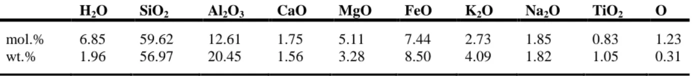
Table 1 - Starting bulk composition used in the construction of pseudosections and path-dependent P-T mode

diagrams in mol.% and wt.% from Yakymchuck & Brown (2014) as the average amphibolite-facies pelite from Ague ( 1991) after H2O adjustment to ensure minimal (<0.1 mol*.%) free H2O at the solidus at 12 kbar.

H2O SiO2 Al2O3 CaO MgO FeO K2O Na2O TiO2 O

mol.% 6.85 59.62 12.61 1.75 5.11 7.44 2.73 1.85 0.83 1.23

(27)

15 Fig. 4 - (a) Rcrust calculated NCKFMASHTO P-T pseudosection for the bulk composition in Table 1 with

arrows showing the P-T paths investigated by Yakymchuck & Brown (2014). (b) From Yakymchuck & Brown (2014) THERMOCALC one oxide normalised molar percentage of phases versus temperature for the path IBH12. (c) Rcrust calculated weight percentage of phases versus temperature for the path IBH12.

IBH = Isobaric heating, ITD = Isothermal decompression, ML = melt loss event. Abbreviations for rock forming minerals were taken from Whitney & Evans (2010) as: And = andalusite, Bt = biotite,Cpx = clinopyroxene, Crd = cordierite, Grt = garnet, H2O = water, Ilm = ilmenite, Kfs = alkali-feldspar, Ky = kyanite, Liq = liquid, Mag =

magnetite, Ms = muscovite, Opx = orthopyroxene, Pl = plagioclase feldspar, Qz = quartz, Sil = sillimanite, Spl = Spinel. Phase assemblages are as follows in addition to Pl and Ilm: 1-Bt,Ky,Ms,Mag,Qz ,

2-Bt,Grt,Ky,Ms,Mag,Qz , 3-2-Bt,Grt,Ky,Ms,Mag,Qz,H2O, 4-Bt,Grt,Ky,Ms,Qz,H2O, 5-Bt,Grt,Ky,Liq,Ms,Mag,Qz,

6-Bt,Kfs,Ky,Liq,Mag,Qz, 7-Bt,Ky,Liq,Mag,Qz, 8-Bt,Grt,Ky,Liq,Mag,Qz, 9-Bt,Grt,Kfs,Ky,Liq,Mag,Qz, 10-Bt,Grt,Kfs,Liq,Mag,Qz,Sil, 11-Bt,Kfs,Mag,Qz,Sil,H2O, 12-Bt,Ky,Ms,Qz,H2O, 13-Grt,Kfs,Liq,Sil,

14-Grt,Crd,Kfs,Liq,Sil, 15-Grt,Crd,Kfs,Liq, 16-Grt,Crd,Kfs,Liq,Qz,Sil, 17-Grt,Crd,Kfs,Liq,Mag,Qz, 18-Bt,Grt,Crd,Liq,Mag,Qz,Sil, 19-Bt,Crd,Liq,Mag,Qz,Sil, 20-Bt,Grt,Crd,Kfs,Liq,Mag,

21-Bt,Grt,Crd,Kfs,Liq,Mag,Opx, 22-Grt,Crd,Kfs,Liq,Mag,Opx, 23-Crd,Kfs,Liq,Mag,Opx, 24-Bt,Ms,Qz,Sil,H2O,

25-Bt,Crd,Kfs,Liq,Mag,Qz,Sil, 26-Bt,Kfs,Mag,Qz,Sil,H2O, 27-And,Bt,Kfs,Mag,Qz,H2O,

28-And,Bt,Crd,Kfs,Mag,Qz,H2O, 29-Bt,Crd,Kfs,Mag,Qz,Sil,H2O, 30-Bt,Crd,Liq,Mag, 31-Crd,Liq,Mag.

4.2. Reproducing the results of Yakymchuck & Brown (2014)

As a proof of concept study and to check the validity of Rcrust‘s calculations, the paths investigated by Yakymchuck & Brown (2014) were reinvestigated using Rcrust. The H2O

(28)

16 in the same NCKFMASHTO chemical system. The 2004 revised hp04ver.dat thermodynamic file was used with the internally consistent dataset of Holland & Powell (1998). Solution models were chosen which are consistent with the slightly simplified chemistry of the bulk system (e.g. the chemical system does not account for manganese) yet take into account substitutions that are important in stabilising phases (e.g. titanium in biotite). The following solution models were used: feldspar for plagioclase and alkali-feldspars (Fuhrman & Lindsley, 1988; Holland & Powell, 2003), Bio(TCC) for biotite (Tajcmanová et al., 2009), Mica(CHA) for other micas (Coggon & Holland, 2002; Auzanneau et al., 2010), hCrd for cordierite (Holland & Powell, 1998), Gt for garnet (WPH) (White et al., 2007), Opx(HP) for orthopyroxene (Powell & Holland, 1999), Cpx for clinopyroxene (HP) (Holland & Powell, 1996), Ilm(WPH) for ilmenite (White et al., 2000), melt(HP) for melt (Holland & Powell, 2001; White et al., 2001), Mt(W) for magnetite (Wood et al., 1991), Sp(HP) for spinel (Holland & Powell, 1998). Melt loss was set to occur when a 7 vol.% threshold of melt was exceeded and extraction left 1 vol.% behind approximating melt retained on grain boundaries. The Gibbs free energy minimisation method only considers discrete variation between arbitrary subdivisions within solid solution phases (pseudocompounds) with linear interpolation. Consequently, only a finite number of different phase proportions are produced resulting in slight variations in stable phase assemblages and their proportions between similar P-T conditions. Variation of stable phase assemblages introduce artefacts into pseudosections (Fig. 4a) while contrasting phase proportions at similar P-T conditions can offset threshold events blurring further boundaries (Fig. 7a). To alleviate these issues, we devised an approach called threshold buffering. Threshold buffering works by forcing the first time triggering of a threshold event to be postponed by a set number of points ensuring that the threshold is only triggered when it is consistently exceeded. The buffer is reset each time the threshold fails to be triggered (thus all boundaries are shifted by equal amounts). A resolution of 2 °C per point was used and a threshold buffering of 1 point (the system postpones extraction by 2 °C).

4.3. Comparing the results

Rcrust can output wt.%, mol.% or vol.% proportions. However, since volumes are pressure dependent plotting wt.% graphs yielded results most consistent with the case study (Fig. 4b & c). Phase proportions for the simple clockwise P-T paths show good agreement between the

(29)

17 simulations of Yakymchuck & Brown (2014) and that of Rcrust (Fig. 4b & c). Similar melt proportions are extracted at corresponding points on each P-T path. Minor differences are found for phase stabilities with Rcrust predicting clinopyroxene from 660 to 700 °C and a lower temperature sillimanite in boundary. These discrepancies are attributed to the difference in solution models chosen and updates in the thermodynamic dataset. However a key difference between the calculation methods is Rcrust‘s automated handling of a changing bulk composition

4.4. Clockwise P-T path

Each dependent path in Rcrust traverses a single line in P-T-X space and is not limited by the simple binary compositional range inherent to P-T, T-X or P-X diagrams. Individual paths allow investigation of phase proportions, compositions and the changing of a bulk

composition through path-dependent mode diagrams. To display the advanced functionality this provides, a clockwise P-T path is investigated with the same starting composition (Table 1), chemical system, solution models, 7 vol.% melt threshold, 1 vol.% melt retention and 1 point threshold buffering as used in Figure 4c. The clockwise P-T path (Fig. 5a) starts off with the same prograde heating segment as the high pressure (HP) path of Yakymchuck & Brown (2014) from 660 °C, 12 kbar to 860 °C, 18 kbar. This is followed by a retrograde P-T curve similar to those found by O'brien & Rötzler (2003) with near-isothermal decompression to 800 °C, 10 kbar and retrograde cooling until 550 °C, 6kbar. In Rcrust the entire clockwise

P-T path is calculated in one simulation with automated bulk compositional changes and

variations in P-T segments.

Phase proportions in the open system (Fig. 5e) show that melt loss decreases the ability of the reactive subsystem (RS) to form muscovite or increase the mode of biotite upon decompression. The solidus in the open system is crossed at 820 °C 12.8 kbar as opposed to 680 °C, 6.7 kbar in the closed system. This stabilises phase proportions along the retrograde path resulting in a fluid-absent subsolidus assemblage that preserves garnet, alkali-feldspar and a larger amount of sillimanite/kyanite (Fig. 5e). Only two melt loss events occur on the

P-T path, both at early stages of decompression, cumulating a total of 13 wt.% melt in the

extract subsystem (ES). To simulate the effects of local magma segregation, where magmas become chemically isolated from the reactive subsystem but remain in a relatively close position in the crus, the extract subsystem is calculated under the same P-T conditions of the reactive subsystem (RS) (Fig. 5f). Here the solidus is encountered at the onset of retrograde

(30)

18 cooling at 800 °C, 12 kbar forming a fluid-present subsolidus assemblage dominated by plagioclase feldspar, quartz, alkali-feldspar and orthopyroxene with minor amounts of muscovite, garnet and/or biotite at low temperatures (Fig. 5f).

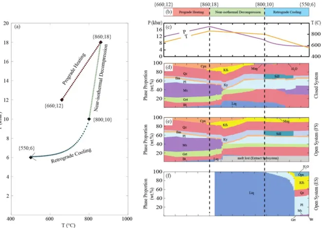
Fig. 5 - (a) Clockwise P-T path consisting of a prograde heating segment from 660 °C, 12 kbar to 860 °C, 18 kbar; followed by near-isothermal decompression to 800 °C, 10 kbar and retrograde cooling until 550 °C, 6kbar.

P-T values in Rcrust can be assigned by individual points or as functions of the number of steps in a P-T

segment. Thus the prograde heating and near-isothermal decompression segments were assigned values by linear functions of the form y = ax + y0 where y0 is the initial value and a is the gradient of the segment. The

retrograde cooling segment was assigned values by an exponential function of the form y = -b/c(1-e^(-cx)) + y0

where b and c are coefficients, y0 is the initial value and e is Euler's number. Black diamonds show P-T

conditions given in curly brackets as {T (°C);P (kbar)}. Circular dots along each path show individual

calculation points in Rcrust. (b) P-T segments with start and end P-T conditions for the clockwise P-T path. (c) Pressures (P) in purple and Temperatures (T) in orange, attained along segments of the clockwise P-T path. (d-f) Phase proportions along the clockwise P-T path for :(d) the closed system; (e) the open system (Full System) and (f) the open system (Extract Subsystem). Weight percentages are given relative to the Full System (FS) for (d & e) and only relative to the Extract Subsystem (ES) for (f). Abbreviations for rock forming minerals were taken from Whitney & Evans (2010) and are described in Figure 4.

(31)

19 4.5. Multi-path functionality

The compilation of multiple P-T-X paths can be used to create composite path-dependent P-T mode diagrams where a plane in P-T space is filled with points originating from dependent paths. These diagrams are limited to considering paths that are parallel in P-T space as the adjacency of points in the P-T plane must be maintained for readable outputs (when viewing the P-T plane orthogonally points cannot overlap).

This compilation method works by placing each point in a P-T-X path as sequential points in the column of a matrix. Each P-T-X path is placed in a new column. Starting conditions, bulk compositions and P-T-X event parameters can be scaled across the columns. Stable phase assemblages for each point are calculated and each unique assemblage is assigned an identification number.

The simplest form of these diagrams is when bulk composition remains constant across all P-T-X points, thus creating a normal P-T pseudosection. However, the Rcrust method is not restricted to keep bulk composition constant. Pressure, temperature and bulk composition can vary simultaneously within each P-T-X path allowing unique values to be attained dependent on the path taken. Path-dependence requires the diagrams be read in the direction of their constituent vectors, as events along the paths are not necessarily reversible on the path or scalable across paths. For example, when dealing with bulk compositional changes by melt loss events, we cannot assume that change through heating can be restored by cooling, nor can we assume that heating followed by decompression will result in the same bulk composition as decompression followed by heating. Points within a path are dependent on previous values therefore have to be determined in sequence. However if paths are set to be independent of one another they can be run in parallel threads to allow multiple calculations in the same simulation time.

4.6. Exploring new functionality

Multi-path functionality allows an array of isobaric heating paths to be examined. Melt loss events alter the bulk composition along the dependent paths, curving the P-T plane in the X dimension creating a path-dependent P-T mode diagram (Fig. 6d). The path-dependent P-T mode diagram in this case is dependent on bulk compositional changes encountered along the array of its constituent isobaric heating paths (grey arrows in Fig. 6d). For each point in the diagram, the amount of H2O depends on the cumulative bulk compositional changes

(32)

20 encountered by all points on the path before it. However each point on a path, is unaffected by points on adjacent paths. Thus the dependence of points relies on the direction of their constituent vectors. The reader must take note of the direction of the vectors and should be warned against false interpretations. These new path-dependent P-T mode diagrams provide a powerful tool which enables us to investigate the concepts proposed by Yakymchuck & Brown (2014) in more depth.

Fig. 6 - Contour plots of weight percentage (a) biotite, (b) muscovite and (c) total melt in the full system for the

closed system case. Values of zero are highlighted in grey for clarity. Contour values are given relative to the full system (FS) as indicated on the lower left hand side of each diagram. (d) Path-dependent P-T mode diagram from the compilation of isobaric heating paths starting with the composition in Table 1 at 640 °C followed by heating to 940 °C. Melt loss occurs whenever a 7 vol.% threshold is exceeded and leaves behind 1 vol.% melt approximating melt retention on grain boundaries. Grey arrows show the direction of constituent vectors (the isobaric heating paths). X scales the amount of H2O in the bulk composition of the reactive subsystem. Colour

(33)

21 5. RESULTS – EFFECTS OF MELT LOSS

5.1. Isobaric heating (IBH)

A path-dependent P-T mode diagram is created with melt extraction defined to occur whenever a 7 vol.% threshold is exceeded. When melt extraction is triggered all melt present in the reactive subsystem (RS) is extracted down to 1 vol.%. This approximates melt retention on grain boundaries. The melt extracts are stored in the extract subsystem (ES) that is independent from further P-T-X change and chemically isolated from the reactive subsystem. The same starting bulk composition, chemical system and solution models are used as described above. The path-dependent P-T mode diagram is built by combining parallel isobaric heating (IBH) paths from 2 to 12 kbar on the y-axis with a resolution of 141 paths each containing 141 points that span 640 to 920 °C on the x-axis (2 °C and 0.07 kbar per point with a threshold buffering of 1 point)(Fig. 7). These IBH mode diagrams can only be read from low temperature to high temperature as they are created by heating at fixed pressures. This is shown by the vector orientation at the top of Figs. 7, 9 & 10).

5.1.1. IBH interstitial melt

The amount of melt in the reactive subsystem (thus the interstitial melt) is contoured in Fig. 7a. The solidus is found on the left hand side of the diagram and is curved due to the pressure dependence of dissolved H2O in melt. For pressures above 6 kbar, the amount of interstitial

melt increases gradually up temperature to a local maximum at the boundary of the first threshold event (Fig 7a green contour with a positive slope intersecting at 780 °C, 12 kbar). At this boundary the interstitial amount exceeds the melt threshold of 7 vol.% so all melt except 1 vol.% is extracted. Heating beyond this boundary causes further melting and more extraction events producing a striped pattern of interstitial melt contours.

The low pressure range (<5 kbar) produces contrasting interstitial melt amounts at adjacent pressures. Areas which exceeded the threshold by a larger amount extract more interstitial melt initially which hinders further melting introducing lags in interstitial melt build up. This effect knocks on to points further along the path blurring the boundaries between extraction events at high temperatures and low pressures. As explained earlier this effect is somewhat lessened by the use of threshold buffering.

5.1.2. IBH total melt

The sum of the interstitial melt and the cumulative melt extracted along each path gives the total melt produced by the isobaric heating paths (Fig. 7b). Volume is pressure and temperature dependent necessitating the summing of melt extracts from a variety of P-T

(34)

22 conditions to be done on a mass basis. As a result the contour of total melt is plotted as the wt.% of melt relative to the full system (FS). The full system in this simulation consists of the reactive subsystem (RS) and the extract subsystem (ES). Contours scale total melt from close to 0 wt.% as red to 40 wt.% as green with null values highlighted in grey. The largest amount of total melt is found at the highest temperatures and lowest pressures. Contour shapes closely match that of the closed system total melt (Fig. 6c) but have a significant reduction in magnitude from a maximum of 60 wt.% to a maximum of 40 wt.%.

5.1.3. IBH residuum bulk H2O

For the P-T-X space investigated the bulk H2O content of the residuum is a major control on

its subsequent fertility. The amount of H2O in the bulk composition of the reactive subsystem

(RS) is contoured from close to 0 wt.% as red to 2 wt.% as green. Minimum residuum bulk H2O occurs at mid to high pressures (8 to 11 kbar) and the highest temperatures modelled

(Fig. 6c).

5.2. Isothermal decompression (ITD)

To complete the simple clockwise P-T investigation by Yakymchuck & Brown (2014) an isothermal decompression (ITD) path-dependent P-T mode diagram is created by projecting an array of parallel decompression paths down pressure from the 12 kbar isobaric heating path (IBH12). In these diagrams each point (for example the point at 780 °C, 7kbar in Fig. 7d) is reached by first following isobaric heating at 12 kbar until the point‘s temperature (here 780 °C) followed by isothermal decompression until the points pressure (here 7kbar). Thus points in the diagram can only be read going down pressure as shown by the vector orientation at the top of Figs. 7, 8, 9 & 10.

Melt extraction along the heating and decompression paths are defined by the same 7 vol.% threshold, 1 vol.% melt retained on grain boundaries and 1 point threshold

buffering as in the IBH system. Melt is extracted along the IBH12 path as well as along each

respective ITD path so an indication of the melt lost during the isobaric heating path is placed above the diagram (Fig. 7d). Melt lost is summed cumulatively on a weight basis and calculated relative to the full system (FS). Extraction events change the starting composition of decompressing paths, so for clarity in listing observations, the P-T space is classified into fields (with roman numerals) based on the amount of melt loss. The field bounds are: I (no melt loss) 640-780 °C; II (5 wt.%) 780-800 °C; III (10 wt.%) 800-840 °C; IV (15 wt.%) 840-870 °C, V (20 wt.%) 840-870-900 °C and VI (25 wt.%) >900 °C

(35)

23 Interstitial melt in Fig. 7d is contoured with the same scale as Fig. 7a to allow direct comparison. IBH12 melt loss fields are indicated with roman numerals. Boundaries to decompression melt extraction events occur at high angles to the constituent paths.

Paths that originate from the IBH12 path at temperatures below 800 °C have experienced 5 wt.% or less melt loss on the heating path (Fig. 7d I and II). These paths, upon decompression, show sequential melting zones bounded by melt thresholds.

Paths that originate above 800 °C have lost more than 5 wt.% melt on the IBH12 path. Melt loss events here break the interstitial melt contours into discrete fields which correspond with the IBH12 melt loss fields. Each of these fields starts off with melt present at 12kbar and has larger amounts of melt towards their respective high temperature boundaries. Decompression from 12 to 8 kbar, for fields between 800 and 900 °C (Fig. 7d III-V), decreases the amount of interstitial melt present. The decrease in interstitial melt upon decompression creates zones in P-T space where all melt in the reactive subsystem is crystallised. Melt is only encountered again after further decompression across a positively sloped line that intersects around 7.5 kbar and 920 °C. The >900 °C field (Fig. 7d VI) shows a slight increase in melt during decompression up to 7.5 kbar after which no interstitial melt is present until 2 kbar.

5.2.2. ITD total decompression melt

To highlight changes in decompression melt production the interstitial melt encountered along the ITD paths is summed with only the melt extracted during decompression (not including melt extracts from the IBH12 path)(Fig. 7e). Thus the total melt for each point in the P-T space can be found by adding the total decompression melt (Fig. 7e) to the IBH12 melt loss (above Fig. 7d). The maximum cumulative decompression melt formed in the given

P-T space (~25 wt.%. ) is found at 2 kbar at the high temperature end of the 780-800 °C field

(Fig. 7e II). The >900 °C field (Fig. 7eVI) does not experience melt loss events along any of its respective decompression paths.

5.2.3. ITD residuum bulk H2O

Decompression of the residuum at low total IBH12 melt loss (e.g. <800 °C Fig. 7f I & II) shows a systematic reduction in its bulk H2O content. Higher temperatures are associated

with more IBH12 melt loss and less decompression melt loss. Therefore decompression at higher temperatures has less of an effect on the residual bulk H2O content. The lowest bulk

H2O content is found in the >900 °C field (Fig. 7f VI) at ~0.07 wt.%. This value is constant

from 900 °C up temperature and down pressure as there are no decompression melt loss events in this field.

(36)

24 Fig. 7 - 7 vol.% threshold path-dependent P-T mode diagrams showing: (a,d) volume percentage melt in the

reactive subsystem (interstitial melt); (b,e) weight percentage melt in the full system (total melt); (c,f) weight percentage of H2O in the bulk composition of the reactive system (residuum) for the isobaric heating system

(IBH)(a-c) and the 12kbar isobaric heating followed by isothermal decompression system (ITD)(d-f). Values of zero are highlighted in grey for clarity. Contour values are given relative the reactive subsystem (RS) or the full system (FS) as indicated on the lower left hand side of each diagram.

(37)

25 5.3. Melt crystallisation zones

The close correlation between the bulk H2O content of the reactive subsystem and the amount

of interstitial melt in the reactive subsystem suggests, for this system at least, that H2O is a

limiting factor for melt production. In order to try explain the interesting decompression melt behaviour exhibited by the 7 vol.% threshold ITD system, the phase boundaries of the H2O

bearing phases muscovite, biotite and cordierite are plotted along with garnet and alkali- feldspar (Fig 8). The presence of interstitial melt is indicated by stippling and the garnet-biotite difference (the abundance of garnet minus the abundance of garnet-biotite both relative to the reactive subsystem) is contoured (Fig 8).

Heating along IBH12 initiates muscovite melting after 700 °C consuming muscovite, plagioclase and quartz (Fig. 8). At 12 kbar this melting produces only two melt extraction events (at 780 and 800 °C; Fig. 8 II & III) up to the muscovite-out-line at 800 °C. Cumulatively these events yield a maximum of 10 wt.% melt (Fig 8, Fig6 d). Further heating along IBH12 causes biotite melting (consuming biotite, plagioclase and quartz) across 3 melt extraction events (Fig. 8 IV-VI) forming a further 15 wt.% melt.

Decompression from the IBH12 path in the region before 780 °C encounters two decompression melt loss events due to muscovite melting before the muscovite-out-line followed by two decompression melt loss events after the cordierite-in-line where cordierite forms in favour of biotite (Fig. 8 I, Fig. 6d I).

Decompression in the 800-840 °C field (Fig. 8 III, Fig. 7d III) decreases the amount of interstitial melt in the reactive subsystem. This melt crystallisation corresponds to a shift in the garnet-biotite difference from 0 wt.% to -38 wt.%. This is thought to be the result of the thermodynamic system, upon decompression, using the H2O budget of the

system to form biotite at the expense of garnet and melt. After all the melt has crystallised the system continues to consume garnet (though in relatively smaller volumes for equivalent amounts of decompression) until the garnet-out-line around 7.5 kbar. Thus decompression melting in the 800-840 °C field (Fig. 8 III, Fig. 7d III) is only encountered again after 6 kbar of decompression when the cordierite-in-line is met.

Below the cordierite-in-line, cordierite and melt form in favour of biotite. Thus the high temperature side of the 800-840 °C field (Fig. 8 III) encounters a region where biotite, garnet, cordierite and melt coexist. The garnet-biotite difference in this region shows a shift from values near 0 wt.% to values close to -15 wt.% followed by an area of melt crystallisation. This shows again that if biotite, garnet and melt are present the system prefers biotite formation in favour of garnet thus melt crystallises upon decompression. This process

(38)

26 continues down pressure until all biotite is consumed at around 4 kbar (biotite-out-line)(Fig. 8 III).

Decompression in the 840-870 °C and 870-900 °C fields (Fig. 8 IV & V) encounter similar features however there is a greater abundance of biotite and lesser abundance of garnet thus shifts in the garnet-biotite difference are less drastic and a smaller amount of melt is crystallised.

In the field >900 °C (Fig. 8 VI) melt is the only H2O bearing phase above 7.5

kbar. Melt at lower pressures incorporates a lower amount of dissolved H2O consequently

decompression produces melting until the cordierite-in-line. Decompression across this boundary causes cordierite formation in favour of melt.

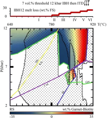
Fig. 8 - Phase boundaries and garnet-biotite mode difference for the 7 vol.% threshold 12kbar isobaric heating

followed by isothermal decompression system (ITD). Melt lost along the 12 kbar isobaric heating path (IBH12) is given above the main diagram as weight percentage relative to the Full System (FS). The temperature space is divided into zones based on the amount of melt extracted along IBH12 which are assigned roman numerals up temperature as: I (no melt loss) 640-780 °C; II (5 wt.%) 780-800 °C; III (10 wt.%) 800-840 °C; IV (15 wt.%) 840-870 °C, V (20 wt.%) 870-900 °C and VI (25 wt.%) >900 °C. On the main diagram garnet-biotite mode difference is contoured as weight percentage of the reactive subsystem (RS) from -35 wt.% difference (blue) where more biotite is present than garnet, through 0 wt.% difference (yellow) to 35 wt.% difference (red) where more garnet is present than biotite. The stippled area shows the presence of melt in reactive subsystem (RS). Boundaries of the garnet (green), muscovite/ alkali-feldspar (yellow), biotite (blue) and cordierite (purple) stability fields are shown as solid lines with labels placed on the side of the line where each phase is present.

(39)

27 5.4. Lower melt threshold investigation

If a lower melt threshold is considered, melt loss events will be more frequent but less voluminous, simulating a fractional melting scenario. If the melt threshold is equal to the melt retention amount, simulations will more closely approximate a ‗bleeding off‘ of melt once a connectivity transition is formed as opposed to pulses of melt that break the threshold (a batch melting scenario). To compare these behaviours path-dependent P-T mode diagrams are created with melt threshold and melt retention on grain boundaries both set to 1 vol.% (Fig. 9). For both the heating and decompression segments in these diagrams whenever 1 vol.% melt is exceeded all melt is extracted except 1 vol.%. The same P-T space, step size and threshold buffering is used as stated previously.

5.4.1. IBH interstitial melt (1 vol.% threshold)

Melt volumes exceed the threshold at the solidus attaining their maxima along its boundary (Fig. 9a). This triggers extraction which maintains a near constant 1 vol.% plane throughout the P-T space. Clusters of points at high temperature and mid to high pressures show melt crystallisation. Melt crystallisation is also found along the positive sloped cordierite-in-line (Fig. 8).

5.4.2. IBH total melt (1 vol.% threshold)

Total melt contours for 1 vol.% threshold (Fig. 9b) are near identical to that of the 7 vol.% threshold (Fig. 7b) with only a slight decrease in values at higher temperatures. A key difference however is that the melt extract contour (Supplementary Fig. 4b) is largely free of the distortions that are present in the 7 vol.% threshold melt extract contour (Supplementary Fig 2b). This is a result of the lower threshold having more frequent melt loss events so small offsets in P-T-X position of these events becomes less important. Threshold buffering is thus no longer necessary but is maintained at 1 point threshold buffering (2 °C and 0.07 kbar) for consistency between simulations.

5.4.3. IBH residuum bulk H2O (1 vol.% threshold)

Figure 9c shows that a lower threshold again has a smoothing effect where small pressure offset positions of extraction events are compensated by the multitude of events thereby preventing large knock on distortions seen at high temperatures in the 7 vol.% threshold plots (Fig 7c).

5.4.4. ITD interstitial melt (1 vol.% threshold)

IBH12 melt loss produces a more continuous accumulation of melt with constant gradients of melt loss maintained across the fields delineated by the 7 vol.% threshold system (above Figs.

(40)

28 7d and 9d). A relatively flat gradient of melt formation occurs between 700 and 800 °C (above Fig. 9d I and II) attaining a cumulative maximum of ~6 wt.% melt lost. This is followed by a sharp accumulation of melt at the muscovite-out-line up to 10 wt.% (Fig. 8, above Fig. 9d II). The 800-900 °C region shows a constant gradient across the fields III to V (above Fig. 9d) peaking at 23 wt.%. The gradient of the 800-900 °C region is stepper than the 700 to 800 °C region. The >900 °C field (Fig. 9d VI) shows an almost flat line with no further appreciable melt loss (maintaining a cumulative 23 wt.%).

Isothermal decompression (Fig. 9d) produces a similar 1 vol.% plane to IBH with a matching positive sloped line of melt crystallisation points on the cordierite-in-line (Fig. 8). At temperatures above 800 °C (>5 wt.% IBH12 melt loss) large melt crystallisation fields are found at 800-880 °C, 6-12 kbar and at 860-920 °C, 2-8 kbar. Melt volumes exceeding 1 vol.% occur on the low pressure boundaries of the first field. This occurs because the melt threshold is rapidly exceeded and threshold buffering only allows extraction one step after triggering of the threshold.

5.4.5. ITD total decompression melt (1 vol.% threshold)

Smaller more numerous melt loss events are encountered by the 1 vol.% threshold along IBH12 with a more incremental changing bulk composition. This more incremental change causes a more consistent reduction in decompression melt production with increasing temperature (Fig. 9e). Along the 2 kbar line, where the maximum amount of decompression melting has occurred along each respective path, the total decompression melt increases from 670 to 800 °C and then decreases from 800 to 920 °C. Maximum decompression melt is attained at 800 °C with ~23 wt.% (Fig. 9e). Melt crystallisation fields from the interstitial melt plot are still visible but are broken by vertical bands of constant amounts of melt by paths which exceeded the melt threshold before melt crystallisation began.

5.4.6. ITD residuum bulk H2O (1 vol.% threshold)

Residuum bulk H2O contents exhibit banding with vertically constant contents below 8 kbar

for temperatures above 890 °C and in the area 800-880 °C 6-12 kbar as no melt loss events occur in these regions. Apart from banding and a small region below the closed system solidus where decompression paths maintain their melting history (by having lower bulk H2O