ATM network striping

(1)

ATM Network Striping

by

Michael Ismert

Submitted to the Department of Electrical Engineering and Computer Science in partial fulfillment of the requirements for the degree of

Master of Engineering in Electrical Science and Engineering at the

MASSACHUSETTS INSTITUTE OF TECHNOLOGY

February 1995

The author hereby grants to MIT permission to reproduce and to distribute copies of this thesis document in whole or in part, and to grant others the right to do so.

A u th o r ...

Department of Electrical Engineering and Computer Science February 6, 1995

Certified by... .... ... ... . . .n.u....v. L.

David L. Tennenhouse

Associate Professor

Accepted by...

of Computer Science and Engineering Thesis Supervisor

..

.

. . ..

. .... . . . .. .. . . . .. . . ...

Frederic

R. Morgenthaler Chairman, Departmental Cnmittee on Graduate Students

MASSACHUSETTS INSTITUTE OF TECHNOLOGY

AUG 10 1995

LIBRARIES

(2)

ATM Network Striping

by

Michael Ismert

Submitted to the Department of Electrical Engineering and Computer Science on February 6, 1995, in partial fulfillment of the

requirements for the degree of

Master of Engineering in Electrical Science and Engineering

Abstract

There is currently a scaling mismatch between local area networks and the wide area fa-cilities provided by the telephone carriers. Local area networks cost much less to upgrade and maintain than the wide area facilities. Telephone companies will only upgrade their facilities when the aggregate demand of their customers is large enough to recover their investment. Users of LANs who want a wide area connection find themselves in a position where they are unable to get the amount of bandwidth they need or want at a cost that is acceptable. This coupling of technology in the two domains is a barrier to innovation and migration to new equipment.

Network striping is a method which will decouple the progress of technology in the local

area from progress in the wide area. This thesis proposes a reference model for striping in a network based on Asynchronous Transfer Mode (ATM). The model is used to analyze the degrees of freedom in implementing network striping, as well as the related issues and tradeoffs. An environment that interconnects three different ATM platforms has been used to explore and experiment with the functional space mapped out by the model. The results are used to validate and improve the predictions of the model.

Thesis Supervisor: David L. Tennenhouse

(3)

4.2 Interesting Cases . . . . 4.3 Conclusion . . . . . . . 5 Experimental Apparatus 15 . . . . 1 6 . . . . 1 8 . . . . 1 9 . . . . 2 0 . . . . 26 27 . . . . 27 . . . . 32 . . . . 36 . . . . 38 . . . . 40 . . . . 41 . . . . . . . . . . . .

(4)

5.1 VuNet ... ... 48

5.2 A N2 . . . .. .. . . . .. ... .. . . . .. . 51

5.3 Aurora .. . . . . .. . ... .. . .. .. . .. . . . .. .. . ... ... .. 52

5.4 The W hole Picture . . . . 54

6 The Zebra 56 6.1 Initial Design Issues . . . . 56

6.2 Zebra Design Description . . . . 58

6.3 Sum m ary . . . . 69

7 ATM Layer Striping 70 7.1 Synchronization Options . . . . 70

7.2 Header Tagging . . . . 72

7.3 Payload Tagging . . . . 74

7.4 VPI Header Tagging . . . . 76

7.5 Header Metaframing . . . . 77

7.6 Payload Metaframing . . . . 80

7.7 Hybrid M etaframing . . . . 80

7.8 Dynamically Reconfiguring the Number of Stripes . . . . 83

7.9 Load Balancing . . . . 83

7.10 Experimental Implementation and Results . . . . 85

7.11 Conclusion . . . . 89

8 Striping at Upper Layers 91 8.1 Adaptation Layer Striping . . . . 91

8.2 Network Layer Striping . . . . 93

8.3 Transport Layer Striping. . . . . 95

8.4 Application Layer Striping . . . . 96

8.5 Conclusion . . . . 96

9 Conclusion 98 9.1 Striping Framework .... ... ... ... ... .. .. 98

9.2 The Case for ATM Layer Striping .... ... .... . . . .. ... . .. 100

(5)

A Justification for Unconsidered Striping Cases 102

B Xilinx Schematics 105

B.1 AN2-Bound/VuNet Side Xilinx - Input Pins . . . . 106

B.2 AN2-Bound/VuNet Side Xilinx - Output Pins . . . . . . . . . . . . . . 107

B.3 AN2-Bound/VuNet Side Xilinx - Data Path . . . . 108

B.4 AN2-Bound/VuNet Side Xilinx - FSM . . . . 109

B.5 AN2-Bound/AN2 Side Xilinx -Input Pins . . . . 110

B.6 AN2-Bound/AN2 Side Xilinx - Output Pins . . . 111

B.7 AN2-Bound/AN2 Side Xilinx - Data Path . . . . 112

B.8 AN2-Bound/AN2 Side Xilinx - FSM . . . . 113

B.9 VuNet-Bound/AN2 Side Xilinx - Input Pins . . . . 114

B.10 VuNet-Bound/AN2 Side Xilinx - Output Data Pins . . . . 115

B.11 VuNet-Bound/AN2 Side Xilinx - Output Control Pins . . . . 116

B.12 VuNet-Bound/AN2 Side Xilinx - Data Path . . . . 117

B.13 VuNet-Bound/AN2 Side Xilinx - FSM . . . . 118

B.14 VuNet-Bound/VuNet Side Xilinx - Input Pins . . . . 119

B.15 VuNet-Bound/VuNet Side Xilinx - Output Pins . . . . 120

B.16 VuNet-Bound/VuNet Side Xilinx - Data Path . . . . 121

B.17 VuNet-Bound/VuNet Side Xilinx - FSM . . . . 122

C Zebra Schematics 123 C.1 ECL - G-Link Interface . . . . 124

C.2 ECL -AN2-Bound Direction . . . . 125

C.3 ECL -VuNet-Bound Registers . . . . 126

C.4 ECL -VuNet-Bound Multiplexors . . . . 127

C.5 ECL -Miscellaneous Components . . . . 128

C.6 TTL -AN2-Bound/VuNet Side . . . . 129

C.7 TTL -VuNet-Bound/VuNet Side . . . . 130

C.8 TTL -AN2-Bound and VuNet-Bound/AN2 Side . . . . 131

C.9 TTL -AN2 Daughtercard Interface . . . . 132

(6)

List of Figures

1-1 Network Striping Experimental Apparatus . . . .

2-1 2-2 2-3 2-4 2-5 2-6 3-1 3-2 3-3 3-4 End-to-end Topology . . . .

Fully Internal Topology . . . . . . .

Hybrid Topology . . . .

Identifying Striping Units by Protocol Layer . . . . . Improper Reassembly Due to a Lost Striping Unit

Improper Reassembly Due to Skew . . . .

Tagging Striping Units Across the Stripes . . . .

Tagging Striping Units on Individual Stripes . . . .

Using Striping Elements with Metaframing Patterns

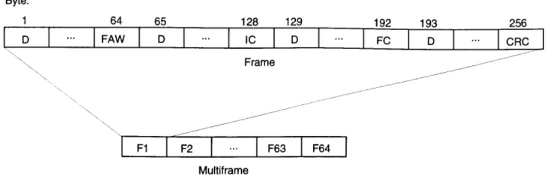
BONDING Frame/Multiframe Structure . . . .

5-1 Sample VuNet Topology . . . .

5-2 Example of an AN2 Node . . . .

5-3 Aurora Testbed Participants . . . .

5-4 VuNet/AN2/Sunshine Topology . . . .

6-1 Final Path between the VuNet and AN2 through the Zebra 6-2 Top-Level Zebra Block Diagram . . . . 6-3 AN2-Bound/VuNet Side Block Diagram . . . .

6-4 AN2-Bound/AN2 Side Block Diagram . . . .

6-5 VuNet-Bound/AN2 Side Block Diagram . . . . 6-6 VuNet-Bound/VuNet Side Block Diagram . . . .

7-1 Payload Tagging . . . . . . . . . . . . . 17 . . . . 17 . . . . 17 . . . . 20 . . . . 25 . . . . 26 . . . . . . . . . 49 . . . . 51 . . . . 53 . . . . 55 . . . . 57 . . . . 59 . . . . 60 . . . . 62 . . . . 65 . . . . 66 . . . . 75

(7)

7-2 VPI Header Tagging . . . . 77

7-3 Header Metaframing using Pairs of VCs . . . . 78

7-4 Hybrid Metaframing . . . . 81

(8)

List of Tables

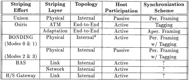
3.1 Striping Cases Explored by Previous Efforts . . . . 42

4.1 Initial Striping Space . . . . 44

4.2 Interesting Cases . . . . 46

(9)

Chapter 1 Introduction

This thesis examines the use of network striping as a means to increase network performance

without requiring the entire network to be upgraded. Network striping, also referred to as

inverse multiplexing, is the use of multiple low speed channels through a network in parallel to provide a high speed channel. Our examination of striping is done in two parts. First, a reference model will present the degrees of freedom characterizing a network striping

implementation. The model will be used to identify several interesting and previously unexplored striping cases. These cases will be examined in greater detail to see how they

could be implemented and to determine what other requirements are needed from the hosts

and the networks in order to make these striping cases function properly.

Along with the theoretical work, a set of experimental apparatus has been developed

to actually explore some of the striping cases which have been identified. The apparatus

consists of an experimental ATM-based gigabit desk-area network connected to a high-speed ATM-based local-area network which is then connected to wide-area SONET facilities.

1.1 Motivations for Network Striping

The main factor limiting progress in the wide area is scale. Due to the large scale, it costs a

great deal of money, time, and effort to install and upgrade equipment. Thus, the telephone companies can only afford to upgrade their equipment relatively infrequently. In order to recover their costs, the telcos only upgrade when they believe that there is sufficient demand for new or improved service. They also upgrade to a much higher level of service, which allows them to meet increasing demands for bandwidth for a long period of time. For

(10)

example, the digital hierarchy originally used by the telcos provides channels at 64 kbps

(DSO), 1.544 Mbps (DS1), and 45 Mbps (DS3)[1]. As equipment is upgraded to SONET,

155 Mbps (OC-3) will be the next level of service provided, with 622 Mbps (OC-12) as the next probable upgrade. It takes a great deal of time for the entire network to be upgraded. Initially only the links in the center of the network which carry the heaviest traffic will be replaced; upgraded links will slowly diffuse out to the edges of the telephone network as demand grows and time and money permit them to be replaced.

The main factor limiting progress in the local area is technological progress. Because of the smaller scope, the cost of installing and maintaining a LAN is relatively low. As

soon as a new network technology becomes well-developed and supported, early adopters

will begin to upgrade their LANs. It is even feasible for research groups to design and

deploy their own custom LANs. The wide range of LAN technologies means a wide range

of LAN speeds, ranging from 10 Mbps Ethernet to 100 Mbps FDDI and Fast Ethernet to gigabit-per-second custom LANs.

The differences between wide and local area networking create several major problems when the two domains are interconnected. First, the bandwidth numbers don't match up

very well, leading to inefficient use of either network or monetary resources. Bandwidth in

the wide area is governed by a strict hierarchy, where each level is some fixed multiple of the previous level with the addition of some extra signalling and synchronization information.

Local area bandwidth is much more flexible, where functionality or available technology is

the driving factor. LAN users will frequently find themselves stuck between two levels of the hierarchy, with two options available to them. They may opt for the lower level and

settle for less available bandwidth over the wide area. They may opt for the higher level, but they will then pay a higher price for more bandwidth than they require. High-end users with custom LANs will find themselves out of the hierarchy completely, above the highest level of service that the telcos currently provide, and will have to settle for insufficient bandwidth. In the past, LAN users could accept the lower wide area bandwidth, making the valid assumption that only a fraction of the traffic on the LAN would be bound for the wide area. However, inter-domain traffic is increasing as the World Wide Web grows and becomes more popular as a means of gathering information. Video distribution applications such as the MBone[2] and the WWW Media Gateway[3] not only contribute to the inter-domain traffic, but create a demand for high bandwidth connections which serve very few

(11)

users at a time.

In many cases, the links within the telephone network may have enough raw capacity to handle a high bandwidth connection; unfortunately, the links are partitioned into smaller logical channels which cannot provide the necessary bandwidth. The size of these channels is determined by the amount of bandwidth which the average user needs or wants. Higher bandwidth channels are simply not available. Even though the entire path between two geographically separate hosts may have the aggregate capacity to support their high band-width applications, each point along the path must also be upgraded to support a higher level of service for the average user.

There is yet another problem created by the local access to the telephone network. The connection between the LAN and the telephone network must be able to support the amount of bandwidth which the users need. This may not be something which the local provider is able or willing to do. For example, someone wanting OC-12 access to the telephone network may get it in one of three forms. They may be provided with a single connection which gives them access to a single 622 Mbps channel. This is the optimal situation from the user's standpoint but also the most difficult for the local provider to offer and support. The user may be provided with a single connection which gives them access to 622 Mbps in the form of four 155 Mbps OC-3 channels. These four channels may be co-located on one fiber or may be four separate fibers. This would be the case if the local provider's equipment was only able to handle channels at the OC-3 level or below. Finally, the user could be provided with a 622 Mbps channel onto their premises with an OC-12/OC-3 demultiplexor

that provided them with access to four separate OC-3 channels. This would be the case if the local provider was only able to handle OC-3 channels and only allowed OC-12 links that were internal to their network. Either of the last two cases would allow a single application access to only 155 Mbps.

The differences also create a coupling effect which slows the migration to new technol-ogy in both domains. When a company or research group upgrades their LAN, they will immediately see increased performance locally. However, performance across the wide area will probably change very little, if at all. This is unfortunate, particularly if the company has several geographically separated sites which have upgraded their LANs; the individual sites have better network performance, but their interoperation is limited by the wide area facilities. The company will either need to lease higher speed lines from the telcos, which

(12)

will probably provide significantly more bandwidth than necessary, or wait for the telcos to upgrade their equipment so that the required bandwidth to connect the sites is

avail-able. These factors act as a deterrent for groups to upgrade their LANs until the wide area

services they want are available and slows progress in the local area. The telcos will delay providing improved service until there is a sufficient demand for it. This slows progress in

the wide area.

1.2 Network Striping

Any new wide/local area interoperation scheme should have two properties. First, it should

have the flexibility to provide LAN users with whatever reasonable amount of bandwidth

that they require. For example, 10 Mbps Ethernet users should have access to 10 Mbps of wide area bandwidth, not 1.544 Mbps or 45 Mbps. High-end users should have some way to

get the bandwidth which they require as well. This will allow LAN and wide area facilities

to be used more efficiently and will reduce costs for the telco customers.

The scheme should also have the ability to decouple LAN and wide area progress. This

includes solving the problem of a path which has not been completely upgraded. Users of

upgraded LANs should be able to see immediate benefits when interoperating with other upgraded LANs, even across the wide area facilities. This is currently the situation with

modem technology; anyone purchasing an new modem can plug it in and instantly get higher performance with anyone else who has a fast modem. In addition, it would also be

desirable for the scheme to be as independent of the physical network equipment as possible;

this will allow migration to improved technology to be made very easily.

A scheme which can support these properties is network striping. Network striping

uses multiple low speed channels through a network in parallel to provide a high speed

channel. It provides the desired bandwidth flexibility by allowing the use of as many low speed channels, called stripes, as necessary, assuming that the channels are available. The

ability to add and remove stripes as desired also provides the decoupling between the local and wide areas by allowing users with upgraded LANs to simply increase the number of stripes they are using tp increase the bandwidth available to them.

Of course, there are advantages and disadvantages to network striping. In addition to

(13)

bandwidth available not only when they upgrade their LANs, but also to change the number of stripes used dynamically as the amount of traffic increases or decreases. This would be

particularly useful in the case where there are usage charges on each stripe. Network striping

also provides for some protection against network failures. If the bandwidth through the wide area is provided by one channel, if this channel fails, then there is no connectivity until it is repaired or replaced. If one of the channels in a striped connection fails, the connection

will still be intact, just at reduced bandwidth. On the negative side, while network striping will provide high bandwidth to those users and applications which require it, it incurs a

cost in complexity; it requires more work to send data over several channels in parallel than

to just send data over one channel.

1.2.1 ATM and Network Striping

A large portion of this thesis addresses network striping as it may exist in an Asynchronous

Transfer Mode[4] environment. One might argue that ATM will, in theory, be able to provide solutions to the same problems which network striping is attempting to solve. Users should

be able to request virtual circuits with the amount of bandwidth they require, providing

both the flexibility and the decoupling desired. However, there are still cases motivating

the use of network striping with ATM. Virtual circuits provided by ATM will be limited

to the amount of bandwidth which the physical channels can carry. Any user who wishes more bandwidth than that will need to use multiple physical channels, which is striping.

1.3 Contents of this Thesis

This introduction has provided justification for examining network striping in more detail. Chapter 2 will describe a framework with which all striping designs can be categorized and

analyzed. In addition to the framework, Chapter 3 contains some previous work related to network striping and some of the tools available to solve the problems associated with it. Chapter 4 uses the framework to present all the possible striping cases; from these we have selected a few which we analyze in greater detail.

Chapters 5 and 6 will present the details of the existing experimental environment and the custom hardware which was developed to allow a complete interconnection. This

(14)

To Sunshine switches

VuNet Lik Zba AN2 4sO 003 Sunshine and other VuNet nodes

Switch Switch Line Ca Switch at Bellcore, UPenn.

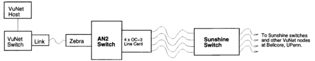
Figure 1-1: Network Striping Experimental Apparatus

experimental desk-area network developed at MIT. It is connected to AN2, a local-area

network developed by Digital, through a piece of custom hardware called the Zebra. AN2 is connected to the Aurora[5] testbed's wide-area facilities through a 4 x OC-3c line card on

the AN2 which is connected to an experimental OC-3c to OC-12 multiplexor developed by

Bellcore. The OC-12 multiplexor can connect either directly to the facilities or to another

OC-12 multiplexor attached to Bellcore's Sunshine switch[6].

Following the description of the experimental apparatus, the analysis of the remaining

striping cases, along with some experimental results, is presented in Chapters 7 and 8. We will show that the ATM layer is an appropriate layer at which to implement striping. Lower

layer striping is very constrained by the network equipment, while higher layer striping

provides benefits only to those using that protocol. Finally, we state our conclusions and

(15)

Chapter 2 Striping Framework

Our goal is to identify and examine a subset of the possible striping cases which meet the

criteria in the previous chapter. The first task, then, is to characterize the important aspects

of any striping implementation so that all the cases can be easily identified. This chapter will present a general framework which we will use as a means to consistently describe possible

striping implementations. As part of this framework, we will identify several degrees of freedom which capture all the important aspects of a particular striping implementation.

To be certain that all the striping cases are covered by the framework, consider how

an arbitrary striping implementation might function. The connection between the source

and destination hosts must be split into stripes somewhere along the route. The possible places in the network where this split may occur will affect how the striping implementation

functions. We will refer to this as the striping topology and it will be the first degree of

freedom.

Since it is the hosts at the edges of the network that are going to benefit from striping, the next thing to consider is the role that the hosts play in the striping implementation.

This will be affected by the striping topology; in some cases the topology may dictate that

the hosts may be required to be completely responsible for implementing the striping while in others they can be completely unaware of it.

Once the striping topology is known and the hosts' places in it are determined, data

could potentially be striped. In order for this to happen, the data which is being transmitted

by the hosts needs to be broken up into pieces which are then transmitted along the stripes

(16)

unit is actually a subset of issues associated with the network layer at which the striping

is implemented. The striping layer is affected by both of the previous degrees of freedom. For example, if the hosts are performing the striping, then the network to which they are

connected affects the possible striping layer. If the striping is completely internal to the network then only the portion of the network over which the striping occurs affects the striping layer.

The three elements above allow the description of the most basic striping implementa-tions, under ideal conditions. However, network conditions are rarely ideal, and so we will consider what difficulties must be dealt with in order to insure that a striping implemen-tation will function correctly. Many difficulties associated with striping are the result of

skew. Skew is a variation in the time it takes a striping unit to travel between the

trans-mitting and receiving hosts on different stripes. The combination of skew and data loss will

cause data to be delivered out of order and make it necessary to implement some sort of

synchronization across the stripes to determine the correct order at the receiver.

The remainder of the chapter will examine each of the degrees of freedom in more detail, determining the various possibilities for each and examining how they affect each other.

2.1 Striping Topology

The first degree of freedom we will consider is that of striping topology. This is the

descrip-tion of where the path between two hosts is split into stripes. There are two basic reference topologies. In the simplest case, the connection is completely split into stripes from one

end to the other; this is the end-to-end splitting case. In the second case, the connection is

split between two nodes in the network; this is the internal splitting case.

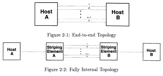
2.1.1 End-to-End Splitting

The end-to-end splitting topology is shown in Figure 2-1. This topology is the simplest to analyze because the stripes are discrete physical channels for the entire length of the connection; there is no opportunity for units on different stripes to mingle or suffer from routing confusion. However, it is very rare that two end-systems are fully connected by several stripes; almost all LAN-based hosts are connected to a network through just one physical interface.

(17)

2

Host

A

B

Figure 2-1: End-to-end Topology

Striping 2 Striping

Host Element Element Host

A B B

Figure 2-2: Fully Internal Topology

2.1.2 Internal Splitting

Figure 2-2 shows the internal splitting topology. This case is far more likely to exist; each host has only one connection to the network which then provides multiple possible paths between the source and destination. Unlike the end-to-end case, this topology adds the complexity of considering the effects of routing decisions at the point where the network is split to the analysis.

As network links are slowly upgraded, we expect that sections of paths between hosts will be collapsed into single channels. This will lead to striping topologies with cascades of internal splitting.

2.1.3 Combinations

The end-to-end and internal cases are the two simplest possible topologies; there are, of course, a large variety of topologies which may actually exist. For example, the hybrid topology (Figure 2-3) is half of the internal and half of the end-to-end topologies. This case could be applied to the rare case of an end-system with a normal network connection communicating with a host with multiple network connections.

Even more complex topologies are possible; as networks grow and paths added to provide redundant routes, a potential web of connections between any two geographically separate

1

Host Striping -2 Host

A

Element

-

B

(18)

hosts will exist. However, we will concern ourselves mainly with the two basic cases above, addressing more complex topology issues only when necessary.

2.2 Participation

An important aspect of a striping implementation is the role which the end-systems and

networks play. The striping may occur without the knowledge of the end-systems; we will

refer to this as the passive case. The other possibility is that the end-systems must perform

some of the functions of the striping implementation. This will be referred to as the active

case.

2.2.1 Passive End-Systems

In the passive case, the hosts are not aware that any striping occurs. This has the advantage

that the hosts need not do anything special to transmit to any host, whether or not the two are connected through stripes. This allows the use of current host software, as well as

reducing the overhead required in order to implement the striping. However, passive striping

requires that the network handle the entire striping implementation, requiring more complex network equipment and/or modifications to the existing equipment.

Obviously, this case is limited to the internal and hybrid splitting network topologies. Thus, any time we refer to the passive case, we will assume that the striping topology is

internal.

2.2.2 Active End-Systems

In the active case, the hosts are responsible for some part of the striping. This responsibility

for the transmitting host can vary from handling the entire striping implementation to merely providing information to allow the network to properly carry out striping, depending on the other degrees of freedom. In almost all cases, it will be the responsibility of the

receiving host to properly reassemble the striped data from the transmitter. The tradeoffs here are essentially the opposite of those in the passive case; the hosts require new software but the portion of the network containing stripes can use existing equipment.

Any time the topology is an end-to-end split, the hosts must handle all of the striping implementation.

(19)

2.2.3 Network Participation

The networks also play a role in any striping implementation. They implement the parts of the striping implementation not performed by the hosts. In the passive case, the network must handle the entire implementation, while in the active case, the responsibility may be shared in some way. In addition, since the network is providing the paths over which the striping is performed, an important part of a striping implementation is the guarantees which the hosts have from the network.

2.3 Striping Layer

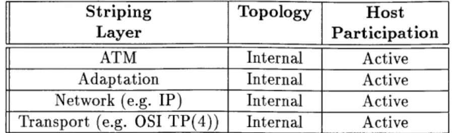
As striping is a network function, there must be some way to associate it with the layers of the OSI network protocol stack. The networks over which the striping occurs will de-termine the possible layers at which striping can be performed. The lowest layer which is

homogeneous across the portion of the network involved in the striping implementation is

the lowest possible striping layer. In the passive striping case, only the network between the two points which handle the striping needs to be homogeneous at the striping layer; in the active case, the entire network between the source and destination must be homogeneous at

the striping layer. An interesting thing to notice is that only the striping layer is required

to be homogeneous; the layers above and below can be virtually anything. For example, striping at the ATM layer will support any combination of network layers and will operate using any combination of physical layers; striping at the network layer will support any combination of technologies which provides that layer.

2.3.1 Striping Unit

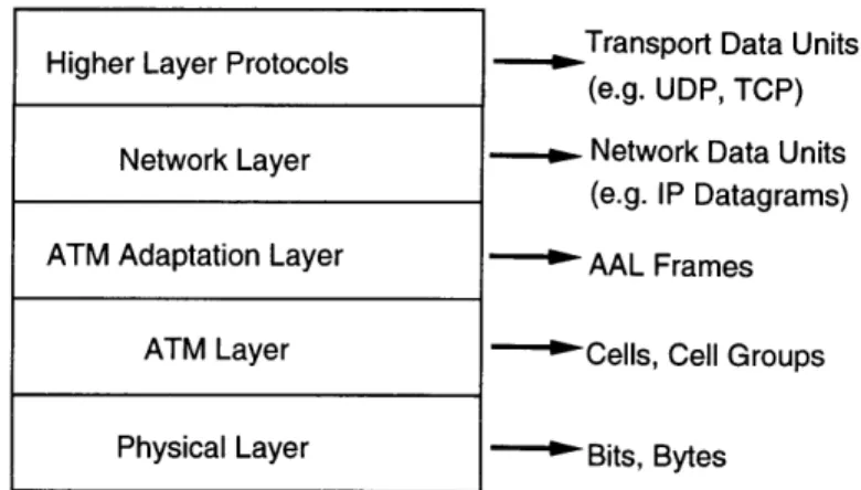
After determining the possible striping layers, we can make a list of the available striping elements. Figure 2-4 shows the striping units associated with the most likely layers in the ATM protocol stack.

Note that while the figure only shows striping units for the transport layer and below, the same idea holds all the way up to the application layer.

(20)

Transport Data Units

Higher Layer Protocols

(e.g. UDP, TCP)

Network Data Units

(e.g. IP Datagrams)

ATM Adaptation Layer AAL Frames

ATM Layer - Cells, Cell Groups

Physical Layer _{Bits, Bytes}

Figure 2-4: Identifying Striping Units by Protocol Layer

2.4 Implementation Issues

The previous degrees of freedom can be viewed as situational and architectural; they are concerned with aspects of striping which are probably not completely under the control of someone designing a striping implementation. Next, we will look at some implementation issues; things with which, given the situation, the designer has to be concerned.

2.4.1 Striping Unit Effects

One characteristic of the striping units at different levels is that they differ in bit length.

This will have some profound effects on the network and on performance, which will be explored below.

Throughput and Packetization Delay

As the bit length of the striping unit varies, it will affect the throughput of amounts of data which do not require the use of all the available stripes. The aggregate throughput seen

by bursts of data many striping units in length will be the sum of the throughputs of all

the stripes. However, single striping units which are not transmitted in bursts will only see the throughput provided by the stripe on which they are transmitted. As the size of the striping unit increases, the hosts must be able to generate larger bursts of data in order to see the benefits provided by striping.

Similarly, as the size of the striping unit varies, the latency due to packetization delay increases. This effect occurs even with the use of a single channel, but it is aggravated

by the fact that although the stripes provide an aggregate bandwidth equal to the sum of

(21)

the bandwidths, the packetization delay is determined by the bandwidth of an individual

stripe. For example, the packetization delay of a 1000 bit striping unit on a single channel providing 100 Mbps is 10 psec. However, if four 25 Mbps stripes are providing the same amount of aggregate bandwidth, the packetization delay will be the packetization delay of the individual stripes, which is 40 psec.

Unbalanced Loads

The two previous effects were due to an overall change in length due to varying the striping unit. Some striping units may have the characteristic that their length may vary; for example, naively striping variable length IP packets at the network layer will result in each stripe carrying packets of differing lengths. Under some conditions, this could cause some stripes to be overwhelmed with traffic while others go grossly underutilized; as a simple example, take the case where small and large packets arrive in an alternating pattern to be striped over an even number of stripes. This problem is due to the simple round robin strategy used to deliver the packets to the stripes; we can potentially modify the round robin process to balance the load on each stripe1_.

One such modification, Deficit Round Robin[7], can be shown to provide the load bal-ancing required. In this case, each stripe has a balance of bytes which it may take, some of which may be left over from previous rounds. At the start of a new round, a fixed quantity of bytes is added to the balance for each stripe. The standard round robin algorithm then proceeds with the following modifications. The size of an element placed on the current stripe is subtracted from its balance. If the new balance is larger than the size of the next element, then the next element is also transmitted on that stripe. This process repeats until the balance for the stripe is lower than the size of the next element. At this point, the same procedure begins with the next stripe.

Effect of the Striping Unit on Synchronization

The striping units at each layer have widely different formats. Aside from the bit/byte

layer, all of them have some sort of header or trailer with various fields used to manage that layer. In addition, each layer is handled in a different fashion both by the nodes in

Modifying the round robin process to perform load balancing will at least restrict the synchronization options available at the receiver, and possibly make a more sophisticated scheme necessary.

(22)

the network as well as by the hosts. The layer overhead is one place where synchronization information may be placed, and the layer specifies how the receiver will handle the incoming striping unit. This will cause the details of striping implementations at each layer to vary quite a bit as well, which will be seen in greater detail below.

2.4.2 Skew and the Need for Synchronization

As stated earlier, skew is a difference between the travel time on two stripes. Suppose that sources submit striping units to the stripes in a round robin order. The receiver will expect them to arrive in the same order2_{. Differences in the paths traversed by each stripe can} introduce skew between the stripes and cause the striping units to arrive at the destination

misordered.

There are three main causes of skew. These are the physical paths of each of the stripes, the multiplexing equipment which carry the physical channels, and switching ele-ments through which each stripe passes. Different physical paths introduce skew by having different propagation delays due to traveling different distances. For example, if a striped connection between Boston and Seattle has two stripes which are routed directly between the two cities and two stripes which must pass through Dallas, then the transmission delay of the second pair of stripes will be longer simply because the path that they have to travel is longer.

Even if the stripes are constrained to follow the same physical path between the source and destination, skew may still be introduced by the multiplexing equipment along the route of the stripes. This is the case in the Aurora testbed, where the manipulation of the separate OC-3c channels in the OC-12 connections by the transmission and multiplexing equipment was enough to introduce skew between the SONET payloads3_{. Finally, switching}

elements may cause an even greater amount of skew if they introduce different queueing delays on each stripe.

Skew Assessment

When we begin to discuss some striping cases in more detail, we will want some idea of the worst case skew which will be introduced by the network. We can measure skew in two

2

We will refer to one cycle by the transmitter or receiver through all the stripes as a round.

3

(23)

different forms; for an absolute sort of measure we can consider skew as an amount of time in seconds. However, when considering how to design a synchronization method to protect against skew, we will want to know the amount of skew in terms of striping unit times; that is, how many striping elements can be received by the destination in the amount of skew time. We will consider the absolute skew introduced by the path difference, multiplexing equipment, and queueing delay separately, and then convert these times into striping unit times.

The amount of skew introduced by different physical path lengths depends upon the transmission media. We will assume the media to be optical fiber, which has a propagation delay of 7.5 ps per mile. If the difference in path length is M miles, then the skew introduced

by this length is 7.5 x Mps. For example, if we consider the worst case path length difference

in the U.S. to be about 1000 miles, then the skew this introduces will be 7.5 ms. On a world-wide scale, we might expect the worst case path difference to be as large as three or four thousand miles, or 30 ms. This amount of skew is fixed as long as the paths remain the same.

The amount of skew introduced due to the multiplexing equipment depends on the number of multiplexors in the path. We expect this skew to be relatively small based on our experimental results at the ATM layer, which we will present in chapter 7. Two co-routed OC-3c channels passing through 8 OC-3c/OC-48 multiplexors, a distance of approximately

500 miles, suffer a skew of only one cell time, which is approximately 2.2ps. Since we do not expect significantly more multiplexors to be present on a channel of longer length, we will assume the worst case skew introduced by the multiplexing equipment to be less than an order of magnitude greater, around 11ps. We expect that this skew will not vary much, remaining constant for long periods of time.

If the striping is performed at or about the network switching layer, then there will also

be skew due to variable queue lengths on each path. The skew due to queueing delay will tend to vary quite a bit. If we assume two striping units arrive at two different switch ports which are each capable of buffering b striping units, then the worst difference in queue length which these two units will see is b. We can calculate the approximate skew introduced by this queue difference by calculating the time it takes for one striping unit to be removed from the queue. This will be approximately the size of the striping unit divided by the

(24)

Skew vs. Data Loss

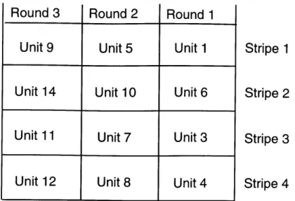
The need for synchronization arises due to the combination of two network effects: skew and striping unit loss. Due to skew, units on some stripes may arrive much later than expected. This would not be a problem if it were guaranteed that they would arrive eventually; the receiver could simply wait for striping units on stripes with longer delays to arrive before proceeding with the reassembly of the incoming data. However, the possibility that striping units may be lost complicates matters. In figure 2-5, striping unit 2 has been lost in the middle of transmission. Instead of the receiver correctly placing the units in sequential order, the order will be 1, 6, 3, 4, 5, etc.

If one of the striping units at the end of the data burst is lost, the receiver may be stuck

4

This calculation becomes more complex as different ports on the switch may have different line rates; the striping units we are examining will have to wait not only for traffic following the same path, but also for cross-traffic.

outgoing line rate4 . Multiplying the maximum queue difference times this time results in the maximum skew introduced due to queueing delay.

In order to convert the measure of skew in seconds to a measure of striping unit times, we calculate the length of a single striping unit time by dividing the length of a striping unit by the line rate into the destination host. By dividing the amount of skew time by this length, we get the amount of skew measured in striping unit times. For example, the length of an ATM cell time on an OC-3c link is 424 bits -- 155 Mbps, which is 2.73pus.

The fixed skew components should be relatively simple to protect against; once they have been determined, the parameters of the synchronization method can adjusted to com-pensate. However, the variable components may vary too widely for the synchronization method to efficiently protect against them. The best approach in some cases may be to set some maximum amount of skew for which the synchronization method will compensate and to treat any data skewed by more than that amount as loss. For example, consider two paths which have an average skew of 7.5 ms, but whose maximum skew may be as great as a second. The receiving host may set some limit on the skew that it will attempt to compensate for. This value may depend on timeouts in the network software; if an entire packet hasn't arrived in some amount of time, the software may consider it lost anyway, so there is no need to worry about skew larger than that amount of time.

(25)

Unit 9

Unit 5

Unit 1

Unit

14 Unit

10 Unit

6 Unit

11 Unit 7

Unit

3 Unit

12 Unit 8

Unit

4 Stripe 1

Stripe 2

Stripe 3

Stripe 4

Figure 2-5: Improper Reassembly Due to a Lost Striping Unit

waiting for data which will never arrive. In either of these cases, we have to rely on a higher layer protocol to either catch the erroneously reconstructed data units or to time out and signal the striping recovery algorithm that something is broken.

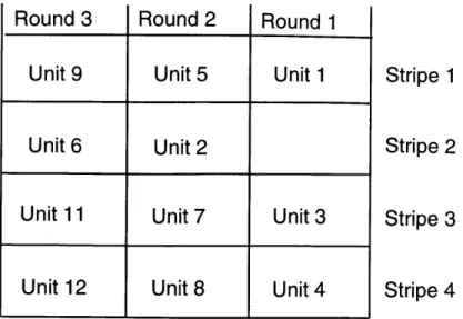
The algorithm just described compensates for skew but, as we have seen, offers no protection against lost striping units. The other obvious simple choice is to design the algorithm so that it detects lost striping units and ignores the possibility of skew. Assume again that the receiver is expecting striping units to arrive in a round robin order. When a striping unit arrives on a stripe, the receiver then goes to the next stripe and waits for a striping unit to arrive on that stripe. Since the receiver is not aware of the possibility of skew, if a striping unit arrives on the next stripe in the round robin order before one arrives on the current stripe in the order, the receiver believes that it has lost a cell.

This is illustrated in figure 2-6. The second stripe has enough additional delay such that striping units arrive one round later than they would if there were no skew. In this case, the receiver takes unit 1 from the first stripe and then moves to the second stripe. Since unit 3 arrives before unit 2, the receiver assumes that unit 2 was lost because it believes that the only order in which the units can arrive if they are not lost is 1, 2, 3, etc. However, since unit 2 arrives during the next round, it will be mistaken for the striping unit which really belongs in that round. Thus, the receiver will place the striping units in the order 1, 3, 4, 5, 2, 7, etc, which is clearly incorrect.

Obviously, in either case, something extra needs to be done to compensate for skew and

W

Round 1

Round 2

(26)

Unit 9

Unit 5

Unit 1

Unit 6

Unit 2

Unit

11 Unit 7

Unit

3 Unit

12 Unit 8

Unit

4 Stripe 1

Stripe 2

Stripe 3

Stripe 4

Figure 2-6: Improper Reassembly Due to Skew

data loss to allow the data arriving at the destination to be reconstructed in the proper order. In the next chapter, we will examine some well-known techniques for maintaining synchronization on a single channel and show how these can be applied to maintaining synchronization across a number of stripes.

2.5 Summary

Striping topology, host participation, and striping layer define the situation and architec-ture, and synchronization are the primary degrees of freedom associated with the imple-mentation. The remaining tools which we are missing are those concerned with the various options for implementing synchronization.

The largest problem associated with striping is that data loss and skew cause data to arrive at the destination misordered, something which does not occur when using a single channel. In the next chapter, we will examine some well-known techniques for dealing with synchronization on a single channel and show how these apply to striped channels.

The next chapter will also present some previous work related to network striping. These examples will demonstrate some of the validity of our reference model. In addition, they will present some examples of synchronization across multiple channels. Finally, they represent the exploration of the striping space which has already been performed; when determining the striping cases which we wish to investigate we will be able to set these aside.

(27)

Chapter 3 Previous Work

This chapter presents several flavors of previous work related to the striping problem. Recall from the previous chapter that the fundamental problem with striping data across multiple channels is maintaining or recovering the proper data order; the solution to this problem is to use some form of synchronization across the stripes. The first portion of previous work will examine the known techniques for synchronization on a single channel; we will find that similar approaches will apply to the multiple channel synchronization problem as well.

We will also examine several existing striping implementations, related to both networks and to disks. The discussion will be divided into ATM-related striping, ISDN striping, HiPPi striping, and disk striping. This work will present a good test of the framework developed in the previous chapter, as well as providing some examples of specific synchronization schemes.

3.1 Single Channel Synchronization

When transmitting data through a digital channel, there are several requirements beyond the physical equipment which provides the channel. Simply transmitting bits of data down the channel does not provide any way for the receiver to know when and where to start expecting data. Some means is necessary to allow the receiver to find the boundaries of bursts of data from the random bit stream it is receiving. To accomplish this, the transmitter encapsulates any data which it transmits in some form of frame; the receiver knows how to find the frames, which allows it to extract the higher layer data from the channel. In addition to framing, the receiver requires some way of determining if data has been lost

(28)

during transmission.

3.1.1 Framing

The process of framing involves surrounding the data with some recognizable pattern at the transmitter. This pattern is then used by the receiver to correctly recover the framed data. There are two basic ways to place the framing pattern into the data stream; patterns can either be placed at periodic or aperiodic intervals. Some combination of these two methods can be used as well.

Periodic Framing Patterns

This technique places an easily recognized pattern at periodic locations in the data stream at the transmitter. Initially, the receiver searches the incoming data for this pattern. Once it has found it, the receiver considers itself synchronized and then continuously verifies that the pattern reappears at the proper times. If the pattern does not appear, the receiver has lost synchronization and must return to the state where it is hunting for the pattern. A good example of an existing system which uses a periodic framing pattern is SONET[8].

The beginning of a basic SONET frame is marked by two bytes which are used by the transmission equipment to align to the start of a frame.

Aperiodic Framing Patterns

This technique is virtually identical to the one above, except that the pattern for which the receiver is searching can appear at random points in the data stream. This means that the receiver must always be searching for it. Many asynchronous data link control layers, such as HDLC[9], use an aperiodic framing pattern in the form of a flag which marks the end of a link idle period.

Spoofing

One problem with inserting a pattern which needs to be recognized by the receiver into the data which needs to be processed and forwarded by the receiver is the possibility that the real data will contain the framing pattern. This phenomena is known as spoofing. There are several techniques which are used to avoid spoofing. One method, used by SONET, is scrambling; the actual data is subjected to a transformation before being placed into the

(29)

SONET frames which reduces the probability that the data bytes will contain the start

of frame byte. Another method, used by HDLC, is bit-stuffing. In this case, the flag which marks the beginning of a frame contains a large number of consecutive ones; zeros are inserted into the data to prevent the same number of consecutive ones from appearing anywhere but the flag.

Yet another scheme for avoiding spoofing is coding. These schemes use a code to map a fixed number of bits of real data into a word with a larger number of bits which is then transmitted. The receiver performs the inverse mapping. Since the words which are transmitted contain more bits than the data words which are mapped into them, there will be some words left over which are reserved for the link protocol. These reserved words can be used to fill the transmission channel when the link is idle and to frame the real data so that it can be properly recovered1. The Hewlett-Packard G-Link chipset is an example of a transmission system which uses a coding scheme; it allows either 16B or 17B/20B or 20B or 21B/24B[1O].

3.1.2 Loss Detection

Another important requirement for transmission on a single channel is the ability to detect the loss of data elements. Again, there are several well-known schemes to accomplish this. One possible way is to attach some sort of a tag to each data element. Using the tags, the receiver can detect missing data. Sequence numbering is one simple example of a tagging scheme. Another method is to calculate the length of the frames being transmitted to the receiver and then to convey the length to the receiver. This is the method used to detect missing cells in AAL5 frames.

Note that a desirable aspect of a framing scheme is to convert framing errors into data losses. This will prevent incorrectly constructed frames from being passed up to the next layer as valid data.

3.1.3 Synchronization Methods Applied to Striping

We stated earlier that the primary difficulty with implementing striping is the possibility that the combination of skew and data loss will cause data to arrive at the destination

1In _{addition, the mapping into code words is arranged so that approximately the same number of ones}

(30)

Round 6 Round 5 Round 4 Round 3 Round 2 Round 1

Unit 5 Unit 1 Unit 13 Unit 9 Unit 5 Unit 1 Stripe 1

Unit 14 Unit 10 Unit 6 Unit 2 Stripe 2

Unit 3 Unit 15 Unit 11 Unit 7 Unit 3 Stripe 3

Unit 8 Unit 4 Unit 16 Unit 12 Unit 8 Unit 4 Stripe 4

Figure 3-1: Tagging Striping Units Across the Stripes

misordered. In order to prevent or compensate for this, some method of synchronization and data loss protection across the stripes are necessary. The standard tools for single channel synchronization can be applied here in order to accomplish this.

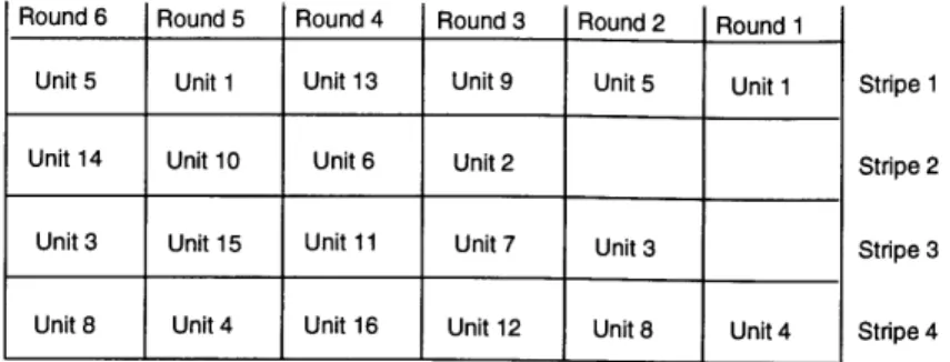
The first general approach that can be used is the tagging method applied to striping units across all the stripes (Figure 3-1). The first striping unit on the first stripe would get the first tag, the first unit on the second stripe would get the second, etc. This provides the destination with an absolute ordering scheme which it can use to determine not only the proper order of the incoming striping units but whether any units are lost as well. The largest drawback is that the cost in bits per striping unit increases rapidly as both the number of stripes and the amount of skew which must be protected against increases.

Another approach is to use the tagging method on a per stripe basis; the striping units on each stripe can then be tagged with the same set of tags (Figure 3-2). Data loss on each stripe is detected, and if there are n stripes, this scheme requires either 1/nth of the number of tags of the previous scheme or provides protection against n times more skew. The problem then becomes aligning the stripes so that the receiver performs its round robin rotation on units from the same transmitted round on each stripe. This has a simple solution, however, if we ensure that units from the same round at the transmitter get the same tag. The tag then becomes not only a sequence number on each stripe, it also becomes an indicator of the round number. The receiver can align each stripe on the same round number and be assured that, as long as the number of tags is long enough to protect against the skew introduced by the network, it will correctly reconstruct the original data. In a sense, the round numbers make up a type of frame on each stripe; the start of frame pattern is the first tag, and the length is the number of tags on each stripe.

Finally, there is the framing approach which is completely divorced from per-element

(31)

-~ I

~-Round 6 Round 5 Round 4 Round 3 Round 2 Round 1

Unit 2 Unit 1 Unit 4 Unit 3 Unit 2 Unit 1

Unit 4 Unit 3 Unit 2 Unit 1

Unit 1 Unit 4 Unit 3 Unit 2 Unit 1

Unit 2 Unit 1 Unit 4 Unit 3 Unit 2 Unit 1

Figure 3-2: Tagging Striping Units on Individual

Round 6 Round 5 Round 4 Round 3 1 Round 2 1 Round 1

S Stripe 1 Stripe 2 Stripe 3 Stripe 4 tripes Stripe 1 Stripe 2 Stripe 3 Stripe 4

Figure 3-3: Using Striping Elements with Metaframing Patterns

tagging. We will refer to this as metaframing. The transmitter places a well-known pattern in a striping element on each stripe at either periodic or random intervals (Figure 3-3). The receiver looks for this pattern and uses it to align the stripes so that it receives striping units from the same transmitter round during each receiving round. Failure to detect the pattern on one of the stripes means that the receiver has lost synchronization. This method provides synchronization and data loss protection reasonably cheaply in terms of the number of bits used. Protection against larger amounts of skew can be achieved by increasing the length of time between synchronization patterns. However, there is a cost in the lack of granularity in loss detection; the receiver can know that it has lost data in a frame but not necessarily which striping element in a frame was lost. There is also a cost in wasted time and network resources. A longer frame length will require more time before loss of synchronization can be detected; all of the striping units in a frame that has lost a striping unit may need to be dropped.

Of course, the metaframing and tagging approaches can be combined; the per stripe

tagging scheme can be viewed as metaframing with a metaframe size of one element, and a tag which indicates the location of the metaframe in a larger framing entity. To provide more protection against skew, either the length of the tags or the length of the metaframes

Data Framing Data Data Data Framing

Unit Unit Unit Unit Unit Unit

Data Data Data Framing

Unit Unit Unit Unit

Framing Data Data Data Framing

Unit Unit Unit Unit Unit

Data Framing Data Data Data Framing

(32)

could be increased, depending on what is required.

When we analyze possible striping cases in later chapters, we will only address the general tagging and framing synchronization possibilities, with the awareness that the com-binations can be generated in a straight-forward manner.

3.2 ATM Network Striping

We will examine two pieces of work which are concerned with striping related to ATM networks. The first is the Unison testbed ramp. The Unison testbed was one of the first efforts to build and study a network based on ATM[11]. Built prior to the standardization of the ATM cell, the Unison ATM cells consisted of 32 bytes of payload and 6 bytes of header and trailer combined. The testbed itself consisted of Cambridge Fast Rings (CFR) located at four sites; the sites were linked by European primary rate ISDN2_{. The Unison}

ramps were developed to connect the CFR at each site to the ISDN network. Each CFR operated at 50 Mbps, so the ramps striped data over the ISDN network in order to provide communication links of reasonable bandwidth, referred to as U-channels, between the sites. The second piece of work related to ATM striping the the Osiris host interface. Osiris is an ATM-based host interface for the DEC Turbochannel[12]. It was developed at Bellcore as part of the Aurora gigabit testbed[13]. It is connected to the Aurora SONET facilities at the OC-12 rate, and accomplishes this by generating four STS-3c signals which are placed into SONET frames and multiplexed into an OC-12 by a separate multiplexing board.

3.2.1 Unison

Each site in the Unison testbed had a number of local client networks. A single CFR at each site was used to interconnect these networks using ATM. In addition, each CFR was connected to a Unison ramp, which was in turn connected to the ISDN network. In order for hosts to communicate with hosts on other local networks, a local network management facility would maintain ATM connections between the two networks through the CFR, and a higher layer protocol would use these ATM connections as part of the path between the hosts. In order to communicate with hosts at other sites, a local ATM connection would

2

ISDN in Europe provides 30 64 kbps B-channels for data and 2 64 kbps D-channels for signalling, as