HIV/AIDS and Development: A Reappraisal of the Productivity and Factor Accumulation Effects

(1)

Productivity and Factor Accumulation Eﬀects

Online Appendix

By Th´eophile T. Azomahou, Raouf Boucekkine, and Bity Diene∗

I. Further Details on Data: Variables and Sources

This section provides further details on data. It includes the main economic and demographic indicators of the model and their source.

- Economically active population, by age and sex (1980-2020). The data come from the International Labor Organization. The database contains world, regional and country estimates and projections of the total population, the activity rates and the economically active population (labor force) by sex and five-year age groups (from 10 to 64 years and 65 years and over).

- HIV-seroprevalence (1980-2015). The data is provided by the US Census Bureau, International Programs Center.

Estimated HIV adult prevalence trends from 1980 to 2015. These estimates were derived from the Epidemic Projection Package, an epidemiologically sound computer model that allows for a “best fit” of HIV prevalence data from antenatal clinic women who come in for their first antenatal visit. HIV prevalence is defined as the percentage of women surveyed testing positive for HIV. Each year a national survey of HIV prevalence among women at-tending public antenatal clinics in South Africa is conducted by the Depart-ment of Health. The Annual HIV antenatal survey provides South Africa with annual HIV trends among pregnant women and further provides the basis for making other estimates and projections on HIV/AIDS trends.

∗ _{Azomahou: United Nations University (UNU-MERIT), Maastricht University, University of}

Au-vergne and CERDI, Tel: +31 433 884 440, Fax: +31 433 884 499 (azomahou@merit.unu.edu). Boucekkine: Aix-Marseille University (AMSE), CNRS and EHESS, (raouf.boucekkine@univ-amu.fr). Diene: University of Auvergne and CERDI, (bity.diene@udamail.fr). We would like to thank Matteo Cervellati, Miguel Perez-Nievas, Noel Bonneuil, Frédéric Dufourt, Frédéric Docquier and Vladimir Ve-liov for helpful comments. Insightful discussions with Elizabeth Asiedu are gratefully acknowledged. This work was supported by the FERDI (Fondation pour les Etudes et Recherches sur le Développement International) and the Agence Nationale de la Recherche of the French government through the program “Investissements d’avenir ANR-10-LABX-14-01.”

(2)

- HIV+ (1990-2015). This indicator is defined as the number of people

in-fected. The Demographic impact of HIV/AIDS in South Africa follows from National Indicators for 2004.

- Life expectancy at birth by sex (1920-2015). The data are part of the World Development Indicators, Health Nutrition and Population, and partly pro-vided by the League of Nations, Northwestern University. This is the num-ber of years that a new-born could live if the normal conditions of mortality at birth were the same ones throughout life.

- Total health expenditure (1960-2000). The data are extracted from the Health Nutrition and Population database.

- Percentage expenditure of AIDS in total health expenditure (1960-2000). The data are extracted from South African Budget Review, 2003/04 and the Estimates of the National Expenditure, 2003.

- Unemployed by age and sex (2000-2003). The data come from the Interna-tional Labor Organization.

The series on unemployment shown here relates in principle to the entire ge-ographical area of a country. In 1982, the Thirteenth International Confer-ence of Labor Statisticians adopted a new Resolution concerning Statistics of the Economically Active Population, Employment, Unemployment and Underemployment, in which the definition of unemployment is revised. The new definition is to a large extent similar to the earlier definition adopted by the Eighth Conference. However, it introduces some amplifications and modifications concerning, in particular, the criteria of seeking work and cur-rent availability for work, the statistical treatment of persons temporarily laid oﬀ, persons currently available for work but not actively seeking work, etc. The changes are aimed to make it possible to measure unemployment more accurately and more meaningfully in both developed and developing countries.

- GDP per capita (1960-2000). The data come from Penn World Table 6.1.

- Saving rates with and without AIDS. We use data fromFreire (2004).

II. Recent findings on the Ben-Porath Mechanism

The introduction of the Ben-Porath mechanism is a strong point of our contri-bution. This mechanism has recently sparked a strong debate in the literature. Following the seminal contribution of Ben-Porath (1967), the idea emerged that the gains in life expectancy positively impact schooling by increasing the hori-zon over which investments in schooling have been paid oﬀ. The rational of the

(3)

to the future rewards that this human capital will receive. Several prominent pre-dictions have been based on this mechanism, including the fact that an increase in rental rate on human capital will increase future rewards to human capital and as a result, increase investment in schooling.

Hazan (2009) challenged this view by claiming that an increase in expected

lifetime labor supply is a necessary condition for an increase in longevity to induce more investment in schooling. Hazan (2009) then presents evidence of a sharp reduction in expected total working hours for US workers born in the period 1840-1970 that the author interprets as pointing to a violation of the necessary condition and concludes that the reduction in mortality rates in the U.S. over this period cannot account for any of the increase in education attainment. This conclusion has very important policy implications since it challenges the view that reducing mortality and improving health conditions may promote the acquisition of human capital, since it questions the empirical rationale of studying the relation between mortality and human capital.

Recently, Cervellati and Sunde(2013) pointed that the model inHazan(2009) assumes a perfectly rectangular survival probability and a linear human capi-tal production function, meaning that individuals are assumed to survive with probability one during all their life, and die with probability one when reach-ing their life expectancy. As result, mortality can aﬀect the education decision only by extending the maximum longevity, but not by changing the probability of surviving during working ages. The assumption inHazan(2009) is a strong coun-terfactual and hides the eﬀect of observed changes in age-specific mortality rates on the costs and benefits of education which is presents most theoretical frame-works that study endogenous schooling in the context of changing mortality, e.g.

de la Croix and Licandro (1999), Boucekkine, de la Croix and Licandro (2002),

Boucekkine, de la Croix and Licandro(2003),Soares(2005),Cervellati and Sunde

(2005).1

Cervellati and Sunde (2013) generalized the framework of Hazan (2009) and

showed that, the necessary condition for a reduction in mortality rates to induce more years of schooling is that the increase in longevity is related to an increase in the benefits of schooling relative to the opportunity costs of a delayed entry into the labor market. The authors also replicate the empirical analysis ofHazan

(2009), and found no evidence that greater longevity has been associated with a decline in the relative benefits of schooling. This debate highlights the fact that the Ben-Porath mechanism is still valid in explaining the data.

III. Further Methodology

In this section, we present the forecasting methodology and the projection of HIV prevalence. The forecasting first needed the estimation of the parameters

1_{In a theoretical setting,}_{Boucekkine, Diene and Azomahou}₍₂₀₀₈_{) considered physical capital}

accu-mulation, schooling, health expenditures and supply eﬀects within aBlanchard(1985) two-sector economy to capture life-cycle eﬀects of AIDS-like epidemics.

(4)

of an assumed econometric specification underlying the data generating process. For this purpose, we retain a Gaussian ARM A(p, q) process for which we describe below the estimation and the forecasting procedure.2 Further details on these statistical methods can be found inHamilton(1994).

A. Estimation

A Gaussian ARM A(p, q) process is described as:

Yt= α + ϕ1Yt−1+ ϕ2Yt−2+· · · + ϕpYt−p+ ut

+ θ1ut−1+ θ2ut−2+· · · + θqut−q t = 1,· · · , T

(1)

where ut ∼ i.i.d N(0, σ2), and where the vector of population parameters θ =

(α, ϕ1, ϕ2,· · · , ϕp, θ1,

θ2,· · · , θq, σ2)′ is to be estimated. The approximation to the likelihood function

is conditioned on both initial values of the y′s and u′s. Assuming that the initial

values for y0 ≡ (y0, y−1,· · · , y−p+1)′ and u0 ≡ (u0, u−1,· · · , u−p+1)′ are given, the sequence{u1, u2,· · · , uT} can be computed from {y1, y2,· · · , yT} by iterating

on

ut= yt − α − ϕ1yt−1− ϕ2yt−2− · · · − ϕpyt−p

− θ1ut−1− θ2ut−2− · · · − θqut−q t = 1,· · · , T

(2)

The conditional log likelihood is given by:

L(θ) = ln fYT,YT−1,··· ,Y1|Y0,u0(yT, yT−1,· · · , y1|y0, u0; θ) = −T 2 ln(2π)− T 2 ln(σ 2₎₋ T ∑ t=1 u2_t 2σ2 (3)

In maximizing this log likelihood, we set the initial y′s and u′s to their expected

values. That is ys = α/(1− ϕ1− ϕ2− · · · − ϕp) for s = 0,−1, · · · , −p + 1, and

us= 0 for s = 0,−1, · · · , −p + 1. Then, we proceed with the iteration in (2) for

t = 1,· · · , T . We estimate a multiple ARMA(p, q) model with p = 2 and q = 2,

which turns out to be an estimate of six models. We finally select the model that optimizes the Schwarz Criterion. The selected model is used for forecasting.

2_{Prior to using the ARMA process, we considered a more flexible forecasting AFRIMA (Fractional}

Integrated ARMA) framework: AF RIM A(p, d, q), where d is the degree of integration. Indeed, while it roved to be a good alternative forecasting method, the ARMA approach has an inherent weakness in falling to distinguish between unit root non-stationarity and ‘gradual’ non-stationarity (i.e., between stationary and unit root). Estimation results based on data at hand show that d≃ 0, which turns out to be a typical ARMA process.

(5)

B. Forecasting

Now, consider forecasting the stationary and invertible ARM A(p, q):

(4) (1− ϕ1L− ϕ2L2− · · · − ϕpLp)(Yt− µ) = (1 + θ1L + θ2L2+· · · + θqLq)ut

where L is the lag operator and µ is the unconditional mean E(Yt). The

one-period-ahead forecast (s = 1) is given by:

( ˆY_t+1_|t− µ) = ϕ1 (Yt− µ) + ϕ2(Yt−1− µ) + · · ·

+ ϕp(Yt−p+1− µ) + θ1uˆt+ θ2uˆt−1+· · · + θquˆt−q+1

(5)

with ˆu generated recursively from ˆu = Yt− ˆYt|t−1. Finally the s-period-ahead

forecasts based on the Wiener-Kolmogorov prediction formula are:

C. Projection of HIV Prevalence

To obtain the projected HIV prevalence, we fit a double logistic curve of the form (6) p(t) = [ eα(t−τ) 1 + eα(t−τ) ] [ ae−β(t−τ) 1 + eβ(t−τ) + b ]

where α is the rate of increase at the start of the epidemic, a denotes the peak value, β is the rate of convergence, b is the final prevalence level and τ shifts the whole curve backward. The value of α is chosen so that the doubling time is 1.5 years. The latter is chosen so that the doubling time at the beginning of the epidemic can be ln(2)/α. This means that α = ln(2)/1.5. As a result, for a given β, we have to find (numerically) the parameters a, b and τ solution of the nonlinear system: S (a, b, τ) =          p(0) = 0.1916 = _1+ee−ατ_−ατ [ aeβτ 1+eβτ + b ] p(2015) = 0.194 = _1+eeα(15_α(15−τ)−τ) [ ae−β(15−τ) 1+e−β(15−τ) + b ] ˙ p(t) = 0⇐⇒ α eα(t−τ) [ ae−β(t−τ) 1+e−β(t−τ) + b ] = aβe−β(t−τ) [1+e−β(t−τ)]2 with t = 3.

(6)

where ˙p(t) = dp(t)_dt . The first equation of the system corresponds to the starting period (t = 0 for year 2000 where the prevalence is 0.1916), the second denotes the ending period (t = 16 for year 2015 where the prevalence is 0.194) and the third equation expresses the peak of the epidemic. The value t = 3 represents the diﬀerence between the peak year 2003 and the starting date 2000.

IV. Additional Results

A. Prevalence

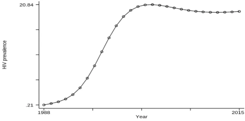
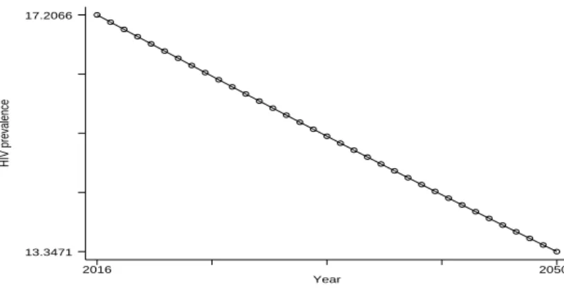
Figure 1 plots the HIV prevalence rate from 1980 to 2015 as constructed by the US Census Bureau. In order to obtain HIV prevalence projections, we first solve numerically the nonlinear system given by S (a, b, τ) for a, b and τ. We obtain a = 0.4045, b = 0.0003 and τ =−9.356. These values are then plugged into relation (6) to determine HIV prevalence from 2016 to 2050. The result is provided in Figure2. The scenario studied is therefore a continuous (but not very fast) decrease in this rate after 2015, which seems reasonable.

HIV prevalence

Year

1988 2015

.21 20.84

Figure 1. – HIV prevalence in percent, 1988-2015

B. Saving

Figure 3 displays our forecast (both the median forecast and the density esti-mate of the forecasted values) of saving without and with AIDS. The forecasts are stable over time, after 2020. The confidence intervals are excellent for both. We shall notably observe here that the gap in saving rates between the AIDS and non-AIDS cases does not deepen dramatically after 2020. It is about 2 percent in 2015 and it is on average around 3 percent after 2020.

(7)

HIV prevalence

Year

2016 2050

13.3471 17.2066

Figure 2. – HIV prevalence, 2016-2050

C. The Economic Growth of HIV/AIDS Quantified

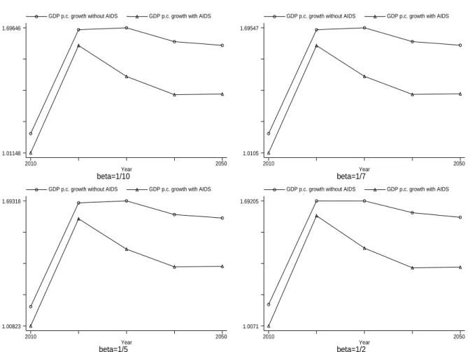
The sharp trends in mortality and life expectancy induced by AIDS will def-initely be more pronounced after 2020. These demographic paths are likely to induce a delayed eﬀect of AIDS on economic growth, the main channels being the size of the active population in the medium run (say between 2020 and 2040), and the Ben-Porath eﬀect via the productivity specification at least when parameter

β is large enough.

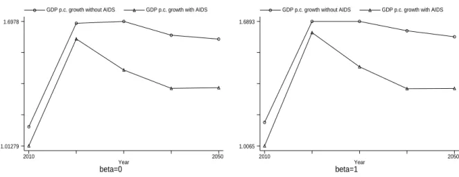
Actually the delayed eﬀect turns out to be strong in all our simulations, as transpires from Figures 4 and 5 for growth per capita when β varies from 0 to 1.3 Whatever the value of β, the gap between the AIDS and no-AIDS scenarios is rather stable between 2010 and 2020, but then it increases sharply between 2020 and 2030. The gap keeps increasing but at an apparently much lower pace between 2030 and 2040. Finally, the gap seems to be stable (or shrinks very slightly) after 2040, featuring a kind of long-run economic growth eﬀect of AIDS.

3_{The growth rates reported in the figures are “cumulative” growth rates over the successive decades.}

In order to get an average annual growth rate over a given decade, one has to divide the associated growth rate registered during the decade by 10.

(8)

16 18 20 22 24 26 28 30 32 34 2000 2010 2020 2030 2040 2050 2060 Actual save Median Forecasts 95% Confidence Bands 0 0.5 1 1.5 2 2.5 29.6 29.8 30 30.2 30.4 30.6 30.8 31 31.2 31.4 31.6 saveForecast Kernel Density for Observation 2015

N(s=0.33) 19 20 21 22 23 24 25 26 27 28 29 1990 2000 2010 2020 2030 2040 Actual savew Median Forecasts 95% Confidence Bands 0 0.2 0.4 0.6 0.8 1 1.2 1.4 1.6 1.8 2 26.4 26.6 26.8 27 27.2 27.4 27.6 27.8 28 28.2 28.4 28.6 savewForecast Kernel Density for Observation 1999

N(s=0.355)

(9)

beta=1/10

Year

GDP p.c. growth without AIDS GDP p.c. growth with AIDS

2010 2050

1.01148 1.69646

beta=1/7

Year

2010 2050

1.0105 1.69547

beta=1/5Year

2010 2050

1.00823 1.69318

beta=1/2Year

2010 2050

1.0071 1.69205

(10)

beta=0

Year

2010 2050

1.01279 1.6978

beta=1

Year

2010 2050

1.0065 1.6893

(11)

D. Robustness: Sensitivity Results for β = 0, 1₇, 1₅, 1₂ and 1

Table 1— – Growth rates (in percentage) of GDP per capita: gap between the AIDS and no-AIDS

scenarios for varying the health productivity parameter ζ for β = 1

ζ 1 2.5 5 10

Year GDP per cap GDP per cap GDP per cap GDP per cap

2010 0.86 0.86 0.87 0.89

2020 0.89 0.89 0.89 0.89

2030 2.78 2.78 2.78 2.78

2040 3.18 3.18 3.18 3.18

2050 2.84 2.84 2.84 2.84

Table 2— – Growth rates (percentage) of GDP per capita: gap between the AIDS and no-AIDS

scenarios for varying the health productivity parameter ζ for β = 1/2

ζ 1 2.5 5 10

2010 0.85 0.85 0.86 0.89

2020 0.88 0.88 0.88 0.88

2030 2.72 2.72 2.72 2.72

2040 3.02 3.02 3.02 3.02

2050 2.74 2.74 2.74 2.74

Table 3— – Growth rates (percentage) of GDP per capita: gap between the AIDS and no-AIDS

ζ 1 2.5 5 10

2010 0.84 0.84 0.85 0.89

2020 0.87 0.87 0.87 0.87

2030 2.68 2.69 2.68 2.68

2040 2.93 2.93 2.93 2.93

(12)

ζ 1 2.5 5 10

2010 0.84 0.84 0.85 0.88

2020 0.86 0.86 0.86 0.86

2030 2.68 2.67 2.68 2.67

2040 2.91 2.92 2.92 2.90

2050 2.68 2.68 2.67 2.67

ζ 1 2.5 5 10

2010 0.83 0.84 0.85 0.88

2020 0.86 0.86 0.86 0.86

2030 2.67 2.67 2.67 2.66

2040 2.90 2.90 2.90 2.90

2050 2.67 2.67 2.67 2.66

scenarios for varying the health productivity parameter ζ for β = 0

ζ 1 2.5 5 10

2010 0.83 0.84 0.85 0.87

2020 0.86 0.86 0.86 0.86

2030 2.65 2.65 2.65 2.65

2040 2.87 2.87 2.87 2.87

(13)

REFERENCES

Ben-Porath, Yoram. 1967. “The production of human capital and the life cycle of earnings.” The Journal of Political Economy, 352–365.

Blanchard, Olivier. 1985. “Debt, deficits, and finite horizons.” Journal of

Po-litical Economy, 93: 223–47.

Boucekkine, Raouf, Bity Diene, and Th´eophile T. Azomahou. 2008.

“Growth economics of epidemics: A review of the theory.” Mathematical

Pop-ulation Studies, 15: 1–26.

Boucekkine, Raouf, David de la Croix, and Omar Licandro. 2002. “Vin-tage human capital, demographic trends, and endogenous growth.” Journal of

Economic Theory, 104(2): 340–375.

Boucekkine, Raouf, David de la Croix, and Omar Licandro. 2003. “Early mortality declines at the dawn of modern growth.” Scandinavian Journal of

Economics, 105: 401–418.

Cervellati, Matteo, and Uwe Sunde. 2005. “Human capital, life expectancy, and the process of development.” The American Economic Review, 95: 1653– 1672.

Cervellati, Matteo, and Uwe Sunde. 2013. “Life expectancy, schooling, and lifetime labor supply: Theory and evidence revisited.” Econometrica, 81: 2055– 2086.

de la Croix, David, and Omar Licandro. 1999. “Life expectancy and en-dogenous growth.” Economics Letters, 65: 255–263.

Freire, Sandra. 2004. “Impact of HIV/AIDS on saving behaviour in South Africa.” TIPS/DPRU/Cornell University Forum: African Development and Poverty Reduction.

Hamilton, James Douglas. 1994. Time Series Analysis. Vol. 2, Princeton Uni-versity Press.

Hazan, Moshe. 2009. “Longevity and lifetime labour supply: Evidence and implications.” Econometrica, 77: 1829–1863.

Soares, Rodrigo R. 2005. “Mortality reductions, educational attainment, and fertility choice.” The American Economic Review, 95: 580–601.