Publisher’s version / Version de l'éditeur:
Questions? Contact the NRC Publications Archive team at
PublicationsArchive-ArchivesPublications@nrc-cnrc.gc.ca. If you wish to email the authors directly, please see the
https://publications-cnrc.canada.ca/fra/droits
L’accès à ce site Web et l’utilisation de son contenu sont assujettis aux conditions présentées dans le site LISEZ CES CONDITIONS ATTENTIVEMENT AVANT D’UTILISER CE SITE WEB.
Student Report; no. SR-2009-17, 2009-01-01
READ THESE TERMS AND CONDITIONS CAREFULLY BEFORE USING THIS WEBSITE.
https://nrc-publications.canada.ca/eng/copyright
NRC Publications Archive Record / Notice des Archives des publications du CNRC :
https://nrc-publications.canada.ca/eng/view/object/?id=ef6c81c8-89cc-40ec-9895-1aa2486a7e83 https://publications-cnrc.canada.ca/fra/voir/objet/?id=ef6c81c8-89cc-40ec-9895-1aa2486a7e83
NRC Publications Archive
Archives des publications du CNRC
For the publisher’s version, please access the DOI link below./ Pour consulter la version de l’éditeur, utilisez le lien DOI ci-dessous.
https://doi.org/10.4224/18253250
Access and use of this website and the material on it are subject to the Terms and Conditions set forth at Porting of the Wave Analysis Module to SWEET
National Research Council Canada Institute for Ocean Technology Conseil national de recherches Canada Institut des technologies oc ´eaniques
SR-2009-17
Student Report
Porting of the Wave Analysis Module to SWEET.
Young, A.
Young, A., 2009. Porting of the Wave Analysis Module to SWEET. St. John's, NL : NRC Institute for Ocean Technology. Student Report, SR-2009-17
DOCUMENTATION PAGE
REPORT NUMBER
SR-2009-17
NRC REPORT NUMBER DATE
August 2009
REPORT SECURITY CLASSIFICATION
Unclassified
DISTRIBUTION
Unlimited
TITLE
PORTING OF THE WAVE ANALYSIS MODULE TO SWEET AUTHOR(S)
Adam Young
CORPORATE AUTHOR(S)/PERFORMING AGENCY(S)
Institute for Ocean Technology, National Research Council, St. John’s, NL
PUBLICATION
SPONSORING AGENCY(S)
Institute for Ocean Technology, National Research Council, St. John’s, NL
IOT PROJECT NUMBER NRC FILE NUMBER
KEY WORDS
GEDAP, Wave Analysis, ZCA, VSD, SWEET
PAGES FIGS. 8 TABLES SUMMARY
This document serves as a reference to future developers working on or with the wave analysis modules in SWEET (ZCA, VSD, FFT). It provides background information on design decisions as well as an overview of the math involved in each module.
ADDRESS National Research Council
Institute for Ocean Technology Arctic Avenue, P. O. Box 12093 St. John's, NL A1B 3T5
National Research Council Conseil national de recherches Canada Canada
Institute for Ocean Institut des technologies Technology océaniques
Porting of the Wave Analysis Module to Sweet
SR-2009-17
Adam Young
Contents
1 Introduction………..1
2 Zero Crossing Analysis………2
2.1 Overview 3
2.2 Down Crossing Analysis 3
2.3 Pre-Analysis Processing 4
2.4 Wave Train Analysis 4
3 FFT Module……….7
4 VSD Module………....8
4.1 Design Overview 8
4.2 Wave Train Processing 8
4.3 Spectral Smoothing 9
4.4 Spectral Moment Calculation 11
1
1 Introduction
At the current time, the Software Engineering Group (SEG) of the National Research
Council’s (NRC) Institute for Ocean Technology (IOT) is switching to Python as its
preferred programming language. With some exceptions, the majority of new software
the department is producing is being written in Python. Older software already in use is
also being ported to the language. The reason for this transition to Python is beyond the
scope of this report. Instead, a closer look at the porting process of a specific module will
be performed. Development decisions and mathematical background of the module will
be explored providing future developers reference when attempting to update or interface
with the software.
The module in question is the Wave Analysis Module, which is part of the
Generalized Experiment Control and Data Acquisition Package (GEDAP). The GEDAP
software is written in Fortran and currently runs in a Virtual Memory System (VMS)
environment. To access the software, users usually connect to a VMS server remotely
through a command line terminal called GECKO. Transferring data to and from the
GEDAP software for analysis can become tedious as it involves running exportation
routines and sometimes editing files in excel.
This incompatibility of current Python software and GEDAP is the main reason
for porting the functionality of the Wave Analysis Module to the Software Environment
for Experimental Technologies (SWEET). SWEET is a Python framework developed by
IOT and the Institute for Information Technology (IIT) that provides groundwork for data
manipulation and analysis. By integrating functionality from the Wave Analysis Module
available in the framework. In particular, the Channel and ChannelCollection data
structures provide versatile methods of data storage with multiple built in math routines.
The Wave Analysis Module itself is actually made of multiple smaller modules.
These consist of a Zero Crossing Analysis (ZCA) module, a Fast Fourier Transform
(FFT) module and a Variance Spectral Density (VSD) module. Each of these is
implemented separately in SWEET. Although developed as stand alone tools, the ZCA
and VSD modules could easily be integrated as part of the Channel class as they both
take a channel object containing a wave train as their main argument. Despite this, the
fact that they both do not alter the original channel and produce a separate
3
2 Zero Crossing Analysis
2.1 Overview
The ZCA module is the simplest of the modules from a mathematical standpoint. The
analysis is performed completely in the time domain and does not involve calculus.
Although given a generalized name of zero crossing analysis, the module actually
performs a down crossing analysis in order to calculate basic wave train statistics such as
wave height and average period. The raw data from the down crossing analysis can be
used to calculate both down crossing and up crossing parameters.
2.2 Down Crossing Analysis
In a down crossing analysis a wave cycle is classified as shown in Figure 1. The
cycle starts with a zero crossing that precedes a trough and ends with the zero crossing
that follows the adjacent crest. This definition is important for the analysis as any part of
the wave train that appears before a full wave cycle is discarded. This discarded portion
is indicated in Figure 1 as the “Cut Off Region”.
2.3 Pre-Analysis Processing
Before any analysis is performed the wave train undergoes a trend removal
process. The type of trend removal is user specified upon calling the function. There are
options for removing a mean, removing a linear trend, and providing a mean to remove.
These options ensure that the time series is not shifted or skewed in a manner that will
hinder a zero crossing analysis.
In order for the analysis to be accurate it requires an average of fifty sample
points per wave. If this requirement is not met the wave train must be resampled. The
current implementation uses a cubic spline routine built into the Channel object of
SWEET. After isolated testing of the spline routine it has been proven to produce
identical results to routines provided by GEDAP.
2.4 Wave Train Analysis
Once the wave train is in an acceptable form the actual down crossing analysis
takes place. During the analysis troughs and crests are processed sequentially until the
last full trough or the last full crest is encountered. This means that an analysis may end
midway through a full wave cycle. For each cycle four points are recorded; the down
crossing time to start the wave, ordered pairs for the trough and crest, and the up crossing
time between trough and crest. Due to the data being discrete, it is almost certain that
points will not lie perfectly on zero crossings or maxima/minima, therefore interpolation
is used to calculate these points.
Crest and trough values are calculated using a parabolic fit of the highest/lowest
5
regression calls produced a bottleneck that slowed overall execution speed to an
unacceptable level. A simple math expression for the quadratic equation of a line passing
through three points was therefore derived to maximize speed. This is more criptic than a
named function call but is the only way to eliminate the bottleneck.
Calculation of zero a crossing time is more straightforward. First, the two sample
points that occur on either side of a zero crossing are found. Then, simple linear
interpolation is used to find the time at which the zero crossing occurs.
An important aspect of the ZCA is noise removal. This is accomplished in two
different ways. The first is a minimum wave threshold. This comes into effect during the
processing of the waves. To register a crest the wave train must not only produce
positive y-value samples, but also the samples must be larger than the minimum wave
threshold. No matter how many consecutive values appear above the x-axis, a crest will
not register until at least one point crosses the minimum wave threshold. This also
applies to troughs but the minimum wave threshold is inverted. Noise reduction is also
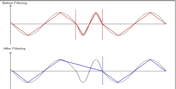
obtained through minimum period filtering. This is performed after the wave train has
been processed. Each wave is checked to ensure that its length is greater than the
minimum period. If it is not, the wave's zero crossings, trough point and crest point are
removed, absorbing it into the preceding wave. This is shown above in Figure 2 where
the middle wave cycle is shorter than the minimum period. After filtering it is absorbed
7
3 FFT Module
The fft module provides the low level functionality needed in a VSD analysis. It
was produced in SWEET as a stand-alone module in order to supply the rest of the
framework with access to fft routines. The actual fft calculations are performed by
SciPy's built in fft method. This pre-built function is paired with some data processing to
provide the exact functionality present in the GEDAP module. One of the most
prominent features is that data sets passed into the fft must have a length that is a power
of two. This was done for a few reasons. Firstly, it is specifically stated in the
documentation for SciPy's fft method that it is most efficient on data that has a length that
is a power of two. SciPy does offer an option for zero padding to this length in the fft
routine, however zero padding is not the only way. Other methods such as resampling
may be preferred. By forcing the data to already be of optimal length it ensures quick
execution time and leaves it up to the user to determine how they would like to alter the
data to meet the requirement. Secondly, requiring an optimal length matches the manner
in which the GEDAP implementation expects its arguments.
The form of the input argument for the inverse fft is in a fairly unusual form. It
takes a channel collection consisting of a real and an imaginary channel that represent a
spectrum to be transformed. This decision was made so that the output of the forward fft
routine could be used in its unaltered form with the inverse fft routine to produce the
4 VSD Module
4.1 Design Overview
The VSD analysis contains the most complicated math of the wave analysis
package. It is a lengthy process and is therefore divided into multiple functions. The
way in which it was divided was chosen to mimic the division of GEDAP’s VSD routine,
as focus during development was to obtain a working module. From a Pythonic
viewpoint, this was not the best way in which to separate the module. For purposes of
testing and clarity some of the larger functions such as spectral_density and
moving_average_filter should have been broken down further into smaller functions
based on different low-level functionality. Some processing in the vsd method should
have also been split into its own function to keep the main method, which will be used
externally, as clean as possible. Given time, a refactoring of this module would improve
clarity but is unnecessary for functionality.
4.2 Wave Train Pre-processing
Before a wave train is passed to the fft routine it undergoes some processing.
First, its length is converted to be a power of two. This ensures an efficient execution of
the fft. It can also improve leakage in the spectrum. The method for extending length
varies depending on the data. If the wave train is non-cyclic then it is zero padded until it
reaches an acceptable length. All zeros added are appended to the end of the data. In the
case of a cyclic wave train, re-sampling is used to preserve its cyclic nature.
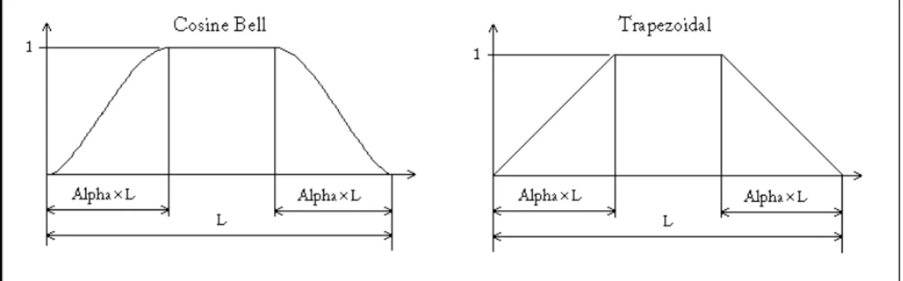
For non-cyclic data, a data window may also be applied. This is done after zero
9
an alpha value. Alpha represents the ratio of the length of the wave that is to be tapered.
Each end is tapered the same amount meaning alpha values must fall between 0.0 and
0.5. Examples of the data windows are shown in Figure 3 below.
4.3 Spectral Smoothing
After the Fourier transform smoothing of a spectrum is performed by a moving
average filter. Successive values in the spectrum are averaged together into fewer values
and the process acts as a low pass filter eliminating high frequency noise. Just how high
a frequency to eliminate is determined by the filter bandwidth or degrees of freedom the
user desires. Equation 1 relates the two values, where m is the length of the wave train
before zero padding / re-sampling, dt is the wave train sampling period just before the fft,
and alpha is the value used to specify data window size.
Figure 3: Data Window Types
The desired bandwidth is then used to determine the size of the averaging window
needed. This relationship is show in Equation 2 where n is the length of the wave train
after padding / re-sampling.
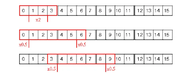
This window size dictates the number of values used in each averaging calculation as
well as the number of values in the filtered spectrum. Figure 4 shows the first three
iterations of a moving average filter with averaging window of three. It should be noted
that the averaging filter used for vsd is actually a moving sum filter. All numbers in the
averaging window are summed together but are not divided by the number of values in
the window. This still smoothes the spectrum but affects the scaling.
Equation 2: Averaging Window Size
11
4.4 Spectral Moment Calculation
Calculation of spectral moments is one of the most important parts of the vsd
module. Almost all other spectral attributes are determined using these moments.
Although based on a simple integral, these moments present a problem, as they have to
be calculated on very large data sets. To obtain the execution speed required, the integral
was derived to an algebraic expression representing the nth spectral moment of a straight
line between two points. This expression is then applied to each set of adjacent values in
the spectrum. The general formula for a kth order spectral moment is show in Equation 3.
Here f represents frequency and S(f) is the spectral value at f. Equation 4 shows the
integral derived for a straight line between two points, (X1, Y1) and (X2, Y2).
4.5 Formula Discrepancy
During the porting process an irregularity was found in the formula for Goda’s
Peakedness Factor. The expression programmed into GEDAP did not match the
expression found in reference material. The reference material was dated after
development of the module so the newer formula was used. This is the only value
Equation 3: Spectral Moment Integral
produced in SWEET’s vsd routine that will not match the corresponding value from